Analytical light curves in the realistic model for GRB afterglows

Abstract

Afterglow light curves are constructed analytically for realistic gamma-ray burst remnants decelerating in either a homogeneous interstellar medium or a stellar wind environment, taking into account the radiative loss of the blast wave, which affects the temporal behaviors significantly. Inverse Compton scattering, which plays an important role when the energy equipartition factor $\epsilon_{e}$ of electrons is much larger than that of the magnetic field ($\epsilon_{B}$), is considered. The inverse Compton effect prolongs the fast-cooling phase markedly, during which the relativistic shock is semi-radiative and the radiation efficiency is approximately constant, $\epsilon=\epsilon_{e}$. It is further shown that the shock is still semi-radiative for quite a long time after it transits into the slow-cooling phase, because of a slow decreasing rate of the radiation efficiency of electrons. The temporal decaying index of the X-ray afterglow light curve in this semi-radiative phase is $(3p-2+2\epsilon)/(4-\epsilon)$ in the interstellar medium case, and $[3p-2-(p-2)\epsilon]/2(2-\epsilon)$ in the stellar wind case, where $p$ is the distribution index of the shock-accelerated electrons. Taking $p=2.2$ — 2.3 as implied from common shock acceleration mechanism, and assuming $\epsilon_{e}\sim 1/3$, the temporal index is more consistent with the observed $\langle\alpha_{X}\rangle\sim 1.3$ than the commonly used adiabatic one. The observability of the inverse Compton component in soft X-ray afterglows is also investigated. To manifest as a bump or even dominant in the X-ray afterglows during the relativistic stage, it is required that the density should be larger than $\sim 1-10$ cm^-3 in the interstellar medium case, or the wind parameter $A_{\ast}$ should be larger than $\sim 1$ in the stellar wind case.

1 Introduction

In the past seven years, tremendous progress in understanding the cosmic gamma-ray bursts (GRBs) has been achieved from the detections of long-lived GRB embers (or afterglows) in low frequency bands (for reviews see van Paradijs, Kouveliotou, & Wijers 2000; Cheng & Lu 2001; Mészáros 2002; Zhang & Mészáros 2004; Piran 2004). The simple standard shock model (Mészáros & Rees 1997; Sari, Piran, & Narayan 1998) responsible for the afterglow has been successfully established (Wijers, Mészáros, & Rees 1997; Vietri 1997; Waxman 1997; Galama et al. 1998).

As more and more afterglows being detected, the energetics of GRB remnants and shock microphysics have been inferred within the context of the standard model. Although the standard model are in rough agreement with afterglow observations, problems still exist since the standard scenario is oversimplified at least in two aspects. First, in the standard afterglow model the relativistic shock is usually assumed to be quasi-adiabatic. However, the shock in fact may be partially radiative. Fittings to observed afterglows reveal that the shock imparts an equipartition amount of energy into electrons, which is responsible for both the afterglow emission and the shock energy loss (Panaitescu & Kumar 2001, 2002). The temporal evolution of the shock energy would affect the estimation of the GRB energetics from late time afterglows, as well as the profiles of afterglow light curves (Lloyd-Ronning & Zhang 2004; Böttcher & Dermer 2000). Second, multi-wavelength fittings to several afterglows also indicate that post-shock energy density imparted to electrons is statistically much larger than that of the magnetic fields (Panaitescu & Kumar 2001). It implies that the inverse Compton (IC) scattering plays an important role in GRB afterglows. The IC scattering has two effects. One is to enhance the cooling rate of the shock-accelerated electrons and hence delay the transition from early fast-cooling phase to late slow-cooling phase. It finally influences the observed flux density. Another effect is to cause a high energy spectral component typically above the soft X-ray band. These IC effects have been taken into account by numerous authors (Waxman 1997; Wei & Lu 1998, 2000; Panaitescu & Kumar 2000; Dermer, Böttcher, & Chiang 2000; Sari & Esin 2001; Björnsson 2001; Wang, Dai, & Lu 2001; Zhang & Mészáros 2001; Li, Dai, & Lu 2002).

As for the circum-burst environment, in the standard model it is once assumed that the surroundings of GRBs are homogeneous interstellar medium (ISM). Over the past several years, a lot of evidence has been collected linking GRBs to the core collapse of massive stars (Woosley 1993; Paczyński 1998). The most important evidence came from the direct association between GRB $030329$ and the supernova SN $2003$dh (Stanek et al. 2003; Hjorth et al. 2003), as well as the previous tentative association between GRB $980425$ and SN $1998$bw (Kulkarni et al. 1998; Galama et al. 1998). These associated supernovae have been confirmed to be type Ib/c SNe. The progenitors of type Ib/c SNe are commonly recognized as massive Wolf-Rayet stars. During their whole life, the massive progenitors eject their envelope material into their surroundings through line pressure and thus the stellar wind environments are formed. This means that the circum-burst medium for GRB afterglows may be the stellar wind (Dai & Lu 1998; Mészáros, Rees, & Wijers 1998; Chevalier & Li 1999, 2000; Panaitescu & Kumar 2000).

In this paper, we study the afterglow properties of realistic GRB shocks, considering the effect of energy losses. The circum-burst environment is assumed to be either the ISM-type or the stellar wind type. We present an analytical solution for the realistic blast wave during the fast-cooling phase of GRB afterglows in §2. This semi-radiative hydrodynamics is applied to the late slow-cooling phase with quite reasonable argument in §3. Constraints on the IC components in the soft X-ray afterglows are given in both sections. In §4 we illustrate typical analytical light curves for the realistic model in detail. Conclusions and discussion are presented in §5.

2 The early fast-cooling phase

The realistic model for GRB remnants has been extensively investigated in the past few years (Huang, Dai, & Lu 1999; Huang et al. 2000). It has been shown that this model is correct for both adiabatic and radiative fireballs, and in both ultra-relativistic and non-relativistic phases. The basic hydrodynamic equation of this model can be derived as follows. In the fixed frame, which is rest to the circum-burst environment, the total kinetic energy of the fireball is $E_{\rm{K}}=(\gamma-1)(M_{\rm{ej}}+M_{\rm{sw}})c^{2}+(1-\epsilon)\gamma U$, where $\gamma$ is the Lorentz factor of the blast wave, $M_{\rm{ej}}$ is the initial mass of the blast wave ejected from the central engine, $M_{\rm{sw}}$ is the mass of the swept-up ambient medium, $c$ is the speed of light, and $\epsilon$ is the total radiation efficiency (Huang et al. 1999). In the comoving frame of the blast wave, the total internal energy instantaneously heated by the shock is $U=(\gamma-1)M_{\rm{sw}}c^{2}$, which is implied from the relativistic jump conditions (Blandford & McKee 1976). The differential loss of the kinetic energy $E_{\rm{K}}$, when the blast wave sweeps up an infinitesimal mass $\rm{d}\it{M_{\rm{sw}}}$, can be formulated as

$$\rm{d}[(\gamma-1)(\textit{M}_{\rm{ej}}+\textit{M}_{\rm{sw}})\textit{c}^{2}+(1-\epsilon)\gamma\textit{U}]=-\epsilon\gamma(\gamma-1)\rm{d}\textit{M}_{\rm{sw}}\textit{c}^{2}.$$ (1)

Assuming a constant $\epsilon$ and inserting the expression for $U$, it is then easy to obtain the hydrodynamic equation of the realistic model (Huang et al. 1999, 2000)

$$\frac{\rm{d}\gamma}{\rm{d}\it{M_{\rm{sw}}}}=-\frac{\gamma^{2}-1}{M_{\rm{ej}}+\epsilon M_{\rm{sw}}+2(1-\epsilon)\gamma M_{\rm{sw}}}.$$ (2)

Feng et al. (2002) have relaxed the assumption of a constant $\epsilon$, and found that the results differ little from the above equation. As we show later, the epoch for a constant radiation efficiency will not end just at the transition from the fast cooling phase to the slow cooling phase of the fireball evolution. In fact, it would last for a time much longer than that transition time, because the radiation efficiency of the shock-accelerated electrons in the slow cooling phase decreases very slowly for typical values of the index of electron energy distribution, e.g. $p\approx 2.2$ indicated both from observations of the afterglow spectra, and from the shock acceleration theory (Achterberg et al. 2001).

Throughout this paper, we focus on the early epoch when the afterglow of a relativistic jet is spherical-like, which requires the Lorentz factor of the jet ($\gamma$) being larger than the inverse of the half-opening angle. The swept-up mass is given by $M_{\rm{sw}}=\displaystyle\frac{4\pi}{3-k}m_{p}nR^{3}$, where $m_{p}$ is the proton mass, and the ambient density is

$$n=AR^{-k},$$ (3)

where $k=0$ with $n=A=\rm{const}$ for the ISM case, and $k=2$ with $A=3\times 10^{35}A_{\ast}$ cm^-1 for the stellar wind case. Such a blast wave begins to decelerate at the radius $R_{\rm{dec}}$, when the swept-up mass reaches $M_{\rm{ej}}/\gamma_{0}$, where $\gamma_{0}$ is the initial Lorentz factor. The corresponding decelerating time measured by an observer is $t_{\rm{dec}}=R_{\rm{dec}}(1+z)/2\gamma_{0}^{2}c$, here $z$ is the cosmological redshift of the GRB. We neglect the effect of reverse shocks in the early afterglow for simplicity.

At early times, electrons cool rapidly. The blast wave is therefore semi-radiative with a constant radiation efficiency $\epsilon=\epsilon_{e}$. The typical energy equipartition factor of electrons is $\epsilon_{e}\sim 1/3$. Equation (2) can then be analytically integrated by neglecting the first two terms in the denominator at the right side when $t>t_{\rm{dec}}$. The scaling laws for the hydrodynamics are $\gamma^{2}\propto R^{-m}$ and $R\propto t^{1/(m+1)}$, where the hydrodynamic self-similarity index

$$m=\displaystyle\frac{3-k}{1-\epsilon},$$ (4)

and $t$ is the observed time since the burst. The $\epsilon$ term in the denominator in equation (4) shows the deviation of the hydrodynamics of a semi-radiative blast wave from that of an adiabatic one of Blandford & McKee (1976). Since the isotropic-equivalent energy $E$ is proportional to $M_{\rm{sw}}\gamma^{2}$, it decreases as

$$E=E_{\rm{dec}}(\frac{t}{t_{\rm{dec}}})^{-(3-k)\epsilon/(4-k-\epsilon)},$$ (5)

where $E_{\rm{dec}}$ is the initial isotropic energy at $R_{\rm{dec}}$. The minimum Lorentz factor of the shock-accelerated electrons is evaluated by

$$\gamma_{e,\rm{min}}=\frac{\epsilon_{e}}{6}\frac{m_{p}}{m_{e}}\zeta_{1/6}\gamma_{0}(\frac{t}{t_{\rm{dec}}})^{-m/[2(m+1)]},$$ (6)

where $\zeta_{1/6}=6\displaystyle\frac{p-2}{p-1}$ and $m_{e}$ is the electron mass. Conventionally, assuming a constant fraction of $\epsilon_{B}$ of the post-shock thermal energy density contained in post-shock magnetic fields, the magnetic field intensity in the comoving frame is

$$B=B_{\rm{dec}}(\frac{t}{t_{\rm{dec}}})^{-(m+k)/[2(m+1)]},$$ (7)

where the initial value is $B_{\rm{dec}}=(32\pi\epsilon_{B}AR_{\rm{dec}}^{-k}m_{p}c^{2})^{1/2}\gamma_{0}$. The maximum Lorentz factor of the shock-accelerated electrons, $\gamma_{e,\rm{max}}\approx 10^{8}(B/\rm{G})^{-1/2}$, is obtained by assuming that the acceleration timescale, which is typically the gyration period in the magnetic field, equals the hydrodynamical timescale. The cooling Lorentz factor of electrons is determined by considering both synchrotron radiation and inverse Compton scattering, i.e. (Sari et al. 1998; Panaitescu & Kumar 2000)

$$\gamma_{c}=\frac{6\pi m_{e}c(1+z)}{\sigma_{\rm{T}}B_{\rm{dec}}^{2}\gamma_{0}t_{\rm{dec}}(1+Y)}(\frac{t}{t_{\rm{dec}}})^{(m+2k-2)/[2(m+1)]},$$ (8)

where $\sigma_{\rm{T}}$ is the Thomson cross section, and the Compton parameter $Y=(\displaystyle\frac{\epsilon_{e}}{\epsilon_{B}})^{1/2}\gg 1$ is a constant during the fast cooling phase (Sari & Esin 2001). The transition from the fast-cooling phase to the slow-cooling phase happens at $t_{cm}$, when $\gamma_{c}=\gamma_{e,\rm{min}}$. Combining equations (4) — (8) with the definition of the deceleration time, we obtain

$$t_{cm}=\frac{(1+z)\sigma_{\rm{T}}^{1/2}}{2c}A\sigma_{\rm{T}}^{(3-k)/2}[\frac{(3-k)E_{cm}}{4\pi m_{p}c^{2}}]^{(2-k)/2}(\frac{2m_{p}}{3m_{e}}\epsilon_{e}^{3/4}\epsilon_{B}^{1/4}\zeta_{1/6}^{1/2})^{4-k}.$$ (9)

Here the subscript “cm” denotes the physical quantity at the time when $\gamma_{c}=\gamma_{e,\rm{min}}$. Throughout this paper we are especially interested in the usual case of $\epsilon_{e}\gg\epsilon_{B}$, in which the inverse Compton scattering has a dominant effect on the evaluation of $\gamma_{c}$. We denote the isotropic energy at $t_{cm}$ as $E_{cm}=E(t_{cm})$. Note that $t_{cm}$ is independent of the radiation efficiency $\epsilon$ and the initial Lorentz factor $\gamma_{0}$. The value of $t_{cm}$ can be further calculated to be

$$t_{cm}=\left\{\begin{array}[]{l}0.30(1+z)\epsilon_{e,-0.5}^{3}\epsilon_{B,-2.5}\zeta_{1/6}^{2}E_{cm,53}n\,\,\rm{day},\phantom{sss}\rm{ISM,}\\ 0.58(1+z)\epsilon_{e,-0.5}^{3/2}\epsilon_{B,-2.5}^{1/2}\zeta_{1/6}A_{\ast}\,\,\rm{day},\;\phantom{sssssss}\rm{wind.}\\ \end{array}\right.$$ (10)

Here we adopt the conventional definition of $Q=Q_{x}10^{x}$. The radius of the blast wave at $t_{cm}$ is

$$R_{cm}=\frac{2m_{p}}{3m_{e}}\epsilon_{e}^{3/4}\epsilon_{B}^{1/4}\zeta_{1/6}^{1/2}[\frac{(3-k)E_{cm}}{4\pi m_{p}c^{2}}]^{1/2}\sigma_{\rm{T}}^{1/2},$$ (11)

or equivalently

$$R_{cm}=\left\{\begin{array}[]{l}3.98\times 10^{17}\epsilon_{e,-0.5}^{3/4}\epsilon_{B,-2.5}^{1/4}\zeta_{1/6}^{1/2}E_{cm,53}^{1/2}\,\,\rm{cm},\phantom{sss}\rm{ISM,}\\ 2.30\times 10^{17}\epsilon_{e,-0.5}^{3/4}\epsilon_{B,-2.5}^{1/4}\zeta_{1/6}^{1/2}E_{cm,53}^{1/2}\,\,\rm{cm},\phantom{sss}\rm{wind.}\\ \end{array}\right.$$ (12)

The evolution of the radius is $R=R_{cm}\displaystyle(\frac{t}{t_{cm}})^{(1-\epsilon)/(4-k-\epsilon)}$. The magnetic field at $t_{cm}$ is

$$B_{cm}=3(\frac{3}{2\pi})^{1/4}\frac{m_{e}^{2}c^{4}}{e^{3}}\frac{3m_{e}}{2m_{p}}\epsilon_{e}^{-9/8}\epsilon_{B}^{1/8}\zeta_{1/6}^{-3/4}[\frac{(3-k)E_{cm}}{4\pi m_{p}c^{2}}]^{-1/4},$$ (13)

or numerically

$$B_{cm}=\left\{\begin{array}[]{l}0.35\epsilon_{e,-0.5}^{-9/8}\epsilon_{B,-2.5}^{1/8}\zeta_{1/6}^{-3/4}E_{cm,53}^{-1/4}\,\,\rm{G},\phantom{sss}\rm{ISM,}\\ 0.46\epsilon_{e,-0.5}^{-9/8}\epsilon_{B,-2.5}^{1/8}\zeta_{1/6}^{-3/4}E_{cm,53}^{-1/4}\,\,\rm{G},\phantom{sss}\rm{wind.}\\ \end{array}\right.$$ (14)

The magnetic field evolves as $B=B_{cm}\displaystyle(\frac{t}{t_{cm}})^{-(3-k\epsilon)/[2(4-k-\epsilon)]}$.

2.1 Properties of the synchrotron radiation

The characteristic synchrotron frequencies corresponding to the $\gamma_{c}$, $\gamma_{e,\rm{min}}$ and $\gamma_{e,\rm{max}}$ electrons are denoted as $\nu_{c},\nu_{m}$ and $\nu_{M}$ respectively. They can be easily calculated according to $\nu=\displaystyle\gamma\gamma_{e}^{2}\frac{eB}{2\pi(1+z)m_{e}c}$, with $e$ being the electron charge. The peak flux density of the afterglow is $F_{\nu,\rm{max}}=\displaystyle\frac{N_{\rm{e}}P_{\nu,\rm{max}}}{4\pi D_{\rm{L}}^{2}}(1+z)$, where $N_{\rm{e}}=\displaystyle\frac{4\pi}{3-k}AR^{3-k}$ is the total number of shocked accelerated electrons, $P_{\nu,\rm{max}}=\displaystyle\frac{\sigma_{\rm{T}}m_{e}c^{2}}{3e}\gamma B$ is the peak spectral power of a single electron and $D_{\rm{L}}$ is the luminosity distance (Sari et al. 1998). This peak flux density is at the cooling frequency $\nu_{c}$ in the fast-cooling phase, and the flux density at $\nu_{c}$ would be reduced if the synchrotron-self-absorption (SSA) frequency $\nu_{a}$ is above $\nu_{c}$.

It is convenient to re-scale the physical quantities to the values at the time $t_{cm}$, because physical variables such as $\gamma_{c}$ and $\gamma_{m}$ at $t_{cm}$ are independent of $\epsilon$. The minimum electron Lorentz factor equals to the cooling Lorentz factor at $t_{cm}$, $\gamma_{e,cm}\equiv\gamma_{e,\rm{min}}(t_{cm})=\gamma_{c}(t_{cm})$,

$$\gamma_{e,cm}=\displaystyle\frac{1}{4}(\frac{2m_{p}}{3m_{e}})^{(k-1)/2}\epsilon_{e}^{(3k-1)/8}\epsilon_{B}^{(k-3)/8}\zeta_{1/6}^{(k+1)/4}(A\sigma_{\rm{T}}^{(3-k)/2})^{-1/2}[\frac{(3-k)E_{cm}}{4\pi m_{p}c^{2}}]^{(k-1)/4},$$ (15)

which can be evaluated to be

$$\gamma_{e,cm}=\left\{\begin{array}[]{l}1536\epsilon_{e,-0.5}^{-1/8}\epsilon_{B,-2.5}^{-3/8}\zeta_{1/6}^{1/4}E_{cm,53}^{-1/4}n^{-1/2},\phantom{sss}\rm{ISM,}\\ 849\epsilon_{e,-0.5}^{5/8}\epsilon_{B,-2.5}^{-1/8}\zeta_{1/6}^{3/4}E_{cm,53}^{1/4}A_{\ast}^{-1/2},\phantom{ssss}\rm{wind.}\\ \end{array}\right.$$ (16)

The typical frequency $\nu_{m}$ also equals to the cooling frequency $\nu_{c}$ at $t_{cm}$, i.e. $\nu_{cm}\equiv\nu_{m}(t_{cm})=\nu_{c}(t_{cm})$, which is

$$\nu_{cm}= \displaystyle\frac{1}{16}(\frac{3}{2\pi})^{5/4}\frac{m_{e}c^{3}}{e^{2}(1+z)}(\frac{2m_{p}}{3m_{e}})^{(3k-7)/2}\epsilon_{e}^{(9k-20)/8}\epsilon_{B}^{(3k-8)/8}\zeta_{1/6}^{(3k-4)/4}$$ (17)

$$\times(A\sigma_{\rm{T}}^{(3-k)/2})^{-3/2}[\frac{(3-k)E_{cm}}{4\pi m_{p}c^{2}}]^{(3k-4)/4},$$

and can be further deduced to be

$$\nu_{cm}=\left\{\begin{array}[]{l}3.65\times 10^{13}(1+z)^{-1}\epsilon_{e,-0.5}^{-5/2}\epsilon_{B,-2.5}^{-1}\zeta_{1/6}^{-1}E_{cm,53}^{-1}n^{-3/2}\,\,\rm{Hz},\phantom{sss}\rm{ISM,}\\ 8.10\times 10^{12}(1+z)^{-1}\epsilon_{e,-0.5}^{-1/4}\epsilon_{B,-2.5}^{-1/4}\zeta_{1/6}^{1/2}E_{cm,53}^{1/2}A_{\ast}^{-3/2}\,\,\rm{Hz},\phantom{ss}\rm{wind.}\\ \end{array}\right.$$ (18)

The maximum frequency of the synchrotron radiation at $t_{cm}$ is

$$\nu_{M}(t_{cm})=\left\{\begin{array}[]{l}4.3\times 10^{25}(1+z)^{-1}\epsilon_{e,-0.5}^{-1/8}\epsilon_{B,-2.5}^{-3/8}\zeta_{1/6}^{1/4}E_{cm,53}^{-1/4}n^{-1/2}\,\,\rm{Hz},\phantom{ss}\rm{ISM,}\\ 2.4\times 10^{25}(1+z)^{-1}\epsilon_{e,-0.5}^{5/8}\epsilon_{B,-2.5}^{-1/8}\zeta_{1/6}^{3/4}E_{cm,53}^{1/4}A_{\ast}^{-1/2}\,\,\rm{Hz},\phantom{ss}\rm{wind,}\\ \end{array}\right.$$ (19)

which corresponds to $\sim 100$ GeV photons. It ensures that the synchrotron spectrum can be extrapolated to very high energy band, as will be useful in the next subsection. The peak flux density of the synchrotron radiation at $t_{cm}$ is

$$F_{\nu,\rm{max}}(t_{cm})= \displaystyle(\frac{2\pi}{3})^{3/4}\frac{4m_{e}c^{2}(1+z)}{(3-k)D_{\rm{L}}^{2}}(\frac{3m_{e}}{2m_{p}})^{(k-1)/2}\epsilon_{e}^{-3k/8}\epsilon_{B}^{(4-k)/8}\zeta_{1/6}^{-k/4}$$ (20)

$$\times(A\sigma_{\rm{T}}^{(3-k)/2})^{1/2}[\frac{(3-k)E_{cm}}{4\pi m_{p}c^{2}}]^{(4-k)/4},$$

which is numerically expressed as

$$F_{\nu,\rm{max}}(t_{cm})=\left\{\begin{array}[]{l}44(1+z)\epsilon_{B,-2.5}^{1/2}E_{cm,53}n^{1/2}D_{\rm{L},28}^{-2}\,\,\rm{mJy},\;\phantom{ssssssssssss}\rm{ISM,}\\ 104(1+z)\epsilon_{e,-0.5}^{-3/4}\epsilon_{B,-2.5}^{1/4}\zeta_{1/6}^{-1/2}E_{cm,53}^{1/2}A_{\ast}^{1/2}D_{\rm{L},28}^{-2}\,\,\rm{mJy},\phantom{s}\rm{wind.}\\ \end{array}\right.$$ (21)

We obtain the temporal evolutions of these characteristic frequencies and the peak flux density during the fast-cooling phase as follows,

$$\nu_{c}=\nu_{cm}(\frac{t}{t_{cm}})^{(3k-4)/[2(m+1)]},\phantom{sssssssss}\nu_{m}=\nu_{cm}(\frac{t}{t_{cm}})^{-(4m+k)/[2(m+1)]},$$

$$\nu_{M}=\nu_{M}(t_{cm})(\frac{t}{t_{cm}})^{-m/[2(m+1)]},\phantom{ss}F_{\nu,\rm{max}}=F_{\nu,\rm{max}}(t_{cm})(\frac{t}{t_{cm}})^{(6-3k-2m)/[2(m+1)]}.$$ (22)

The synchrotron-self-absorption frequency in the fast cooling phase can be evaluated by

$$\nu_{a}=\left\{\begin{array}[]{l}\nu_{a,<}\equiv\nu_{c}\displaystyle[\frac{c_{0}}{(3-k)}\frac{enR}{B\gamma_{c}^{5}}]^{3/5},\phantom{ss}\rm{if}\phantom{ss}\nu_{a}<\nu_{c},\\ \nu_{a,>}\equiv\nu_{c}\displaystyle[\frac{c_{0}}{(3-k)}\frac{enR}{B\gamma_{c}^{5}}]^{1/3},\phantom{ss}\rm{if}\phantom{ss}\nu_{c}<\nu_{a}<\nu_{m},\\ \end{array}\right.$$ (23)

where $c_{0}\approx 10.4\displaystyle\frac{p+2}{p+2/3}$ (see the appendix of Wu et al. 2003). When $t<t_{cm}$, the distribution of the cooled electron with $\gamma_{c}<\gamma_{\rm{e}}<\gamma_{e,\rm{min}}$ has $p=2$ and the resulting coefficient $c_{0}=15.6$. For $2<p<3$, the value of $c_{0}$ is nearly a constant, $\sim 15$, which is about $3$ times larger than the coefficient in equation (52) of Panaitescu & Kumar (2000). The SSA frequency can be determined straightforwardly by

$$\nu_{a}=\rm{min}\{\it{\nu_{a,<},\nu_{a,>}}\}$$ (24)

without judging whether $\nu_{a}<\nu_{c}$ or not. The case for $\nu_{a}>\nu_{m}$ can be neglected. The numerical expression for $\nu_{a,<}$ is

$$\nu_{a,<}=\left\{\begin{array}[]{l}4.75(1+z)^{-1}\epsilon_{e,-0.5}^{-1}\epsilon_{B,-2.5}^{1/5}\zeta_{1/6}^{-1}E_{cm,53}^{1/5}n^{3/5}(\displaystyle\frac{t}{t_{cm}})^{-(10+8\epsilon)/[5(4-\epsilon)]}\,\,\rm{GHz},\,\phantom{sss}\rm{ISM,}\\ 20.9(1+z)^{-1}\epsilon_{e,-0.5}^{-19/10}\epsilon_{B,-2.5}^{-1/10}\zeta_{1/6}^{-8/5}E_{cm,53}^{-2/5}A_{\ast}^{3/5}(\displaystyle\frac{t}{t_{cm}})^{-(16-10\epsilon)/[5(2-\epsilon)]}\,\,\rm{GHz},\phantom{}\rm{wind,}\\ \end{array}\right.$$ (25)

while the expression for $\nu_{a,>}$ is

$$\nu_{a,>}=\left\{\begin{array}[]{l}2.53\times 10^{11}(1+z)^{-1}\epsilon_{e,-0.5}^{-5/3}\epsilon_{B,-2.5}^{-1/3}\zeta_{1/6}^{-1}E_{cm,53}^{-1/3}n^{-1/3}(\displaystyle\frac{t}{t_{cm}})^{-2/(4-\epsilon)}\,\,\rm{Hz},\phantom{sss}\rm{ISM,}\\ 2.96\times 10^{11}(1+z)^{-1}\epsilon_{e,-0.5}^{-7/6}\epsilon_{B,-2.5}^{-1/6}\zeta_{1/6}^{-2/3}A_{\ast}^{-1/3}(\displaystyle\frac{t}{t_{cm}})^{-2/3}\,\,\rm{Hz},\phantom{ssssssssss}\rm{wind.}\\ \end{array}\right.$$ (26)

For the ISM case, the transition from initially $\nu_{a}=\nu_{a,>}$ to the later $\nu_{a}=\nu_{a,<}$ happens when $\nu_{a}=\nu_{c}$,

$$t_{ac}=\left\{\begin{array}[]{l}6.03\times 10^{-51}\epsilon_{e,-1}^{16.25}\epsilon_{B,-2.5}^{13}E_{cm,53}^{13}n^{22.75}t_{cm},\phantom{ss}\,\rm{if}\phantom{ss}\epsilon=0.1,\\ 2.67\times 10^{-13}\epsilon_{e,-0.5}^{4.85}\epsilon_{B,-2.5}^{3.88}E_{cm,53}^{3.88}n^{6.8}t_{cm},\phantom{sss}\rm{if}\phantom{ss}\epsilon=0.32,\\ \end{array}\right.$$ (27)

which indicates that the epoch when $\nu_{a}=\nu_{a,>}$ is very short, unless the ISM is very dense, e.g. $n\gtrsim 10^{2}$ (Dai & Lu 1999, 2000). For the stellar wind case, the transition from $\nu_{a}=\nu_{a,>}$ to $\nu_{a}=\nu_{a,<}$ takes place when $\nu_{a}=\nu_{c}$,

$$t_{ac}=\left\{\begin{array}[]{l}0.14\epsilon_{e,-1}^{-0.80}\epsilon_{B,-2.5}^{0.07}\zeta_{1/6}^{-1.02}E_{cm,53}^{-0.44}A_{\ast}^{1.02}t_{cm},\phantom{sss}\rm{if}\phantom{ss}\epsilon=0.1,\\ 0.046\epsilon_{e,-0.5}^{-0.85}\epsilon_{B,-2.5}^{0.08}\zeta_{1/6}^{-1.09}E_{cm,53}^{-0.47}A_{\ast}^{1.09}t_{cm},\;\phantom{s}\rm{if}\phantom{ss}\epsilon=0.32.\\ \end{array}\right.$$ (28)

The flux density at the observed frequency $\nu$ from the synchrotron component for $t<t_{ac}$ is

$$F_{\nu}=\left\{\begin{array}[]{l}\displaystyle(\frac{\nu}{\nu_{a}})^{2}(\frac{\nu_{c}}{\nu_{a}})F_{\nu,\rm{max}}\propto t^{(1+k+m)/(m+1)},\phantom{sssssssssssssssss}\nu<\nu_{c},\\ \displaystyle(\frac{\nu}{\nu_{a}})^{5/2}(\frac{\nu_{a}}{\nu_{c}})^{-1/2}F_{\nu,\rm{max}}\propto t^{(8+k+4m)/[4(m+1)]},\phantom{sssssssss}\nu_{c}<\nu<\nu_{a},\\ \displaystyle(\frac{\nu}{\nu_{c}})^{-1/2}F_{\nu,\rm{max}}\propto t^{(8-3k-4m)/[4(m+1)]},\phantom{sssssssssssssss}\nu_{a}<\nu<\nu_{m},\\ \displaystyle(\frac{\nu}{\nu_{m}})^{-p/2}(\frac{\nu_{m}}{\nu_{c}})^{-1/2}F_{\nu,\rm{max}}\propto t^{[8-2k-p(4m+k)]/[4(m+1)]},\phantom{ss}\,\nu_{m}<\nu,\\ \end{array}\right.$$ (29)

while for $t_{ac}<t<t_{cm}$, the flux density is

$$F_{\nu}=\left\{\begin{array}[]{l}\displaystyle(\frac{\nu}{\nu_{a}})^{2}(\frac{\nu_{a}}{\nu_{c}})^{1/3}F_{\nu,\rm{max}}\propto t^{(1+k+m)/(m+1)},\phantom{sssssssssssssss}\nu<\nu_{a},\\ \displaystyle(\frac{\nu}{\nu_{c}})^{1/3}F_{\nu,\rm{max}}\propto t^{(11-6k-3m)/[3(m+1)]},\phantom{ssssssssssssssss}\nu_{a}<\nu<\nu_{c},\\ \displaystyle(\frac{\nu}{\nu_{c}})^{-1/2}F_{\nu,\rm{max}}\propto t^{(8-3k-4m)/[4(m+1)]},\,\phantom{sssssssssssssss}\nu_{c}<\nu<\nu_{m},\\ \displaystyle(\frac{\nu}{\nu_{m}})^{-p/2}(\frac{\nu_{m}}{\nu_{c}})^{-1/2}F_{\nu,\rm{max}}\propto t^{[8-2k-p(4m+k)]/[4(m+1)]},\,\phantom{ss}\,\nu_{m}<\nu.\\ \end{array}\right.$$ (30)

2.2 Constraint on the IC component in an X-ray afterglow

The synchrotron-self-Compton (SSC) spectrum is featured by the characteristic IC frequencies, i.e., $\nu_{a}^{\rm{IC}}\approx 2\gamma_{c}^{2}\nu_{a}$, $\nu_{m}^{\rm{IC}}\approx 2\gamma_{e,\rm{min}}^{2}\nu_{m}$ and $\nu_{c}^{\rm{IC}}\approx 2\gamma_{c}^{2}\nu_{c}$. The IC frequency $\nu_{a}^{\rm{IC}}$ can be directly determined by

$$\nu_{a}^{\rm{IC}}=\rm{min}\{\it{\nu_{a,<}^{\rm{IC}},\nu_{a,>}^{\rm{IC}}}\},$$ (31)

where $\nu_{a,<}^{\rm{IC}}\approx 2\gamma_{c}^{2}\nu_{a,<}$ and $\nu_{a,>}^{\rm{IC}}\approx 2\gamma_{c}^{2}\nu_{a,>}$. Inserting equations (8), (16), (25) and (26) into the above equation, we obtain

$$\nu_{a,<}^{\rm{IC}}=\left\{\begin{array}[]{l}2.24\times 10^{16}(1+z)^{-1}\epsilon_{e,-0.5}^{-5/4}\epsilon_{B,-2.5}^{-11/20}\zeta_{1/6}^{-1/2}E_{cm,53}^{-3/10}n^{-2/5}(\displaystyle\frac{t}{t_{cm}})^{-(5-2\epsilon)/[5(4-\epsilon)]}\,\,\rm{Hz},\phantom{ss}\rm{ISM,}\\ 3.01\times 10^{16}(1+z)^{-1}\epsilon_{e,-0.5}^{-13/20}\epsilon_{B,-2.5}^{-7/20}\zeta_{1/6}^{-1/10}E_{cm,53}^{1/10}A_{\ast}^{-2/5}(\displaystyle\frac{t}{t_{cm}})^{-(1+30\epsilon)/[5(2-\epsilon)]}\,\,\rm{Hz},\;\rm{wind,}\\ \end{array}\right.$$ (32)

while the expression for $\nu_{a,>}^{\rm{IC}}$ is

$$\nu_{a,>}^{\rm{IC}}=\left\{\begin{array}[]{l}1.19\times 10^{18}(1+z)^{-1}\epsilon_{e,-0.5}^{-23/12}\epsilon_{B,-2.5}^{-13/12}\zeta_{1/6}^{-1/2}E_{cm,53}^{-5/6}n^{-4/3}(\displaystyle\frac{t}{t_{cm}})^{-(1-2\epsilon)/(4-\epsilon)}\,\,\rm{Hz},\phantom{s}\rm{ISM,}\\ 4.27\times 10^{17}(1+z)^{-1}\epsilon_{e,-0.5}^{1/12}\epsilon_{B,-2.5}^{-5/12}\zeta_{1/6}^{5/6}E_{cm,53}^{1/2}A_{\ast}^{-4/3}(\displaystyle\frac{t}{t_{cm}})^{(5-14\epsilon)/[3(2-\epsilon)]}\,\,\rm{Hz},\phantom{ss}\rm{wind.}\\ \end{array}\right.$$ (33)

As we can see, $\nu_{a}^{\rm{IC}}$ is below the X-ray frequency $\nu\sim 10^{18}$ Hz for typical parameters in most times during the fast-cooling phase. For simplicity, we do not consider this frequency for our estimation of the IC component in the X-ray light curve.

The SSC frequency $\nu_{m}^{\rm{IC}}$ equals to $\nu_{c}^{\rm{IC}}$ when $t=t_{cm}$, i.e. $\nu_{cm}^{\rm{IC}}\equiv 2\gamma_{e,cm}^{2}\nu_{cm}$. According to equations (15) and (17), we obtain

$$\nu_{cm}^{\rm{IC}}= \displaystyle\frac{1}{128}(\frac{3}{2\pi})^{5/4}\frac{m_{e}c^{3}}{e^{2}(1+z)}(\frac{2m_{p}}{3m_{e}})^{(5k-9)/2}\epsilon_{e}^{(15k-22)/8}\epsilon_{B}^{(5k-14)/8}\zeta_{1/6}^{(5k-2)/4}$$ (34)

$$\times(A\sigma_{\rm{T}}^{(3-k)/2})^{-5/2}[\frac{(3-k)E_{cm}}{4\pi m_{p}c^{2}}]^{(5k-6)/4},$$

which can be further reduced numerically as

$$\nu_{cm}^{\rm{IC}}=\left\{\begin{array}[]{l}1.72\times 10^{20}(1+z)^{-1}\epsilon_{e,-0.5}^{-11/4}\epsilon_{B,-2.5}^{-7/4}\zeta_{1/6}^{-1/2}E_{cm,53}^{-3/2}n^{-5/2}\,\,\rm{Hz},\phantom{ss}\rm{ISM,}\\ 1.17\times 10^{19}(1+z)^{-1}\epsilon_{e,-0.5}\epsilon_{B,-2.5}^{-1/2}\zeta_{1/6}^{2}E_{cm,53}A_{\ast}^{-5/2}\,\,\rm{Hz},\phantom{sss}\rm{wind.}\\ \end{array}\right.$$ (35)

The characteristic SSC frequencies $\nu_{c}^{\rm{IC}}$ and $\nu_{m}^{\rm{IC}}$ evolve with time as

$$\nu_{c}^{\rm{IC}}=\nu_{cm}^{\rm{IC}}(\frac{t}{t_{cm}})^{(2m+7k-8)/[2(m+1)]},\phantom{ss}\nu_{m}^{\rm{IC}}=\nu_{cm}^{\rm{IC}}(\frac{t}{t_{cm}})^{-(6m+k)/[2(m+1)]}.$$ (36)

The peak flux density of the SSC spectrum, $F_{\nu,\rm{max}}^{\rm{IC}}$, is roughly the product of the peak flux density of the synchrotron spectrum by the Thomson optical depth. Considering some numerical factors of order unity, the exact expression is (Sari & Esin 2001)

$$F_{\nu,\rm{max}}^{\rm{IC}}\approx\frac{28}{45}x_{0}(\sigma_{\rm{T}}Rn)F_{\nu,\rm{max}}\propto t^{(8-5k-2m)/[2(m+1)]},$$ (37)

where $x_{0}\approx 0.5$. The inverse Compton spectrum above $\nu_{a}^{\rm{IC}}$ is similar to the synchrotron one, which can be approximated by several power law segments, i.e.

$$F_{\nu}^{\rm{IC}}=\left\{\begin{array}[]{l}\displaystyle(\frac{\nu}{\nu_{c}^{\rm{IC}}})^{1/3}F_{\nu,\rm{max}}^{\rm{IC}}\propto t^{(16-11k-4m)/[3(m+1)]},\phantom{sssssssssssssssss}\nu<\nu_{c}^{\rm{IC}},\\ \displaystyle(\frac{\nu}{\nu_{c}^{\rm{IC}}})^{-1/2}F_{\nu,\rm{max}}^{\rm{IC}}\propto t^{(8-3k-2m)/[4(m+1)]},\phantom{sssssssssssssssss}\nu_{c}^{\rm{IC}}<\nu<\nu_{m}^{\rm{IC}},\\ \displaystyle(\frac{\nu}{\nu_{m}^{\rm{IC}}})^{-p/2}(\frac{\nu_{m}^{\rm{IC}}}{\nu_{c}^{\rm{IC}}})^{-1/2}F_{\nu,\rm{max}}^{\rm{IC}}\propto t^{[8-2k+4m-p(6m+k)]/[4(m+1)]},\phantom{s}\,\nu_{m}^{\rm{IC}}<\nu,\\ \end{array}\right.$$ (38)

where we have neglected the logarithmic term for $\nu>\nu_{m}^{\rm{IC}}$.

The SSC flux density begins to dominate over that of the synchrotron radiation in the overall synchrotron $+$ SSC spectrum at the crossing point, which corresponds to $\nu_{\times}^{\rm{IC}}$ (Sari & Esin 2001). Using equation (38) and the standard synchrotron spectrum, and assuming $\nu_{\times}^{\rm{IC}}>\nu_{m}>\nu_{c}$, we obtain the crossing point frequency for two cases, $\nu_{\times}^{\rm{IC}}<\nu_{c}^{\rm{IC}}$ and $\nu_{c}^{\rm{IC}}<\nu_{\times}^{\rm{IC}}<\nu_{m}^{\rm{IC}}$, i.e.

$$\nu_{\times}^{\rm{IC}}=\left\{\begin{array}[]{l}\nu_{\times,<}^{\rm{IC}}\equiv\nu_{c}^{\rm{IC}}[c_{1}\displaystyle\frac{\epsilon_{B}}{\epsilon_{e}}(\frac{\gamma_{e,\rm{min}}}{\gamma_{c}})^{3p-2}(2\gamma_{c}\gamma_{e,\rm{min}})^{2-p}]^{3/(2+3p)},\phantom{s}\rm{if}\phantom{ss}\nu_{\times}^{\rm{IC}}<\nu_{c}^{\rm{IC}},\\ \nu_{\times,>}^{\rm{IC}}\equiv\nu_{c}^{\rm{IC}}[c_{1}\displaystyle\frac{\epsilon_{B}}{\epsilon_{e}}(\frac{\gamma_{e,\rm{min}}}{\gamma_{c}})^{3p-2}(2\gamma_{c}\gamma_{e,\rm{min}})^{2-p}]^{1/(p-1)},\phantom{ss}\rm{if}\phantom{ss}\nu_{c}^{\rm{IC}}<\nu_{\times}^{\rm{IC}}<\nu_{m}^{\rm{IC}},\\ \end{array}\right.$$ (39)

where the coefficient is $c_{1}=\displaystyle\frac{225(1-\epsilon)^{2}(p-1)^{2}}{49x_{0}^{2}(4-k-\epsilon)^{2}(p-2)^{2}}$. To derive the above equation we have used the relation

$$\gamma_{c}\gamma_{e,\rm{min}}=\displaystyle\frac{3(4-k-\epsilon)(p-2)}{8(1-\epsilon)(p-1)(1+Y)}\frac{\epsilon_{e}}{\epsilon_{B}}\frac{1}{\sigma_{\rm{T}}nR}.$$ (40)

Since $1/(p-1)$ is always larger than $3/(2+3p)$, one can determine $\nu_{\times}^{\rm{IC}}$ directly by

$$\nu_{\times}^{\rm{IC}}=\rm{max}\{\nu_{\times,<}^{\rm{IC}},\nu_{\times,>}^{\rm{IC}}\},$$ (41)

without judging whether $\nu_{\times}^{\rm{IC}}<\nu_{c}^{\rm{IC}}$ or not.

We have calculated numerically the temporal evolution of $\nu_{\times,<}^{\rm{IC}}$ and $\nu_{\times,>}^{\rm{IC}}$ for typical physical parameters. In the ISM case, the expression for $\nu_{\times,<}^{\rm{IC}}$ is

$$\nu_{\times,<}^{\rm{IC}}=\left\{\begin{array}[]{l}3.5\times 10^{19}(1+z)^{-1}\epsilon_{e,-0.5}^{-3.08}\epsilon_{B,-2.5}^{-1.35}E_{cm,53}^{-1.47}n^{-2.43}(\displaystyle\frac{t}{t_{cm}})^{(10\epsilon-17.8)/[4.3(4-\epsilon)]}\,{\rm{Hz}},\,p=2.2,\\ 9.1\times 10^{18}(1+z)^{-1}\epsilon_{e,-0.5}^{-3.04}\epsilon_{B,-2.5}^{-1.33}E_{cm,53}^{-1.43}n^{-2.37}(\displaystyle\frac{t}{t_{cm}})^{(5\epsilon-9.8)/[2.3(4-\epsilon)]}\,{\rm{Hz}},\phantom{ss}p=2.4,\\ \end{array}\right.$$ (42)

while the expression for $\nu_{\times,>}^{\rm{IC}}$ is

$$\nu_{\times,>}^{\rm{IC}}=\left\{\begin{array}[]{l}3.9\times 10^{18}(1+z)^{-1}\epsilon_{e,-0.5}^{-3.54}\epsilon_{B,-2.5}^{-0.79}E_{cm,53}^{-1.42}n^{-2.33}(\displaystyle\frac{t}{t_{cm}})^{-8.5/(4-\epsilon)}\,{\rm{Hz}},\phantom{ss}p=2.2,\\ 3.0\times 10^{17}(1+z)^{-1}\epsilon_{e,-0.5}^{-3.39}\epsilon_{B,-2.5}^{-0.82}E_{cm,53}^{-1.36}n^{-2.21}(\displaystyle\frac{t}{t_{cm}})^{-57/[7(4-\epsilon)]}\,{\rm{Hz}},\phantom{s}p=2.4.\\ \end{array}\right.$$ (43)

The crossing point frequency $\nu_{\times}^{\rm{IC}}$ decreases throughout the fast cooling phase in the ISM case. The transition from the initial $\nu_{\times}^{\rm{IC}}=\nu_{\times,>}^{\rm{IC}}$ to the late $\nu_{\times}^{\rm{IC}}=\nu_{\times,<}^{\rm{IC}}$ happens when $\nu_{\times}^{\rm{IC}}=\nu_{c}^{\rm{IC}}$, i.e. at

$$t_{\times,c}^{\rm{IC}}=\left\{\begin{array}[]{l}0.24\epsilon_{e,-1}^{-0.39}\epsilon_{B,-2.5}^{0.48}E_{cm,53}^{0.04}n^{0.08}t_{cm},\,\phantom{ss}\rm{if}\,\,\epsilon=0.1,\\ 0.20\epsilon_{e,-0.5}^{-0.33}\epsilon_{B,-2.5}^{0.40}E_{cm,53}^{0.04}n^{0.07}t_{cm},\phantom{ss}\rm{if}\,\,\epsilon=0.32,\\ \end{array}\right.$$ (44)

for $p=2.2$, and

$$t_{\times,c}^{\rm{IC}}=\left\{\begin{array}[]{l}0.057\epsilon_{e,-1}^{-0.33}\epsilon_{B,-2.5}^{0.49}E_{cm,53}^{0.07}n^{0.15}t_{cm},\,\phantom{ss}\rm{if}\,\,\epsilon=0.1,\\ 0.064\epsilon_{e,-0.5}^{-0.28}\epsilon_{B,-2.5}^{0.41}E_{cm,53}^{0.06}n^{0.13}t_{cm},\phantom{ss}\rm{if}\,\,\epsilon=0.32,\\ \end{array}\right.$$ (45)

for $p=2.4$. The condition for the appearance of the IC component in the soft X-ray afterglow is that $\nu_{\times}^{\rm{IC}}$ at $t_{cm}$ must be much less than $\nu=10^{18}\nu_{18}$ Hz, which leads to the lower limit on the ambient density $n$. Using equation (42), we obtain the lower limit of $n$ as

$$n\gtrsim\left\{\begin{array}[]{l}4.3(1+z)^{-0.41}\nu_{18}^{-0.41}\epsilon_{e,-0.5}^{-1.27}\epsilon_{B,-2.5}^{-0.56}E_{cm,53}^{-0.60}\,{\rm{cm}^{-3}},\phantom{ss}p=2.2,\\ 2.5(1+z)^{-0.42}\nu_{18}^{-0.42}\epsilon_{e,-0.5}^{-1.28}\epsilon_{B,-2.5}^{-0.56}E_{cm,53}^{-0.60}\,{\rm{cm}^{-3}},\phantom{ss}p=2.4.\\ \end{array}\right.$$ (46)

The lower limit of $n$ for the emergence of IC component in the X-ray afterglow in the fast cooling phase is typically $\sim 1$–$10$ cm^-3 (Panaitescu & Kumar 2000).

In the stellar wind case, the expression for $\nu_{\times,<}^{\rm{IC}}$ is

$$\nu_{\times,<}^{\rm{IC}}=\left\{\begin{array}[]{l}4.5\times 10^{18}(1+z)^{-1}\epsilon_{e,-0.5}^{0.56}\epsilon_{B,-2.5}^{-0.13}E_{cm,53}^{0.97}A_{\ast}^{-2.43}(\displaystyle\frac{t}{t_{cm}})^{(3.1-5.7\epsilon)/[4.3(2-\epsilon)]}\,{\rm{Hz}},\phantom{s}p=2.2,\\ 1.4\times 10^{18}(1+z)^{-1}\epsilon_{e,-0.5}^{0.48}\epsilon_{B,-2.5}^{-0.12}E_{cm,53}^{0.93}A_{\ast}^{-2.36}(\displaystyle\frac{t}{t_{cm}})^{(2-9\epsilon)/[8.6(2-\epsilon)]}\,{\rm{Hz}},\,\phantom{sss}p=2.4,\\ \end{array}\right.$$ (47)

while the expression for $\nu_{\times,>}^{\rm{IC}}$ is

$$\nu_{\times,>}^{\rm{IC}}=\left\{\begin{array}[]{l}1.2\times 10^{18}(1+z)^{-1}\epsilon_{e,-0.5}^{-0.04}\epsilon_{B,-2.5}^{0.38}E_{cm,53}^{0.92}A_{\ast}^{-2.33}(\displaystyle\frac{t}{t_{cm}})^{(6\epsilon-23)/[6(2-\epsilon)]}\,{\rm{Hz}},\phantom{ss}p=2.2,\\ 1.1\times 10^{17}(1+z)^{-1}\epsilon_{e,-0.5}^{-0.07}\epsilon_{B,-2.5}^{0.29}E_{cm,53}^{0.86}A_{\ast}^{-2.21}(\displaystyle\frac{t}{t_{cm}})^{(7\epsilon-26)/[7(2-\epsilon)]}\,{\rm{Hz}},\phantom{ss}p=2.4.\\ \end{array}\right.$$ (48)

The crossing point frequency decreases with $\nu_{\times}^{\rm{IC}}=\nu_{\times,>}^{\rm{IC}}$ initially. However, the temporal behavior of the crossing point frequency at late times, $\nu_{\times}^{\rm{IC}}=\nu_{\times,<}^{\rm{IC}}$, depends on $\epsilon$. The transition time when $\nu_{\times,<}^{\rm{IC}}=\nu_{\times,>}^{\rm{IC}}=\nu_{c}^{\rm{IC}}$, is

$$t_{\times,c}^{\rm{IC}}=\left\{\begin{array}[]{l}0.75\epsilon_{e,-1}^{-0.26}\epsilon_{B,-2.5}^{0.22}E_{cm,53}^{-0.02}A_{\ast}^{0.04}t_{cm},\,\phantom{ss}\rm{if}\,\,\epsilon=0.1,\\ 0.56\epsilon_{e,-0.5}^{-0.26}\epsilon_{B,-2.5}^{0.22}E_{cm,53}^{-0.02}A_{\ast}^{0.04}t_{cm},\phantom{ss}\rm{if}\,\,\epsilon=0.32,\\ \end{array}\right.$$ (49)

for $p=2.2$, and

$$t_{\times,c}^{\rm{IC}}=\left\{\begin{array}[]{l}0.38\epsilon_{e,-1}^{-0.28}\epsilon_{B,-2.5}^{0.21}E_{cm,53}^{-0.04}A_{\ast}^{0.08}t_{cm},\,\phantom{ss}\rm{if}\,\,\epsilon=0.1,\\ 0.27\epsilon_{e,-0.5}^{-0.28}\epsilon_{B,-2.5}^{0.21}E_{cm,53}^{-0.04}A_{\ast}^{0.08}t_{cm},\phantom{ss}\rm{if}\,\,\epsilon=0.32,\\ \end{array}\right.$$ (50)

for $p=2.4$. After this time, the crossing point frequency $\nu_{\times}^{\rm{IC}}=\nu_{\times,<}^{\rm{IC}}$ will increase for $\epsilon<31/57$ ($2/9$), or continue to decrease for $\epsilon>31/57$ ($2/9$) for $p=2.2$ ($p=2.4$). The emergence of the IC component in the soft X-ray afterglow requires that the minimum of $\nu_{\times}^{\rm{IC}}$ during the fast cooling phase is below $\nu=10^{18}\nu_{18}$ Hz, which leads to a lower limit of $A_{\ast}$ as

$$A_{\ast}\gtrsim\left\{\begin{array}[]{l}1.88(1+z)^{-0.41}\nu_{18}^{-0.41}\epsilon_{e,-0.5}^{0.20}\epsilon_{B,-2.5}^{-0.02}E_{cm,53}^{0.40},\phantom{ss}\rm{if}\,\,\epsilon<31/57,\\ 2.18(1+z)^{-0.41}\nu_{18}^{-0.41}\epsilon_{e,-0.2}^{0.23}\epsilon_{B,-2.5}^{-0.05}E_{cm,53}^{0.40},\phantom{ss}\rm{if}\,\,\epsilon>31/57,\\ \end{array}\right.$$ (51)

for $p=2.2$, and

$$A_{\ast}\gtrsim\left\{\begin{array}[]{l}0.94(1+z)^{-0.43}\nu_{18}^{-0.43}\epsilon_{e,-1}^{0.20}\epsilon_{B,-2.5}^{-0.05}E_{cm,53}^{0.40},\;\;\phantom{ss}\rm{if}\,\,\epsilon<2/9,\\ 1.15(1+z)^{-0.42}\nu_{18}^{-0.42}\epsilon_{e,-0.5}^{0.20}\epsilon_{B,-2.5}^{-0.05}E_{cm,53}^{0.39},\phantom{ss}\rm{if}\,\,\epsilon>2/9,\\ \end{array}\right.$$ (52)

for $p=2.4$. The above constraint on $A_{\ast}$ is insensitive to the other physical parameters. This implies that the contribution of the IC component to the X-ray afterglow can be neglected during the fast-cooling phase for typical values of $A_{\ast}\lesssim 1$ as indicated from the observations of Wolf-Rayet stars and the fittings to some GRB afterglows (Chevalier & Li 1999; Chevalier, Li, & Fransson 2004).

3 The late slow-cooling phase

The hydrodynamic evolution of the blast wave in the slow cooling phase can be approximated as that in the early fast cooling phase. This approximation is validated by the fact that the radiation efficiency of the blast wave in the slow cooling phase evolves as,

$$\epsilon=\epsilon_{e}(\displaystyle\frac{\nu_{m}}{\nu_{c}})^{(p-2)/2},$$ (53)

which decreases very slowly with time as long as the electron power law index $p$ does not deviate far from $2$, e.g. $p\sim 2.2$ as expected in the relativistic shock acceleration theory (Achterberg et al. 2001). This fact will prolong the semi-radiative phase by at least two orders of magnitude in time than $t_{cm}$ for typical $\epsilon_{e}\sim 1/3$ and $p=2.2$. Hereafter we assume $\epsilon\approx\epsilon_{e}$ for $t>t_{cm}$. The time when $\epsilon\ll\epsilon_{e}$ happens is expected to be very late, when the Lorentz factor of GRB conical ejecta has already dropped below the inverse of the initial opening angle and the resulting light curves deviate from the spherical-like ones, which is beyond the scope of this paper.

3.1 Properties of the synchrotron radiation

The temporal behaviors of the typical frequency $\nu_{m}$ and peak flux density $F_{\nu,\rm{max}}$ in the slow cooling phase are the same as in the fast cooling phase. However, the Compton parameter in the slow cooling case is no longer a constant but evolves as $Y=\displaystyle\sqrt{\frac{\epsilon_{e}}{\epsilon_{B}}}(\displaystyle\frac{\nu_{m}}{\nu_{c}})^{(p-2)/4}$. Since the cooling Lorentz factor and the cooling frequency behave as $\gamma_{c}\propto(1+Y)^{-1}$ and $\nu_{c}\propto\gamma_{c}^{2}$, we obtain

$$\gamma_{c} = \displaystyle\gamma_{e,cm}(\frac{t}{t_{cm}})^{(mp+4k-4)/[2(4-p)(m+1)]},$$

$$\nu_{c} = \displaystyle\nu_{cm}(\frac{t}{t_{cm}})^{[6k-8+(p-2)(4m+k)]/[2(4-p)(m+1)]},$$

$$Y = \displaystyle\sqrt{\frac{\epsilon_{e}}{\epsilon_{B}}}(\frac{t}{t_{cm}})^{-[(p-2)(m+k-1)]/[(4-p)(m+1)]}.$$ (54)

The SSA frequency in the slow cooling phase is

$$\nu_{a}=\left\{\begin{array}[]{l}\nu_{a,<}\equiv\nu_{m}\displaystyle[\frac{c_{0}(p-1)}{(3-k)}\frac{enR}{B\gamma_{e,\rm{min}}^{5}}]^{3/5},\phantom{sssss}\rm{if}\phantom{ss}\nu_{a}<\nu_{m},\\ \nu_{a,>}\equiv\nu_{m}\displaystyle[\frac{c_{0}(p-1)}{(3-k)}\frac{enR}{B\gamma_{e,\rm{min}}^{5}}]^{2/(p+4)},\phantom{ss}\rm{if}\phantom{ss}\nu_{m}<\nu_{a}<\nu_{c},\\ \end{array}\right.$$ (55)

which can be determined by $\nu_{a}=\rm{min}\{\it{\nu_{a,<},\nu_{a,>}}\}$ without judging whether $\nu_{a}<\nu_{m}$ or not. The case for $\nu_{a}>\nu_{c}$ can be neglected. The numerical expression for $\nu_{a,<}$ is

$$\nu_{a,<}=\left\{\begin{array}[]{l}3.72\displaystyle\kappa_{p}^{3/5}(1+z)^{-1}\epsilon_{e,-0.5}^{-1}\epsilon_{B,-2.5}^{1/5}\zeta_{1/6}^{-1}E_{cm,53}^{1/5}n^{3/5}(\displaystyle\frac{t}{t_{cm}})^{-3\epsilon/[5(4-\epsilon)]}\,\,\rm{GHz},\,\phantom{sssss}\rm{ISM,}\\ 16.4\displaystyle\kappa_{p}^{3/5}(1+z)^{-1}\epsilon_{e,-0.5}^{-19/10}\epsilon_{B,-2.5}^{-1/10}\zeta_{1/6}^{-8/5}E_{cm,53}^{-2/5}A_{\ast}^{3/5}(\displaystyle\frac{t}{t_{cm}})^{(5\epsilon-6)/[5(2-\epsilon)]}\,\,\rm{GHz},\phantom{s}\rm{wind,}\\ \end{array}\right.$$ (56)

where $\kappa_{p}=(p-1)(p+2)/(p+2/3)$, while the expression for $\nu_{a,>}$ is

$$\nu_{a,>}=\left\{\begin{array}[]{l}3.13\times 10^{11}(1+z)^{-1}\epsilon_{e,-0.5}^{-1.69}\epsilon_{B,-2.5}^{-0.35}E_{cm,53}^{-0.35}n^{-0.37}(\displaystyle\frac{t}{t_{cm}})^{-(8.6+\epsilon)/[3.1(4-\epsilon)]}\,\,\rm{Hz},\phantom{ssss}\rm{ISM,}\\ 3.46\times 10^{11}(1+z)^{-1}\epsilon_{e,-0.5}^{-1.14}\epsilon_{B,-2.5}^{-0.17}E_{cm,53}^{0.02}A_{\ast}^{-0.37}(\displaystyle\frac{t}{t_{cm}})^{-(6.3-3.1\epsilon)/[3.1(2-\epsilon)]}\,\,\rm{Hz},\phantom{ss}\rm{wind,}\\ \end{array}\right.$$ (57)

for $p=2.2$, and

$$\nu_{a,>}=\left\{\begin{array}[]{l}2.20\times 10^{11}(1+z)^{-1}\epsilon_{e,-0.5}^{-1.72}\epsilon_{B,-2.5}^{-0.38}E_{cm,53}^{-0.38}n^{-0.41}(\displaystyle\frac{t}{t_{cm}})^{-(9.2+\epsilon)/[3.2(4-\epsilon)]}\,\,\rm{Hz},\phantom{ssss}\rm{ISM,}\\ 2.89\times 10^{11}(1+z)^{-1}\epsilon_{e,-0.5}^{-1.10}\epsilon_{B,-2.5}^{-0.17}E_{cm,53}^{0.03}A_{\ast}^{-0.41}(\displaystyle\frac{t}{t_{cm}})^{-(3.3-1.6\epsilon)/[1.6(2-\epsilon)]}\,\,\rm{Hz},\phantom{ss}\rm{wind,}\\ \end{array}\right.$$ (58)

for $p=2.4$. In the ISM case, the transition from the earlier $\nu_{a}=\nu_{a,<}$ to the later $\nu_{a}=\nu_{a,>}$ happens when $\nu_{a}=\nu_{m}$, at

$$t_{am}=\left\{\begin{array}[]{l}1.3\times 10^{3}\displaystyle\kappa_{p}^{0.39}\epsilon_{e,-1}^{-0.98}\epsilon_{B,-2.5}^{-0.79}E_{cm,53}^{-0.79}n^{-1.38}t_{cm},\phantom{ss}\rm{if}\phantom{ss}\epsilon=0.1,\\ 3.4\times 10^{2}\displaystyle\kappa_{p}^{0.38}\epsilon_{e,-0.5}^{-0.95}\epsilon_{B,-2.5}^{-0.76}E_{cm,53}^{-0.76}n^{-1.33}t_{cm},\phantom{ss}\rm{if}\phantom{ss}\epsilon=0.32,\\ \end{array}\right.$$ (59)

which indicates that the time when $\nu_{a}=\nu_{a,>}$ is very late, unless the medium is very dense. In the stellar wind case, the transition from $\nu_{a}=\nu_{a,<}$ to $\nu_{a}=\nu_{a,>}$ takes place when $\nu_{a}=\nu_{m}$, at

$$t_{am}=\left\{\begin{array}[]{l}93.7\displaystyle\kappa_{p}^{0.63}\epsilon_{e,-1}^{1.74}\epsilon_{B,-2.5}^{-0.16}\zeta_{1/6}^{2.22}E_{cm,53}^{0.95}A_{\ast}^{-2.22}t_{cm},\phantom{ssss}\rm{if}\phantom{ss}\epsilon=0.1,\\ 330.5\displaystyle\kappa_{p}^{0.56}\epsilon_{e,-0.5}^{1.54}\epsilon_{B,-2.5}^{-0.14}\zeta_{1/6}^{1.96}E_{cm,53}^{0.84}A_{\ast}^{-1.96}t_{cm},\phantom{ss}\rm{if}\phantom{ss}\epsilon=0.32,\\ \end{array}\right.$$ (60)

which also indicates that the time when $\nu_{a}=\nu_{a,>}$ is very late for the stellar wind case. Therefore we neglect the case of $t>t_{am}$ below.

The flux density at the observed frequency $\nu$ from the synchrotron component for $t_{cm}<t<t_{am}$ is

$$F_{\nu}=\left\{\begin{array}[]{l}\displaystyle(\frac{\nu}{\nu_{a}})^{2}(\frac{\nu_{a}}{\nu_{m}})^{1/3}F_{\nu,\rm{max}}\propto t^{2/(m+1)},\phantom{sssssssssssssssssssssssssssssssssssssssssss}\nu<\nu_{a},\\ \displaystyle(\frac{\nu}{\nu_{m}})^{1/3}F_{\nu,\rm{max}}\propto t^{(9-4k-m)/[3(m+1)]},\phantom{sssssssssssssssssssssssssssssssssssssss}\nu_{a}<\nu<\nu_{m},\\ \displaystyle(\frac{\nu}{\nu_{m}})^{-(p-1)/2}F_{\nu,\rm{max}}\propto t^{(12-5k-p(4m+k))/[4(m+1)]},\,\phantom{sssssssssssssssssssssssssssss}\nu_{m}<\nu<\nu_{c},\\ \displaystyle(\frac{\nu}{\nu_{c}})^{-p/2}(\frac{\nu_{c}}{\nu_{m}})^{-(p-1)/2}F_{\nu,\rm{max}}\propto t^{\{(4-p)[12-6k-4m-p(4m+k)]+8(k+m-1)\}/[4(4-p)(m+1)]},\phantom{s}\nu_{c}<\nu.\\ \end{array}\right.$$ (61)

3.2 Constraint on the IC component in an X-ray afterglow

The temporal behaviors of the typical SSC frequency $\nu_{m}^{\rm{IC}}\approx 2\gamma_{e,\rm{min}}^{2}\nu_{m}$ and peak flux density $F_{\nu,\rm{max}}^{\rm{IC}}$ in the IC spectrum are the same in the slow cooling phase as in the fast cooling phase. The IC frequency corresponding to $\nu_{c}$ is

$$\nu_{c}^{\rm{IC}}\approx 2\gamma_{c}^{2}\nu_{c}=\displaystyle\nu_{cm}^{\rm{IC}}(\frac{t}{t_{cm}})^{(6mp+pk+12k-8m-16)/[2(4-p)(m+1)]}.$$ (62)

The IC frequency $\nu_{a}^{\rm{IC}}$ can be directly determined by $\nu_{a}^{\rm{IC}}=\rm{min}\{\it{\nu_{a,<}^{\rm{IC}},\nu_{a,>}^{\rm{IC}}}\}$, where $\nu_{a,<}^{\rm{IC}}\approx 2\gamma_{e,\rm{min}}^{2}\nu_{a,<}$ and $\nu_{a,>}^{\rm{IC}}\approx 2\gamma_{e,\rm{min}}^{2}\nu_{a,>}$. Inserting equations (6), (16), and (56) – (58) into the above equation, we obtain

$$\nu_{a,<}^{\rm{IC}}=\left\{\begin{array}[]{l}1.75\times 10^{16}\displaystyle\kappa_{p}^{3/5}(1+z)^{-1}\epsilon_{e,-0.5}^{-5/4}\epsilon_{B,-2.5}^{-11/20}\zeta_{1/6}^{-1/2}E_{cm,53}^{-3/10}n^{-2/5}(\displaystyle\frac{t}{t_{cm}})^{-(15+3\epsilon)/[5(4-\epsilon)]}\,\,\rm{Hz},\phantom{s}\rm{ISM,}\\ 2.36\times 10^{16}\displaystyle\kappa_{p}^{3/5}(1+z)^{-1}\epsilon_{e,-0.5}^{-13/20}\epsilon_{B,-2.5}^{-7/20}\zeta_{1/6}^{-1/10}E_{cm,53}^{1/10}A_{\ast}^{-2/5}(\displaystyle\frac{t}{t_{cm}})^{-(11-5\epsilon)/[5(2-\epsilon)]}\,\,\rm{Hz},\rm{wind,}\\ \end{array}\right.$$ (63)

while the expression for $\nu_{a,>}$ is

$$\nu_{a,>}^{\rm{IC}}=\left\{\begin{array}[]{l}1.48\times 10^{18}(1+z)^{-1}\epsilon_{e,-0.5}^{-1.94}\epsilon_{B,-2.5}^{-1.10}E_{cm,53}^{-0.85}n^{-1.37}(\displaystyle\frac{t}{t_{cm}})^{-(17.9+\epsilon)/[3.1(4-\epsilon)]}\,\,\rm{Hz},\phantom{ss}\rm{ISM,}\\ 4.99\times 10^{17}(1+z)^{-1}\epsilon_{e,-0.5}^{0.11}\epsilon_{B,-2.5}^{-0.42}E_{cm,53}^{0.52}A_{\ast}^{-1.37}(\displaystyle\frac{t}{t_{cm}})^{-(9.4-3.1\epsilon)/[3.1(2-\epsilon)]}\,\,\rm{Hz},\phantom{s}\rm{wind,}\\ \end{array}\right.$$ (64)

for $p=2.2$, and

$$\nu_{a,>}^{\rm{IC}}=\left\{\begin{array}[]{l}1.35\times 10^{18}(1+z)^{-1}\epsilon_{e,-0.5}^{-1.97}\epsilon_{B,-2.5}^{-1.13}E_{cm,53}^{-0.88}n^{-1.41}(\displaystyle\frac{t}{t_{cm}})^{-(18.8+\epsilon)/[3.2(4-\epsilon)]}\,\,\rm{Hz},\phantom{ss}\rm{ISM,}\\ 9.35\times 10^{17}(1+z)^{-1}\epsilon_{e,-0.5}^{0.15}\epsilon_{B,-2.5}^{-0.42}E_{cm,53}^{0.53}A_{\ast}^{-1.41}(\displaystyle\frac{t}{t_{cm}})^{-(4.9-1.6\epsilon)/[1.6(2-\epsilon)]}\,\,\rm{Hz},\phantom{s}\rm{wind,}\\ \end{array}\right.$$ (65)

for $p=2.4$. As we can see, $\nu_{a}^{\rm{IC}}$ is below the X-ray frequency $\nu\sim 10^{18}$ Hz for typical parameters. We thus do not consider this frequency in our estimation of the IC component in the X-ray light curve in the slow-cooling phase.

The inverse Compton spectrum is

$$F_{\nu}^{\rm{IC}}=\left\{\begin{array}[]{l}\displaystyle(\frac{\nu}{\nu_{m}^{\rm{IC}}})^{1/3}F_{\nu,\rm{max}}^{\rm{IC}}\propto(\frac{t}{t_{cm}})^{(12-7k)/[3(m+1)]},\phantom{sssssssssssssssssssssssssssssssssss}\nu<\nu_{m}^{\rm{IC}},\\ \displaystyle(\frac{\nu}{\nu_{m}^{\rm{IC}}})^{-(p-1)/2}F_{\nu,\rm{max}}^{\rm{IC}}\propto(\frac{t}{t_{cm}})^{[16-9k+2m-p(6m+k)]/[4(m+1)]},\phantom{sssssssssssssssss}\nu_{m}^{\rm{IC}}<\nu<\nu_{c}^{\rm{IC}},\\ \displaystyle(\frac{\nu}{\nu_{c}^{\rm{IC}}})^{-p/2}(\frac{\nu_{c}^{\rm{IC}}}{\nu_{m}^{\rm{IC}}})^{-(p-1)/2}F_{\nu,\rm{max}}^{\rm{IC}}\propto(\frac{t}{t_{cm}})^{[6(2-k)(4-p)+p(6mp+pk-20m-4)]/[4(4-p)(m+1)]},\phantom{}\,\nu_{c}^{\rm{IC}}<\nu,\\ \end{array}\right.$$ (66)

where we have neglected the logarithmic term for $\nu>\nu_{c}^{\rm{IC}}$ and also do not consider the lowest spectral segment below $\nu_{a}^{\rm{IC}}$ for simplicity. The relation between the peak flux density of the SSC spectral component and that of the synchrotron component is (Sari & Esin 2001)

$$F_{\nu,\rm{max}}^{\rm{IC}}\approx 4x_{0}\frac{(p-1)(p+1/3)}{(p-1/3)(p+1)^{2}}(\sigma_{\rm{T}}Rn)F_{\nu,\rm{max}}.$$ (67)

The critical frequency corresponding to the crossing point of the synchrotron spectral component and the SSC component is

$$\nu_{\times}^{\rm{IC}}=\left\{\begin{array}[]{l}\nu_{\times,<}^{\rm{IC}}\equiv\nu_{m}^{\rm{IC}}[c_{2}\displaystyle\frac{\epsilon_{B}}{\epsilon_{e}}(\frac{\gamma_{c}}{\gamma_{e,\rm{min}}})^{4}(2\gamma_{c}\gamma_{e,\rm{min}})^{2-p}]^{3/(2+3p)},\phantom{s}\rm{if}\phantom{ss}\nu_{\times}^{\rm{IC}}<\nu_{m}^{\rm{IC}},\\ \nu_{\times,>}^{\rm{IC}}\equiv\nu_{m}^{\rm{IC}}[c_{2}\displaystyle\frac{\epsilon_{B}}{\epsilon_{e}}(\frac{\gamma_{c}}{\gamma_{e,\rm{min}}})^{4}(2\gamma_{c}\gamma_{e,\rm{min}})^{2-p}],\phantom{ssssssss}\rm{if}\phantom{ss}\nu_{m}^{\rm{IC}}<\nu_{\times}^{\rm{IC}}<\nu_{c}^{\rm{IC}},\\ \end{array}\right.$$ (68)

where we include the coefficient $c_{2}=\displaystyle\frac{(1-\epsilon)^{2}(p-1/3)^{2}(p+1)^{4}}{9x_{0}^{2}(4-k-\epsilon)^{2}(p-2)^{2}(p+1/3)^{2}}$, which is much larger than unity (by at least one order of magnitude), but was neglected in equation (5.1) of Sari & Esin (2001). Since $\displaystyle\frac{3}{2+3p}$ is always smaller than unity, $\nu_{\times}^{\rm{IC}}$ can be determined directly by $\nu_{\times}^{\rm{IC}}=\rm{max}\{\nu_{\times,<}^{\rm{IC}},\nu_{\times,>}^{\rm{IC}}\}$ without judging whether $\nu_{\times}^{\rm{IC}}<\nu_{m}^{\rm{IC}}$ or not.

We have numerically calculated the temporal evolution of $\nu_{\times,<}^{\rm{IC}}$ and $\nu_{\times,>}^{\rm{IC}}$. In the ISM case, the expression for $\nu_{\times,<}^{\rm{IC}}$ is

$$\nu_{\times,<}^{\rm{IC}}=\left\{\begin{array}[]{l}3.5\times 10^{19}(1+z)^{-1}\epsilon_{e,-0.5}^{-3.08}\epsilon_{B,-2.5}^{-1.35}E_{cm,53}^{-1.47}n^{-2.43}(\displaystyle\frac{t}{t_{cm}})^{(190\epsilon-754)/[129(4-\epsilon)]}\,{\rm{Hz}},p=2.2,\\ 7.3\times 10^{18}(1+z)^{-1}\epsilon_{e,-0.5}^{-3.04}\epsilon_{B,-2.5}^{-1.33}E_{cm,53}^{-1.43}n^{-2.37}(\displaystyle\frac{t}{t_{cm}})^{(135\epsilon-522)/[92(4-\epsilon)]}\,{\rm{Hz}},\phantom{s}p=2.4,\\ \end{array}\right.$$ (69)

while the expression for $\nu_{\times,>}^{\rm{IC}}$ is

$$\nu_{\times,>}^{\rm{IC}}=\left\{\begin{array}[]{l}1.7\times 10^{18}(1+z)^{-1}\epsilon_{e,-0.5}^{-3.7}\epsilon_{B,-2.5}^{-0.6}E_{cm,53}^{-1.4}n^{-2.3}(\displaystyle\frac{t}{t_{cm}})^{(0.4+38\epsilon)/[9(4-\epsilon)]}\,{\rm{Hz}},\phantom{s}p=2.2,\\ 1.8\times 10^{16}(1+z)^{-1}\epsilon_{e,-0.5}^{-3.65}\epsilon_{B,-2.5}^{-0.45}E_{cm,53}^{-1.3}n^{-2.1}(\displaystyle\frac{t}{t_{cm}})^{(1.2+4.5\epsilon)/(4-\epsilon)}\,{\rm{Hz}},\phantom{ss}p=2.4.\\ \end{array}\right.$$ (70)

We can see that $\nu_{\times}^{\rm{IC}}$ decreases first with $\nu_{\times}^{\rm{IC}}=\nu_{\times,<}^{\rm{IC}}$, then increases with $\nu_{\times}^{\rm{IC}}=\nu_{\times,>}^{\rm{IC}}$. The time when $\nu_{\times}^{\rm{IC}}$ reaches its minimum, $\nu_{\times,<}^{\rm{IC}}=\nu_{\times,>}^{\rm{IC}}=\nu_{m}^{\rm{IC}}$, is

$$t_{\times,m}^{\rm{IC}}=\left\{\begin{array}[]{l}4.3\epsilon_{e,-1}^{0.39}\epsilon_{B,-2.5}^{-0.47}E_{cm,53}^{-0.04}n^{-0.08}t_{cm},\phantom{sss}\rm{if}\,\,\epsilon=0.1,\\ 5.1\epsilon_{e,-0.5}^{0.34}\epsilon_{B,-2.5}^{-0.41}E_{cm,53}^{-0.04}n^{-0.07}t_{cm},\phantom{ss}\rm{if}\,\,\epsilon=0.32,\\ \end{array}\right.$$ (71)

for $p=2.2$, and

$$t_{\times,m}^{\rm{IC}}=\left\{\begin{array}[]{l}17.6\epsilon_{e,-1}^{0.33}\epsilon_{B,-2.5}^{-0.48}E_{cm,53}^{-0.07}n^{-0.15}t_{cm},\phantom{sss}\rm{if}\,\,\epsilon=0.1,\\ 16.7\epsilon_{e,-0.5}^{0.29}\epsilon_{B,-2.5}^{-0.41}E_{cm,53}^{-0.06}n^{-0.13}t_{cm},\phantom{ss}\rm{if}\,\,\epsilon=0.32,\\ \end{array}\right.$$ (72)

for $p=2.4$. The IC component could appear in the X-ray afterglow only if the minimum of $\nu_{\times}^{\rm{IC}}$ is less than $\nu=10^{18}\nu_{18}$ Hz, which leads to a lower limit on the ambient density $n$. We obtain the lower limit of $n$ as

$$n\gtrsim\left\{\begin{array}[]{l}8.6(1+z)^{-0.43}\nu_{18}^{-0.43}\epsilon_{e,-1}^{-1.58}\epsilon_{B,-2.5}^{-0.29}E_{cm,53}^{-0.61}\,\rm{cm}^{-3},\phantom{ss}\rm{if}\,\,\epsilon=0.1,\\ 1.6(1+z)^{-0.43}\nu_{18}^{-0.43}\epsilon_{e,-0.5}^{-1.54}\epsilon_{B,-2.5}^{-0.32}E_{cm,53}^{-0.61}\,\rm{cm}^{-3},\phantom{ss}\rm{if}\,\,\epsilon=0.32,\\ \end{array}\right.$$ (73)

for $p=2.2$, and

$$n\gtrsim\left\{\begin{array}[]{l}1.9(1+z)^{-0.46}\nu_{18}^{-0.46}\epsilon_{e,-1}^{-1.63}\epsilon_{B,-2.5}^{-0.30}E_{cm,53}^{-0.62}\,\rm{cm}^{-3},\phantom{sss}\rm{if}\,\,\epsilon=0.1,\\ 0.5(1+z)^{-0.46}\nu_{18}^{-0.46}\epsilon_{e,-0.5}^{-1.57}\epsilon_{B,-2.5}^{-0.33}E_{cm,53}^{-0.61}\,\rm{cm}^{-3},\phantom{sss}\rm{if}\,\,\epsilon=0.32,\\ \end{array}\right.$$ (74)

for $p=2.4$. This lower limit of $n$ for the emergence of IC component in the X-ray afterglow in the slow cooling phase is typically in the range of $1-10$ cm^-3 (Sari & Esin 2001; Panaitescu & Kumar 2000; Zhang & Mészáros 2001). However, the true lower limit of $n$ is even smaller than that given in the above equations, since we have neglected the case of $\nu_{\times}^{\rm{IC}}>\nu_{c}^{\rm{IC}}$. The spectral segment when $\nu_{\times}^{\rm{IC}}>\nu_{c}^{\rm{IC}}$ is oversimplified by a single power law approximation. In fact, the logarithmic term dominates at higher frequencies. The true evolution of $\nu_{\times}^{\rm{IC}}$ is always decreasing, although the decreasing rate is slowed at late times (Sari & Esin 2001).

In the stellar wind case, the expression for $\nu_{\times,<}^{\rm{IC}}$ is

$$\nu_{\times,<}^{\rm{IC}}=\left\{\begin{array}[]{l}4.4\times 10^{18}(1+z)^{-1}\epsilon_{e,-0.5}^{0.56}\epsilon_{B,-2.5}^{-0.13}E_{cm,53}^{0.97}A_{\ast}^{-2.43}(\displaystyle\frac{t}{t_{cm}})^{-(127+61\epsilon)/[129(2-\epsilon)]}\,{\rm{Hz}},\phantom{s}p=2.2,\\ 3.5\times 10^{18}(1+z)^{-1}\epsilon_{e,-0.5}^{0.51}\epsilon_{B,-2.5}^{-0.14}E_{cm,53}^{0.93}A_{\ast}^{-2.37}(\displaystyle\frac{t}{t_{cm}})^{-[43(2+\epsilon)]/[92(2-\epsilon)]}\,{\rm{Hz}},\phantom{sss}p=2.4,\\ \end{array}\right.$$ (75)

while the expression for $\nu_{\times,>}^{\rm{IC}}$ is

$$\nu_{\times,>}^{\rm{IC}}=\left\{\begin{array}[]{l}7.2\times 10^{17}(1+z)^{-1}\epsilon_{e,-0.5}^{-0.25}\epsilon_{B,-2.5}^{0.55}E_{cm,53}^{0.9}A_{\ast}^{-2.3}(\displaystyle\frac{t}{t_{cm}})^{(41.8-29\epsilon)/[9(2-\epsilon)]}\,{\rm{Hz}},\phantom{ss}p=2.2,\\ 3.0\times 10^{16}(1+z)^{-1}\epsilon_{e,-0.5}^{-0.5}\epsilon_{B,-2.5}^{0.6}E_{cm,53}^{0.8}A_{\ast}^{-2.1}(\displaystyle\frac{t}{t_{cm}})^{(5.4-3.5\epsilon)/(2-\epsilon)}\,{\rm{Hz}},\phantom{ssss}p=2.4.\\ \end{array}\right.$$ (76)

The time when $\nu_{\times}^{\rm{IC}}$ reaches its minimum, $\nu_{\times,<}^{\rm{IC}}=\nu_{\times,>}^{\rm{IC}}=\nu_{m}^{\rm{IC}}$, is

$$t_{\times,m}^{\rm{IC}}=\left\{\begin{array}[]{l}1.4\epsilon_{e,-1}^{0.29}\epsilon_{B,-2.5}^{-0.24}E_{cm,53}^{0.02}A_{\ast}^{-0.05}t_{cm},\phantom{sss}\rm{if}\,\,\epsilon=0.1,\\ 1.9\epsilon_{e,-0.5}^{0.29}\epsilon_{B,-2.5}^{-0.24}E_{cm,53}^{0.02}A_{\ast}^{-0.05}t_{cm},\phantom{ss}\rm{if}\,\,\epsilon=0.32,\\ \end{array}\right.$$ (77)

for $p=2.2$, and

$$t_{\times,m}^{\rm{IC}}=\left\{\begin{array}[]{l}3.1\epsilon_{e,-1}^{0.32}\epsilon_{B,-2.5}^{-0.23}E_{cm,53}^{0.04}A_{\ast}^{-0.09}t_{cm},\phantom{sss}\rm{if}\,\,\epsilon=0.1,\\ 4.4\epsilon_{e,-0.5}^{0.32}\epsilon_{B,-2.5}^{-0.23}E_{cm,53}^{0.04}A_{\ast}^{-0.08}t_{cm},\phantom{ss}\rm{if}\,\,\epsilon=0.32,\\ \end{array}\right.$$ (78)

for $p=2.4$. The emergence of the IC component in the X-ray afterglow requires that the minimum of $\nu_{\times}^{\rm{IC}}$ is lower than the X-ray frequency $\nu=10^{18}\nu_{18}$ Hz, which leads to a lower limit on $A_{\ast}$, i.e.

$$A_{\ast}\gtrsim\left\{\begin{array}[]{l}1.32(1+z)^{-0.42}\nu_{18}^{-0.42}\epsilon_{e,-1}^{0.17}E_{cm,53}^{0.40},\phantom{sssssssss}\rm{if}\,\,\epsilon=0.1,\\ 1.55(1+z)^{-0.42}\nu_{18}^{-0.42}\epsilon_{e,-0.5}^{0.15}\epsilon_{B,-2.5}^{0.01}E_{cm,53}^{0.40},\phantom{ss}\rm{if}\,\,\epsilon=0.32,\\ \end{array}\right.$$ (79)

for $p=2.2$, and

$$A_{\ast}\gtrsim\left\{\begin{array}[]{l}1.03(1+z)^{-0.43}\nu_{18}^{-0.43}\epsilon_{e,-1}^{0.15}E_{cm,53}^{0.39},\phantom{sss}\rm{if}\,\,\epsilon=0.1,\\ 1.13(1+z)^{-0.43}\nu_{18}^{-0.43}\epsilon_{e,-0.5}^{0.14}E_{cm,53}^{0.39},\phantom{ss}\rm{if}\,\,\epsilon=0.32,\\ \end{array}\right.$$ (80)

for $p=2.4$. The above constraint on $A_{\ast}$ is insensitive to other physical parameters. Together with the constraint on $A_{\ast}$ for $t<t_{cm}$, we conclude that the contribution of the IC component to the X-ray afterglow is insignificant and can be neglected for $A_{\ast}\lesssim 1$ as indicated from observations of Wolf-Rayet stars and fittings to some GRB afterglows (Chevalier, Li, & Fransson 2004; Panaitescu & Kumar 2001, 2002).

4 Afterglow light curves of semi-radiative blast waves

We assume below that the physical parameters do not deviate significantly from that chosen in previous sections. The contamination of the IC component in the high frequency afterglow (e.g. the soft X-ray afterglow) is not considered for simplicity. However, the IC emissions can be inferred from equations (38) and (66). Under these assumptions, the light curve at an observing frequency $\nu$ can be determined by comparing the frequency with the critical frequencies $\nu_{cm}$ and $\nu_{ac}$, where $\nu_{ac}$ is the SSA/cooling frequency at $t_{ac}$ and can be calculated from equations (22), (27) and (28). Roughly, there are three types of afterglow light curves in various frequency ranges separated by these two critical frequencies. A careful inspection of the order of the transition time $t_{cm}$ and the crossing times $t_{a}$, $t_{c}$, $t_{m}$ gives four types of light curves for both the ISM case and the stellar wind case. The crossing times $t_{a}$, $t_{c}$ and $t_{m}$ correspond to the times when the frequencies $\nu_{a}$, $\nu_{c}$ and $\nu_{m}$ equals the observing frequency, respectively.

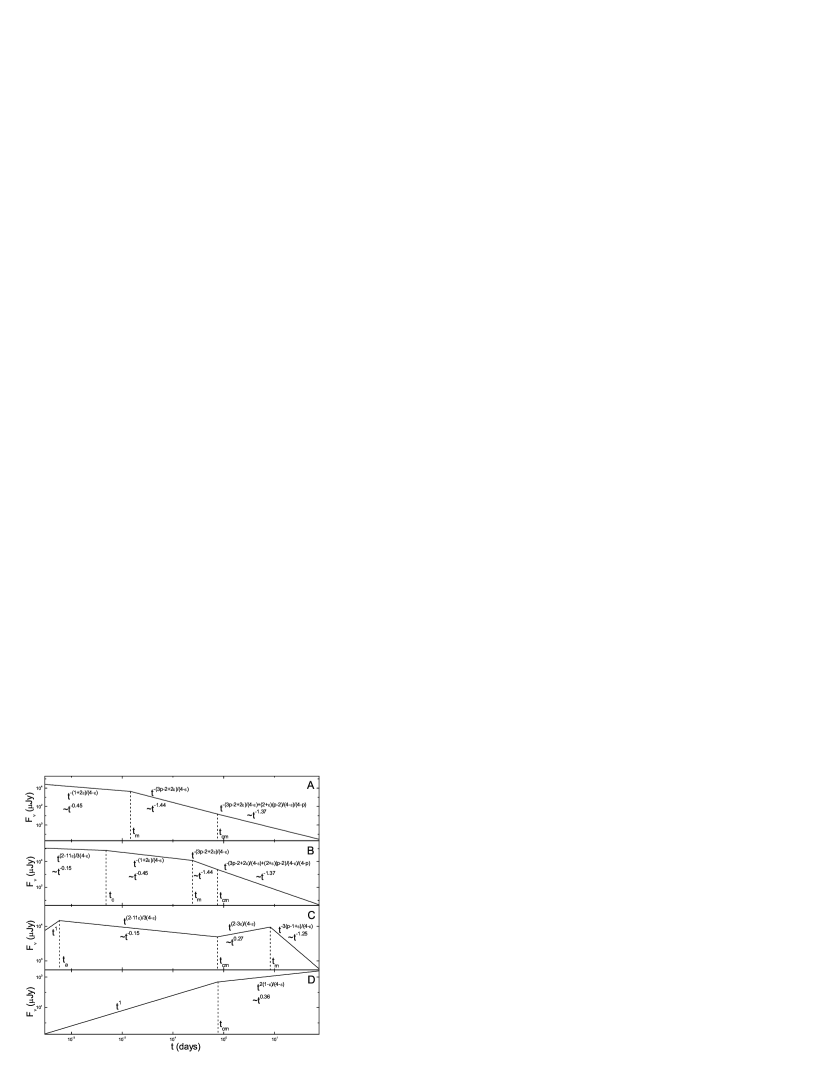
Figure 1: Characteristic afterglow light curves from a semi-radiative blast wave in an interstellar medium (ISM) in various frequency ranges. The panels are ordered from high frequency (type A) to low frequency (type D). X-ray and optical light curves are typically of types A and B, while sub-millimeter and radio light curves are typically of types C and D. The physical parameters for these light curves are $E_{cm}=10^{53}$ ergs, $n=1$ cm^-3, $\epsilon=\epsilon_{e}=1/3$, $\epsilon_{B}=10^{-2.5}$, $p=2.2$. The event is assumed to be at redshift of $z=1$.

In the case of ISM, the orders of these times are (A) $t_{c}<t_{a}<t_{m}<t_{cm}$ for $\nu>\nu_{ac}$; (B) $t_{a}<t_{c}<t_{m}<t_{cm}$ for $\nu_{cm}<\nu<\nu_{ac}$; (C) $t_{a}<t_{cm}<t_{m}<t_{c}$ for $\nu_{a}(t_{cm})<\nu<\nu_{cm}$; (D) $t_{cm}<t_{a}<t_{m}<t_{c}$ for $\nu<\nu_{a}(t_{cm})$. Here $\nu_{a}(t_{cm})$ is the SSA frequency at $t_{cm}$. Using the equations (29), (30), and (61) in the case of $k=0$, the light curves in each case can be constructed as (A) $F_{\nu}\propto t^{1}\nu^{2}$ ($t<t_{c}$), $F_{\nu}\propto t^{(5-2\epsilon)/(4-\epsilon)}\nu^{5/2}$ ($t_{c}$, $t_{a}$), $F_{\nu}\propto t^{-(1+2\epsilon)/(4-\epsilon)}\nu^{-1/2}$ ($t_{a}$, $t_{m}$), $F_{\nu}\propto t^{-(3p-2+2\epsilon)/(4-\epsilon)}\nu^{-p/2}$ ($t_{m}$, $t_{cm}$), $F_{\nu}\propto t^{-(3p-2+2\epsilon)/(4-\epsilon)+(2+\epsilon)(p-2)/(4+\epsilon)/(4-p)}\nu^{-p/2}$ ($t>t_{cm}$); (B) $F_{\nu}\propto t^{1}\nu^{2}$ ($t<t_{a}$), $F_{\nu}\propto t^{(2-11\epsilon)/3(4-\epsilon)}\nu^{1/3}$ ($t_{a}$, $t_{c}$), $F_{\nu}\propto t^{-(1+2\epsilon)/(4-\epsilon)}\nu^{-1/2}$ ($t_{c}$, $t_{m}$), $F_{\nu}\propto t^{-(3p-2+2\epsilon)/(4-\epsilon)}\nu^{-p/2}$ ($t_{m}$, $t_{cm}$), $F_{\nu}\propto t^{-(3p-2+2\epsilon)/(4-\epsilon)+(2+\epsilon)(p-2)/(4+\epsilon)/(4-p)}\nu^{-p/2}$ ($t>t_{cm}$); (C) $F_{\nu}\propto t^{1}\nu^{2}$ ($t<t_{a}$), $F_{\nu}\propto t^{(2-11\epsilon)/3(4-\epsilon)}\nu^{1/3}$ ($t_{a}$, $t_{cm}$), $F_{\nu}\propto t^{(2-3\epsilon)/(4-\epsilon)}\nu^{1/3}$ ($t_{cm}$, $t_{m}$), $F_{\nu}\propto t^{-3(p-1+\epsilon)/(4-\epsilon)}\nu^{-(p-1)/2}$ ($t_{m}$, $t_{c}$), $F_{\nu}\propto t^{-(3p-2+2\epsilon)/(4-\epsilon)+(2+\epsilon)(p-2)/(4+\epsilon)/(4-p)}\nu^{-p/2}$ ($t>t_{c}$); (D) $F_{\nu}\propto t^{1}\nu^{2}$ ($t<t_{cm}$), $F_{\nu}\propto t^{2(1-\epsilon)/(4-\epsilon)}\nu^{2}$ ($t_{cm}$, $t_{a}$), $F_{\nu}\propto t^{(2-3\epsilon)/(4-\epsilon)}\nu^{1/3}$ ($t_{a}$, $t_{m}$), $F_{\nu}\propto t^{-3(p-1+\epsilon)/(4-\epsilon)}\nu^{-(p-1)/2}$ ($t_{m}$, $t_{c}$), $F_{\nu}\propto t^{-(3p-2+2\epsilon)/(4-\epsilon)+(2+\epsilon)(p-2)/(4+\epsilon)/(4-p)}\nu^{-p/2}$ ($t>t_{c}$). The light curves in the ISM case are illustrated in Figure 1. The crossing times $t_{c}$ and $t_{a}$ in case A and $t_{a}$ in case B occur very early in high observing frequencies, while $t_{c}$ in case C and $t_{a}$, $t_{m}$ and $t_{c}$ in case D occur very late in low observing frequencies. We thus neglect these crossing times in the figure. As indicated in Figure 1, the radiation efficiency, $\epsilon$, has a marked effect on the afterglow light curves. It changes the temporal decaying index $\alpha$ (defined as $F_{\nu}\propto t^{-\alpha}$) of the light curve significantly. For illustration, we adopt $\epsilon=\epsilon_{e}=1/3$ and $p=2.2$ in the following. The initial slowly increasing light curve segment, $F_{\nu}\propto t^{1/6}$, predicted in the standard adiabatic blast wave model will changes to be a slowly decreasing one, $F_{\nu}\propto t^{(2-11\epsilon)/3(4-\epsilon)}\sim t^{-0.15}$, as shown in the early segment of case C. This makes the sub-millimeter afterglow less competitive to distinguish between the ISM and the stellar wind, as proposed by Panaitescu & Kumar (2000), if the observations are not frequent enough. At the optical wavelength, the early light curve behaves typically as $F_{\nu}\propto t^{-(1+2\epsilon)/(4-\epsilon)}\sim t^{-0.45}$ rather than $F_{\nu}\propto t^{-1/4}$ in the adiabatic case. When $\nu_{m}$ crosses the observing frequency, i.e. $t>t_{m}$, the optical and X-ray light curves decays as $F_{\nu}\propto t^{-(3p-2+2\epsilon)/(4-\epsilon)}\sim t^{-1.44}$, as shown in cases B and A. It should be noted that many X-ray afterglow light curves and a considerable fraction of optical afterglow light curves have temporal decaying indices steeper than predicted $(3p-2)/4\sim 1.15$ by the standard adiabatic model (for $p\approx 2.2$). The observed decaying indices in the X-ray afterglow light curves are $\langle\alpha_{X}\rangle=1.33\pm 0.38$, while the median value of the observed X-ray spectral indices $\beta_{X}$, $F_{\nu}\propto\nu^{-\beta_{X}}$, is $\sim 1.05$ (Berger, Kulkarni, & Frail 2003; De Pasquale et al. 2003). Assuming the X-ray frequency is above the cooling frequency and the spectral index is $\beta_{X}=p/2$, the measured $p$ is consistent with the standard value of the index of electron energy distribution, $p=2.2-2.3$, predicted in the relativistic shock acceleration mechanism (see Achterberg et al. 2001 and reference therein). However, the observed mean temporal decaying index $\langle\alpha_{X}\rangle$ requires a relatively larger $\langle p\rangle$, $\sim 2.44$, provided the shock is adiabatic. There are several caveats on the observations of the X-ray afterglows. First, the temporal behavior of the X-ray afterglow is hardly influenced by the equal arrival time surface effect, which will mix the earlier light from high latitudes into the present light. This effect is important especially for high observing frequencies, e.g. the optical and X-ray. The profile of surface emissivity of the relativistic shock is ring-like in these high frequencies (Sari 1998). This will moderately slow down the decreasing rate of the afterglow after $t_{m}$ for the theoretical light curve A. However, the X-ray afterglow is immune to this effect because its $t_{m}$ is very early and the observed decreasing index $\alpha_{X}$ is based on the observations typically several hours after the burst. Second, the measured $\beta_{X}$ is reliable since the X-ray absorption in the medium along the line of sight takes place at $\nu\lesssim 1$ keV while the observing window is $\sim 2-10$ keV. Lastly, one should be cautious when interpreting the property of X-ray afterglow with the synchrotron radiation mechanism, because the X-ray afterglow may be contaminated by the synchrotron-self-Compton component. However, there have so far been only a few X-ray afterglows that were confirmed to have the IC components. Therefore, the radiative corrections to the afterglow light curves must be taken into account based on the observations. As can be seen in Figure 1, the light curve at high frequency (type A and B) flattens when the afterglow enters the slow-cooling phase, $t>t_{cm}$. At the transition time $t_{cm}$, the spectrum nearby the observing frequency changes from $\nu_{c}<\nu_{m}<\nu$ to $\nu_{m}<\nu_{c}<\nu$, while the expressions for the flux density are the same, i.e. $F_{\nu}=F_{\nu,\max}\nu_{m}^{(p-1)/2}\nu_{c}^{1/2}\nu^{-p/2}$. The flattening of the light curve results from the Compton parameter $Y$ in the flux density, i.e. $F_{\nu}\propto Y^{-1}$, since $\nu_{c}\propto(1+Y)^{-2}\approx Y^{-2}$. The Compton parameter $Y$ in the slow-cooling phase decreases slowly, contrary to its constancy in the earlier fast-cooling phase. From equation (54) for $Y$ in the slow-cooling phase and adopting $k=0$, the change of the temporal index around $t_{cm}$ is $\Delta\alpha=(2+\epsilon)(p-2)/[(4-\epsilon)(4-p)]$, which is shown in the last segments of panels A and B in Figure 1. Note that since Sari et al. (1998) did not discuss IC cooling, there is no related segment in their $\epsilon=0$ light curves.

In the case of stellar wind, the orders of the crossing times are (A) $t_{a}<t_{m}<t_{cm}<t_{c}$ for $\nu>\nu_{cm}$; (B) $t_{a}<t_{c}<t_{cm}<t_{m}$ for $\nu_{ac}<\nu<\nu_{cm}$; (C) $t_{c}<t_{a}<t_{cm}<t_{m}$ for $\nu_{a}(t_{cm})<\nu<\nu_{ac}$; (D) $t_{c}<t_{cm}<t_{a}<t_{m}$ for $\nu<\nu_{a}(t_{cm})$. Using the equations (29), (30), and (61) in the case of $k=2$, the light curves in each case can be constructed as (A) $F_{\nu}\propto t^{(7-5\epsilon)/2(2-\epsilon)}\nu^{5/2}$ ($t<t_{a}$), $F_{\nu}\propto t^{-(1+\epsilon)/2(2-\epsilon)}\nu^{-1/2}$ ($t_{a}$, $t_{m}$), $F_{\nu}\propto t^{-[3p-2-(p-2)\epsilon]/2(2-\epsilon)}\nu^{-p/2}$ ($t_{m}$, $t_{cm}$), $F_{\nu}\propto t^{-[3p-2-(p-2)\epsilon]/2(2-\epsilon)+(p-2)/(4-p)}\nu^{-p/2}$ ($t_{cm}$, $t_{c}$), $F_{\nu}\propto t^{-[3p-1-(p-1)\epsilon]/2(2-\epsilon)}\nu^{-(p-1)/2}$ ($t>t_{c}$); (B) $F_{\nu}\propto t^{(7-5\epsilon)/2(2-\epsilon)}\nu^{5/2}$ ($t<t_{a}$), $F_{\nu}\propto t^{-(1+\epsilon)/2(2-\epsilon)}\nu^{-1/2}$ ($t_{a}$, $t_{c}$), $F_{\nu}\propto t^{-(4-\epsilon)/3(2-\epsilon)}\nu^{1/3}$ ($t_{c}$, $t_{cm}$), $F_{\nu}\propto t^{-\epsilon/3(2-\epsilon)}\nu^{1/3}$ ($t_{cm}$, $t_{m}$), $F_{\nu}\propto t^{-[3p-1-(p-1)\epsilon]/2(2-\epsilon)}\nu^{-(p-1)/2}$ ($t>t_{m}$); (C) $F_{\nu}\propto t^{(7-5\epsilon)/2(2-\epsilon)}\nu^{5/2}$ ($t<t_{c}$), $F_{\nu}\propto t^{(4-3\epsilon)/(2-\epsilon)}\nu^{2}$ ($t_{c}$, $t_{a}$), $F_{\nu}\propto t^{-(4-\epsilon)/3(2-\epsilon)}\nu^{1/3}$ ($t_{a}$, $t_{cm}$), $F_{\nu}\propto t^{-\epsilon/3(2-\epsilon)}\nu^{1/3}$ ($t_{cm}$, $t_{m}$), $F_{\nu}\propto t^{-[3p-1-(p-1)\epsilon]/2(2-\epsilon)}\nu^{-(p-1)/2}$ ($t>t_{m}$); (D) $F_{\nu}\propto t^{(7-5\epsilon)/2(2-\epsilon)}\nu^{5/2}$ ($t<t_{c}$), $F_{\nu}\propto t^{(4-3\epsilon)/(2-\epsilon)}\nu^{2}$ ($t_{c}$, $t_{cm}$), $F_{\nu}\propto t^{2(1-\epsilon)/(2-\epsilon)}\nu^{2}$ ($t_{cm}$, $t_{a}$), $F_{\nu}\propto t^{-\epsilon/3(2-\epsilon)}\nu^{1/3}$ ($t_{a}$, $t_{m}$), $F_{\nu}\propto t^{-[3p-1-(p-1)\epsilon]/2(2-\epsilon)}\nu^{-(p-1)/2}$ ($t>t_{m}$). The light curves in the stellar wind case are illustrated in Figure 2. The crossing time $t_{c}$ in cases C and D occurs very early at low observing frequency, while $t_{m}$ in case D occurs very late. We neglect these crossing times in this figure. The radiation efficiency has a significant effect on the light curves in the wind case. The flux density in the optical/infrared light curve decays initially with $t^{-(1+\epsilon)/2(2-\epsilon)}\sim t^{-0.4}$, rather than $t^{-1/4}$ in the adiabatic case, which is shown in case A. For the X-ray afterglow the crossing time $t_{m}$ when the typical frequency $\nu_{m}$ crosses the observing frequency is much earlier, the light curve behaves as $t^{-[3p-2-(p-2)\epsilon]/2(2-\epsilon)}\sim t^{-1.36}$ during the whole fast-cooling phase, which is more consistent with observations than the adiabatic light curve (Berger, Kulkarni, & Frail 2003). The light curve at high frequency flattens when the afterglow transits to the slow-cooling phase. By the same way as in the ISM case, from equation (54) for $Y$ and adopting $k=2$, the change of the temporal index around $t_{cm}$ is $\Delta\alpha=(p-2)/(4-p)$ in the wind case. Since Chevalier & Li (2000) did not include IC cooling, there is no relevant flattening segment in their $\epsilon=0$ light curves. Although the flattening of the optical/X-ray light curve around $t_{cm}$ predicted in the inverse Compton dominated cooling regime in the stellar wind case is more obvious than in the ISM case, the change of the temporal decaying index is only $\Delta\alpha\sim 0.1$ for the former case. The detailed theoretical optical light curves taking into account the equal arrival time surface effect and the large error bars in X-ray afterglow observations prevent us from the identifications of such flattening.

5 Conclusions and Discussion

In this paper, we have investigated analytically the GRB afterglow hydrodynamics and constructed the semi-radiative light curves realistically. We focus on the case that the electron cooling is in the inverse Compton dominated regime, i.e. $\epsilon_{e}\gg\epsilon_{B}$ or $Y\gg 1$. The realistic hydrodynamics is applicable for spherical blast waves with the assumption that the electron energy equipartition factor $\epsilon_{e}$ is not much larger than $1/3$, which seems to be reasonable based on theoretical expectations and observations as well. In fact, the analytical solution for afterglow hydrodynamics is almost tenable throughout the relativistic stage when $\epsilon_{e}\lesssim 2/3$ (see equation 2). The only uncertainty is the actual evolution of the radiation efficiency in the late slow-cooling phase. Given $p\sim 2.2-2.3$, we conclude that a constant radiation efficiency is a good approximation for a fairly long time in the slow-cooling phase. The transition from fast-cooling to slow-cooling happens much later in the IC dominated cooling regime than in the purely synchrotron cooling regime. Since the actual radiation efficiency decreases very slowly in the slow-cooling phase, the semi-radiative epoch is further prolonged typically by two orders of magnitude in time, other than the whole fast-cooling phase as commonly used. As the GRB ejecta sweeps up more and more external medium, the Lorentz factor $\gamma$ of the shock decreases. When $\gamma$ equals the inverse of the initial half-opening angle $\theta_{0}$ of the GRB conical ejecta, or jet, the following afterglow light curves deviate from the previously spherical-like ones, and the light curves in this paper are not suitable at this late stage. Generally, our semi-radiative afterglow light curves hold true when the shock is relativistic after the initial deceleration time and before the jet-like stage, with the radiation efficiency satisfying $\epsilon\approx\epsilon_{e}\lesssim$max$\{\displaystyle\frac{2}{2+\theta_{0}},\frac{2}{3}\}$.

The adiabatic afterglow light curves in the synchrotron dominated cooling regime have been well studied in previous works (Sari et al. 1998; Chevalier & Li 2000; Granot & Sari 2002). Sari et al. (1998) have considered the light curves of a fully radiative ($\epsilon=1$) blast wave. However, our analytical results can not be directly applied to this case. Actually, in the fully radiative case, equation (2) can also be directly integrated and the hydrodynamics and the resulting light curves are the same as derived by Sari et al. (1998). The radiative corrections to the afterglow light curves in the wind model have been discussed by Chevalier & Li (2000). They had adopted the scaling laws of a semi-radiative shock given by Böttcher & Dermer (2000). The temporal exponents of the hydrodynamics and light curves in Böttcher & Dermer (2000) differ from ours. In fact, the radiation corrections for these exponents in their work are smaller than that in our work. Cohen, Piran & Sari (1998) had studied the hydrodynamics of a semi-radiative relativistic blast wave considering a more complicated post-shock material distribution (similar to Blandford & McKee 1976) than that of the simple thin-shell approximation as in our work. However, the hydrodynamic evolution differs in all these three treatments of Cohen et al. (1998), Böttcher & Dermer (2000) and this paper. The hydrodynamic self-similarity index $m$ we obtain lies between the other two’s. Despite the difference between the hydrodynamics due to different approximations/treatments, we can see that the radiative corrections to afterglow light curves are significant. For example, the temporal decaying index of X-ray afterglows at around $10$ hours since the main bursts varies in the range of $1.23-1.69$ in the ISM case, and $1.21-1.58$ in the stellar wind case for $p=2.2-2.3$ and $\epsilon_{e}=0.1-0.5$, provided that the IC component is neglected. This range is consistent with the observations (Berger, Kulkarni & Frail 2003). In observations, the value of $\epsilon_{e}$ and $p$ can be inferred for a particular X-ray afterglow from the so called “closure relation” between the temporal index $\alpha_{X}$ and spectral index $\beta_{X}$, provided that the IC component can be neglected. Such a closure relation can be obtained from case A described in §4 in either ISM or wind cases. The application of this method to optical afterglows should be cautious. The early optical light curve has a broken power law profile around $t_{m}$. In contrary to the early X-ray afterglow whose $t_{m}$ is much earlier and which can be regarded as a simple power law one, the optical light curve might be affected moderately when the equal arrival time surface effect is included. Another reason is that the reddening in optical spectra is unknown. While the Galactic extinction can be empirically decoupled, the extinction and reddening within the circum-burst environment and host galaxy are less constrained. These two facts prevent the credible measurements of the temporal and spectral indices of optical afterglows, respectively.

We have got the criteria for the emergence of IC components in soft X-ray afterglows, through giving the lower limits of external medium densities. In the ISM case, the lower limit of $n$ is $\sim 10$ cm^-3 in the fast-cooling phase, while it is $\sim 1$ cm^-3 in the slow-cooling phase (Panaitescu & Kumar 2000; Sari & Esin 2001; Zhang & Mészáros 2001). These are typical densities of interstellar media in our galaxy. In the wind case, the lower limit of the wind parameter is always $A_{\ast}\sim 1$ (Panaitescu & Kumar 2000). Such a critical $A_{\ast}$ is also typical for Wolf-Rayet stars in our galaxy. It should be noted that the wind parameter obtained from fitting afterglows within the wind interaction model seems to be quite small (Chevalier & Li 1999, 2000; Panaitescu & Kumar 2001; Dai & Wu 2003; Chevalier, Li, & Fransson 2004). The contradiction may be due to the limitation of our knowledge about the mass losses of massive stars at the last stage before their collapses. Taking the inferred low $A_{\ast}$ from afterglows, we draw a tentative conclusion that the IC components in X-ray afterglows are insignificant in the stellar wind case. For such a low $A_{\ast}$, a wind bubble would be produced and surrounded by either an outer giant molecular cloud, a slow wind at previous evolutionary stage, or an extremely high pressure in a star-burst environment (Dai & Wu 2003; Chevalier, Li, & Fransson 2004). The termination shock radius of the wind bubble will be reached by the GRB shock within hours in observer’s frame. The environment of the shock will change from wind type to uniform medium type after this time. We have neglected such a complicated case in this work. Recently, Yost et al. (2003) had relaxed the assumption of a constant magnetic equipartition factor $\epsilon_{B}$ and broadened the circum-burst medium types. They had made a detailed comparison between the results of different assumptions as well as different circum-burst media, and found the degeneracy of different assumed evolutions of $\epsilon_{B}$ and different medium types. Anyway, we adopt the constant $\epsilon_{B}$ assumption and consider the most possible medium types, i.e. the ISM and the stellar wind.

The radiative corrections in modelling afterglows are important. Such an effect should be taken into account seriously in analysis of afterglows, especially when a large number of afterglows will be observed in the Swift era. It will affect directly the energetics of GRB remnants and therefore the actual efficiency of prompt GRBs (Wu et al. in preparation, which also includes the ICS effect).

We thank the referee for his/her valuable suggestions and comments. This work was supported by the National Natural Science Foundation of China (grants 10233010, 10221001, 10003001, and 10473023), the Ministry of Science and Technology of China (NKBRSF G19990754), the Special Funds for Major State Basic Research Projects, and the Foundation for the Author of National Excellent Doctoral Dissertation of P. R. China (Project No. 200125).

Figure 2: Characteristic afterglow light curves from a semi-radiative blast wave in a stellar wind in various frequency ranges. The panels are ordered from high frequency (type A) to low frequency (type D). X-ray, optical, and infrared light curves are typically of type A, sub-millimeter light curve is typically of type B, while radio light curve is typically of types C and D. The physical parameters for these light curves are $E_{cm}=10^{53}$ ergs, $A_{\ast}=1$, $\epsilon=\epsilon_{e}=1/3$, $\epsilon_{B}=10^{-2.5}$, $p=2.2$. The event is assumed to be at redshift of $z=1$.

References

- Achterberg et al. (2001) Achterberg, A., Gallant, Y. A., Kirk, J. G., & Guthmann, A. W. 2001, MNRAS, 328, 393
- Berger, Kulkarni & Frail (2003) Berger, E., Kulkarni, S. R., & Frail, D. A. 2003, ApJ, 590, 379
- Björnsson (2001) Björnsson, C. I. 2001, ApJ, 554, 593
- Blandford & McKee (1976) Blandford, R. D., & McKee, C. F. 1976, Phys. Fluids, 19, 1130
- Böttcher & Dermer (2000) Böttcher, M., & Dermer, C. D. 2000, ApJ, 532, 281
- Cheng & Lu (2001) Cheng, K. S., & Lu, T. 2001, ChJAA, 1, 1
- Chevalier & Li (1999) Chevalier, R. A., & Li, Z. Y. 1999, ApJ, 520, L29
- Chevalier & Li (2000) Chevalier, R. A., & Li, Z. Y. 2000, ApJ, 536, 195
- Chevalier, Li & Fransson (2004) Chevalier, R. A., Li, Z. Y., & Fransson, C. 2004, ApJ, 606, 369
- Cohen et al. (1998) Cohen, E., Piran, T., & Sari, R. 1998, ApJ, 509, 717
- Dai & Lu (1998) Dai, Z. G., & Lu, T. 1998, MNRAS, 298, 87
- Dai & Lu (1999) Dai, Z. G., & Lu, T. 1999, ApJ, 519, L155
- Dai & Lu (2000) Dai, Z. G., & Lu, T. 2000, ApJ, 537, 803
- Dai & Wu (2003) Dai, Z. G., & Wu, X. F. 2003, ApJ, 591, L21
- Dermer Böttcher & Chiang (2000) Dermer, C. D., Böttcher, M., & Chiang, J. 2000, ApJ, 537, 255
- De Pasquale et al. (2003) De Pasquale, M., et al. 2003, ApJ, 592, 1018
- Feng et al. (2002) Feng, J. B., Huang, Y. F., Dai, Z. G., & Lu, T. 2002, ChJAA, 2, 525
- Galama et al. (1998) Galama, T. J., et al. 1998, Nature, 395, 670
- Galama et al. (1998) Galama, T. J., Wijers, R. A. M. J., Bremer, M., Groot, P. J., Strom, R. G., Kouveliotou, C., & van Paradijs, J. 1998, ApJ, 500, L97
- Granot & Sari (2002) Granot, J., & Sari, R. 2002, ApJ, 568, 820
- Hjorth et al. (2003) Hjorth, J., et al. 2003, Nature, 423, 847
- Huang et al. (1999) Huang, Y. F., Dai, Z. G., & Lu, T. 1999, MNRAS, 309, 513
- Huang et al. (2000) Huang, Y. F., Gou, L. J., Dai, Z. G., & Lu, T. 2000, ApJ, 543, 90
- Kulkarni et al. (1998) Kulkarni, S. R., et al. 1998, Nature, 395, 663
- Li et al. (2002) Li, Z., Dai, Z. G., & Lu, T. 2002, MNRAS, 330, 955
- Lloyd-Ronning & Zhang (2004) Lloyd-Ronning, N. M., & Zhang, B. 2004, ApJ, 613, 477
- Mészáros, & Rees (1997) Mészáros, P., & Rees, M. 1997, ApJ, 476, 232
- Mészáros, Rees & Wijers (1998) Mészáros, P., Rees, M., & Wijers, R. A. M. J. 1998, ApJ, 499, 301
- Mészáros (2002) Mészáros, P. 2002, ARA&A, 40, 137
- Paczyński (1998) Paczyński, B. 1998, ApJ, 494, L45
- Panaitescu & Kumar (2000) Panaitescu, A., & Kumar, P. 2000, ApJ, 543, 66
- Panaitescu & Kumar (2001) Panaitescu, A., & Kumar, P. 2001, ApJ, 560, L49
- Panaitescu & Kumar (2002) Panaitescu, A., & Kumar, P. 2002, ApJ, 571, 779
- Piran (2004) Piran, T. 2004, Rev. Mod. Phys., in press (astro-ph/0405503)
- Sari, Piran & Narayan (1998) Sari, R., Piran, T., & Narayan, R. 1998, ApJ, 497, L17
- Sari (1998) Sari, R. 1998, ApJ, 494, L49
- Sari & Esin (2001) Sari, R., & Esin, A. A. 2001, ApJ, 548, 787
- Stanek et al. (2003) Stanek, K. Z., et al. 2003, ApJ, 591, L17
- Van Paradijs et al. (2000) Van Paradijs, J., Kouveliotou, C., & Wijers, R. A. M. J. 2000, ARA&A, 38, 379
- Vietri (1997) Vietri, M. 1997, ApJ, 478, L9
- Wang et al. (2001) Wang, X. Y., Dai, Z. G., & Lu, T. 2001, ApJ, 556, 1010
- Waxman (1997) Waxman, E. 1997, ApJ, 485, L5
- Wijers, Rees & Mészáros (1997) Wijers, R. A. M. J., Rees, M. J, & Mészáros, P. 1997, MNRAS, 288, L51
- Wei & Lu (1998) Wei, D. M., & Lu, T. 1998, ApJ, 505, 252
- Wei & Lu (2000) Wei, D. M., & Lu, T. 2000, A&A, 360, L13
- Wooley (1993) Woosley, S. E. 1993, ApJ, 405, 273
- Wu et al. (2003) Wu, X. F., Dai, Z. G., Huang, Y. F., & Lu, T. 2003, MNRAS, 342, 1131
- Yost et al. (2003) Yost, S. A., Harrison, F. A., Sari, R., & Frail, D. A. 2003, ApJ, 597, 459
- Zhang & Mészáros (2001) Zhang, B., & Mészáros, P. 2001, ApJ, 559, 110
- Zhang & Mészáros (2004) Zhang, B., & Mészáros, P. 2004, Int. J. Mod. Phys. A, 19, 2385