Large scale inhomogeneity and local dynamical friction

We investigate the effect of a density gradient on Chandrasekhar’s dynamical friction formula based on the method of 2-body encounters in the local approximation. We apply these generalizations to the orbit evolution of satellite galaxies in Dark Matter haloes. We find from the analysis that the main influence occurs through a position-dependent maximum impact parameter in the Coulomb logarithm, which is determined by the local scale-length of the density distribution. We also show that for eccentric orbits the explicit dependence of the Coulomb logarithm on position yields significant differences for the standard homogeneous force. Including the velocity dependence of the Coulomb logarithm yields ambigous results. The orbital fits in the first few periods are further improved, but the deviations at later times are much larger. The additional force induced by the density gradient, the inhomogeneous force, is not antiparallel to the satellite motion and can exceed 10% of the homogeneous friction force in magnitude. However, due to the symmetry properties of the inhomogeneous force, there is a deformation and no secular effect on the orbit at the first order. Therefore the inhomogeneous force can be safely neglected for the orbital evolution of satellite galaxies. For the homogeneous force we compare numerical N-body calculations with semi-analytical orbits to determine quantitatively the accuracy of the generalized formulae of the Coulomb logarithm in the Chandresekhar approach. With the local scale-length as the maximum impact parameter we find a significant improvement of the orbital fits and a better interpretation of the quantitative value of the Coulomb logarithm.

1 Introduction

Dynamical friction has a wide range of applications in stellar-dynamical systems. It appears as the first order term in the Fokker-Planck approximation (see e.g. Binney & Tremaine bin87 (1987), hereafter BT, Eq. (8-53)) competing with the second order diffusion terms to allow for a Maxwellian as the equilibrium distribution. In the field of relaxation processes (dissolution of star clusters, gravo-thermal collapse, mass segregation) the physical constraints and dominating aspects of dynamical friction are very different to those of the dynamical evolution of a single massive body in a sea of light background particles. In the latter case the friction force is independent of the mass of the background particles, and as long as the massive body is far from energy equipartition the diffusion can be neglected. Its main applications are the satellite galaxies in the dark matter halo (DMH) of their parent galaxy, and super-massive black holes (SMBH) or compact star clusters in the central bulge region of galaxies. Even in a collisional gas, dynamical friction occurs, but corrections due to pressure forces must be applied (Just et al. jus86 (1986); Just & Kegel jus90 (1990); Ostriker ost99 (1999) using mode analysis, and Sánchez-Salcedo & Brandenburg san99 (1999, 2001) using numerical calculations).

There are different approaches to analyse the parameter dependence and to calculate the magnitude of the friction force, most of them based on perturbative methods (2-body collisions: Chandrasekhar cha43 (1943); Binney bin77 (1977); Spitzer spi87 (1987); BT; mode analysis: Marochnik mar68 (1968); Kalnajs kal72 (1972); Tremaine & Weinberg tre84 (1984); theory of linear response: Colpi et al. col99 (1999); statistical correlations in the fluctuating field: Maoz mao93 (1993)). Due to its complicated structure, dynamical friction shows many different features. In a recent theoretical investigation Nelson & Tremaine (nel99 (1999)) connected many physical aspects of the fluctuating gravitational field on the basis of the linear response theory. For practical applications one basic question is whether dynamical friction acting on a massive object is dominated by local processes. There is a longstanding discussion on the contribution of global modes to dynamical friction, which are known to be excited and enhanced by the self-gravity of the perturbation (Weinberg wei86 (1986, 1989, 1993); Hernquist & Weinberg her89 (1989)). These strong resonances may reduce the dissipation rate considerably (Kalnajs kal72 (1972); Tremaine & Weinberg tre84 (1984); Weinberg wei89 (1989)), but see also Rauch & Tremaine (rau96 (1996)) for the opposite effect. For interacting galaxies with moderate mass ratios, the global deformation of the main galaxy and the strong tidal forces on the perturber can enhance the energy and momentum loss by considerable factors, which cannot be described by the Chandrasekhar dynamical friction form (Prugniel & Combes pru92 (1992); Leeuwin & Combes lee97 (1997) and the discussion therein). The mass of the perturber should not exceed $\sim 5\%$ of the mass of the host object in order to neglect both the global contribution to the dynamical friction force and the effect of deformation.

This paper is concerned with the local contribution to dynamical friction. We restrict our analysis to the low mass regime with $M<0.05\,M_{\rm h}$, where $M$ and $M_{\rm h}$ are the mass of the perturber and the host object, respectively. For clearness we formulate most equations in terms of the orbital motion of satellite galaxies in the DMH of the parent galaxy and give additionally the explicit application to a singular isothermal halo. This case will also be used for the numerical analysis. Nevertheless the results can be used for more general background distributions with isotropic distribution functions and also for compact objects. As a second application we give the corresponding equations for massive Black Holes moving in galactic centres.

The basic formula of Chandrasekhar relies on an infinite homogeneous background with an isotropic velocity distribution function. For a Maxwellian velocity distribution function and a massive object with $M\gg m$ it is given by

$$\@vec{\dot{v}_{\rm hom}} = -C_{\rm Ch}G_{\rm hom}(X)\@vec{e_{\rm v_{\rm M}}}\quad\mbox{with}$$ (1)

$$G_{\rm hom}(X) = \frac{\ln\Lambda}{X^{2}}\left[erf(X)-\frac{2X}{\sqrt{\pi}}\exp(-X^{2})\right]\quad,$$

$$C_{\rm Ch} = \frac{2\pi G^{2}\rho_{0}M}{\sigma^{2}}\quad\mbox{and}\quad X=\frac{|v_{\rm M}|}{\sqrt{2}\sigma}$$ (2)

(BT Eqs. (7-14), (7-18)). Here $M$ and $v_{\rm M}$ are mass and velocity of the massive body; $m$, $\rho_{0}$, and $\sigma$ are mass, mass density, and velocity dispersion of the ambient particles, respectively. In this formula, only 2-body interactions between the massive particle and the background are included, adopting a straight-line motion in the unperturbed potential. Essentially all uncertainties of the relevant regime in phase space for these 2-body encounters are hidden in the Coulomb logarithm $\ln\Lambda$. Different perturbation methods lead to different interpretations of $\Lambda$: (1) 2-body encounters: $\Lambda=b_{\rm max}/b_{\rm min}$ with maximum and minimum impact parameter (BT) (2) Mode analysis: $\Lambda=k_{\rm max}/k_{\rm min}$ with maximum and minimum relevant wavenumber (Kalnajs kal72 (1972)) (3) Theory of linear response: $\Lambda=\tau_{\rm max}/\tau_{\rm min}$ with maximum and minimum time lag of the correlations (Nelson & Tremaine nel99 (1999)). The most important correction to Eq. 1 is due to an anisotropic velocity distribution (Binney bin77 (1977); Statler sta88 (1988, 1991)). A numerical investigation of the anisotropy is discussed in another paper for satellite motion in flattened Dark Matter haloes (Peñarrubia pen03 (2003); Peñarrubia et al. pen04 (2004)). In different approaches the inhomogeneity of the background distribution is generally included (Kalnajs kal72 (1972); Tremaine & Weinberg tre84 (1984); Colpi et al. col99 (1999); Nelson & Tremaine nel99 (1999)) but a useful scheme for applications is not yet available. An explicit formula for corrections due to the local density gradient is given by Binney (bin77 (1977)), who has shown that the additional inhomogeneous force can be neglected for the dynamics of galaxies in galaxy clusters. Maoz (mao93 (1993)) and follow-up papers ( Sánchez-Salcedo san99a (1999); Dominguez-Teneiro & Gómez-Flechoso dom98 (1998)) used the fluctuation-dissipation theory with approximations similar to those presented here to derive the energy loss due to dynamical friction. Del Popolo & Gambera (pop99 (1999)) and Del Popolo (pop03 (2003)) compute the corrections due to a density enhancement spherically symmetric with respect to the massive body, which may be used to estimate the shielding effect on the friction force.

Numerical calculations suffered for a long time from resolution problems (e.g. Lin & Tremaine lin83 (1983); White whi83 (1983); Bontekoe & van Albada bon87 (1987); Weinberg wei93 (1993)) and, even in recent years, computations with particle numbers below $10^{5}$ are frequently used (Cora et al. cor97 (1997); van den Bosch et al. bos99 (1999); Jiang & Binney jia00 (2000); Hashimoto et al. has03 (2003)). Low resolution raises two major problems for the determination of orbital decay times and quantitative numbers for the Coulomb logarithm $\ln\Lambda$. Due to noise, the numerically determined Coulomb factors $\Lambda$ vary significantly for the same orbits. With different seeds and evolution times for relaxation of the unperturbed galaxy using 5,000 particles Cora et al. (cor97 (1997)) found a variation of fitted values for $\Lambda$ by almost a factor of 3. Even in the 20,000 particle runs the single orbits differ by up to a factor of 2 in the satellite energy. Secondly, increasing the resolution should lead to systematically larger values for the Coulomb logarithm, because the range of impact parameters, where the perturbation of the motion of the background particles is resolved, increases. This is explicitely shown in Spinnato et al. (spi03 (2003)). Therefore even an average over many low resolution computations underestimates the friction force and leads to too large decay times for the satellite galaxies. With the new generation of computers it is now possible to perform a larger number of self-consistent calculations with particle numbers above $10^{6}$ and the corresponding high grid resolutions in particle-mesh codes (Velázquez & White vel99 (1999); Peñarrubia et al. pen02 (2002); Spinnato et al. spi03 (2003)). In these calculations one can hope to suppress noise sufficiently and to also resolve the small scale perturbations to model the full range for the Coulomb logarithm. Bertin et al. (ber03 (2003)) also used a large number of particles but only a low spatial resolution due to the restriction on low order spherical harmonics. For the excitation of resonant global modes in N-body calculations, one order of magnitude higher particle numbers may be necessary. But this is not our aim here.

The standard usage of Chandrasekhar’s formula works with an individual fitting of the constant Coulomb logarithm for each orbit. Fitting the Coulomb logarithm to a single orbit provides in most cases an accurate description of a large part of the orbit. For this task, there is no need to improve the method. But the Coulomb logarithm varies systematically from orbit to orbit as discussed above and the orbital fits drift away for long-living satellites (Lin & Tremaine lin83 (1983); Jiang & Binney jia00 (2000); Spinnato et al. spi03 (2003); Peñarrubia et al. pen04 (2004)). In order to get an improved friction formula, which can be used for a sample of orbits with different parameters, we apply local constraints yielding a systematic variation of the Coulomb logarithm with position (and also velocity). The distance to the galactic centre as the maximum impact parameter for the orbital evolution of the Magellanic Clouds was already proposed by Tremaine (tre76 (1976)) and a position-dependent Coulomb logarithm was found numerically by Bontekoe & van Albada (bon87 (1987)) and Bertin et al. (ber03 (2003)). However the properties of a position-dependent $\ln\Lambda$ were never investigated systematically. We discuss also the velocity dependence of $\Lambda$ by excluding slow encounters.

A second effect of the local density gradient of the background distribution is an additional ’inhomogeneous’ force. Due to the different symmetry of the density gradient, the net effect of the perpendicular component of 2-body encounters does not vanish like that for the homogeneous part, but leads to an additional force not anti-parallel to the satellite motion (see also Binney bin77 (1977)). We discuss the new Coulomb logarithm and the inhomogeneous friction term in detail.

We calculate dynamical friction using the explicit deflection of 2-body encounters, because this approach is not based on the diffusion limit in phase space. Therefore, in the case of a massive particle, the derivation also holds for large angle deflections leading to a well-defined behaviour for small impact parameters and slow encounters. Neglecting the effect of the mean tidal field on the encounter yields the well known deflection

$$\@vec{\Delta v_{\rm M\|}} = \frac{2m\@vec{V_{\rm 0}}}{M}\left[1+\frac{b^{2}V_{\rm 0}^{4}}{G^{2}M^{2}}\right]^{-1}$$ (3)

$$= \frac{2Gm}{a(V_{\rm 0})}\frac{\@vec{V_{\rm 0}}}{V_{\rm 0}^{2}}\left[1+\frac{b^{2}}{a(V_{\rm 0})^{2}}\right]^{-1}\,,$$

$$\@vec{\Delta v_{\rm M\bot}} = \frac{2m\@vec{b}V_{\rm 0}^{3}}{GM^{2}}\left[1+\frac{b^{2}V_{\rm 0}^{4}}{G^{2}M^{2}}\right]^{-1}$$ (5)

$$= \frac{2Gm\@vec{b}}{a(V_{\rm 0})^{2}V_{\rm 0}}\left[1+\frac{b^{2}}{a(V_{\rm 0})^{2}}\right]^{-1}$$

$$\qquad\mbox{with}\qquad a(V_{\rm 0})=\frac{GM}{V_{\rm 0}^{2}}$$

(BT, Eqs. (7-10a,b)) for a given impact parameter $\@vec{b}$ and relative velocity $\@vec{V_{\rm 0}}$. Here $a(V_{\rm 0})$ corresponds to the impact parameter for a $90^{\circ}$ deflection. From this acceleration we have to subtract the acceleration along the unperturbed orbit properly in order to avoid artificial results due to differences in the mean field approximation.

We start in Sect. 2 with a detailed discussion of the collision rate of 2-body encounters and the structure of the Coulomb logarithm with all parameter dependences. In Sect. 3 we compute the inhomogeneous dynamical friction for an isotropic distribution function including a reanalysis of the homogeneous friction force (corresponding to the standard friction) for a consistent comparison of both parts. In Sects. 4 and 5 we apply the new formulae to typical satellite orbits in the Dark Matter halo of the Milky Way and discuss the effect of the improved Coulomb logarithm and of the inhomogeneous friction term. Sect. 6 contains a discussion of the relevance of using a position-dependent Coulomb logarithm and of the inhomogeneous force for other applications (super massive black holes in galactic cores) and other aspects (circularization of the orbits).

2 Encounter rates and the Coulomb logarithm

In this section we discuss the encounter rate and perform the integration over impact parameters for the homogeneous and the inhomogeneous contribution to dynamical friction. General symmetries of the force and the properties of the Coulomb logarithm are described in detail.

2.1 Encounter rate and mean field correction

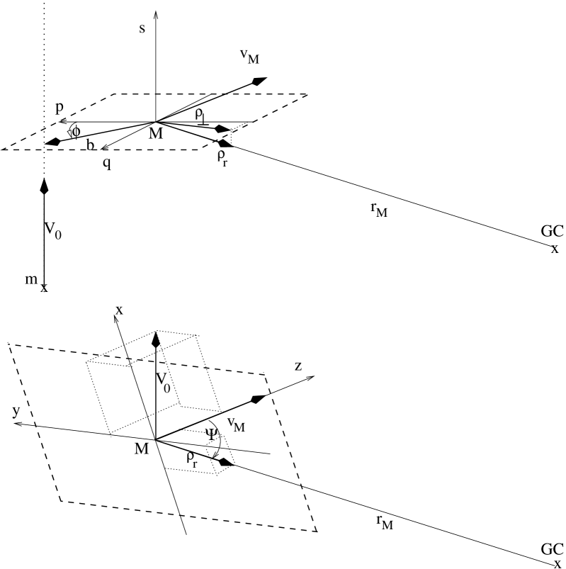
Figure 12: Upper panel: Coordinate system centred at $M$ (position $\@vec{r_{\rm M}}$) oriented parallel to $\@vec{V_{\rm 0}}$ for integration over impact parameter. Lower panel: Coordinate system centred at $M$ oriented parallel to $\@vec{v_{\rm M}}$ for integration over velocity space $\mbox{\rm d}^{3}V_{\rm 0}$.

We use a local coordinate system $(p,q,s)$ with $s$ parallel to $\@vec{V_{\rm 0}}$ and $(p,q)$ the plane of impact parameters perpendicular to $\@vec{V_{\rm 0}}$ (see Fig. 12). The integration over $s$ is substituted by the encounter rate $n(r)|\@vec{V_{\rm 0}}|$ with unperturbed background density $n(r)$ and with $\@vec{r}=\@vec{r_{\rm M}}+\@vec{b}$ using formally a 3-dimensional impact parameter in vectorial form, if necessary, given by $\@vec{b}=(p,q,0)=b(\cos\phi,\sin\phi,0)$. The rate of encounters for given relative velocity $\@vec{V_{\rm 0}}$ and impact parameter $\@vec{b}$ is then

$$\mbox{\rm d}\nu(\@vec{b},\@vec{V_{\rm 0}})=|\@vec{V_{\rm 0}}|n(\@vec{r})f(\@vec{v})\mbox{\rm d}p\mbox{\rm d}q\mbox{\rm d}^{3}V_{\rm 0}\,,$$ (6)

the Dark Matter particles are counted when they are crossing the $(p,q)$-plane. The density gradient parallel to $\@vec{V_{\rm 0}}$ corresponds to an acceleration due to the mean field because the phase space density along (unperturbed) orbits is constant at equilibrium. The effect on the timing during the encounter can be accounted for only when tidal fields are taken into account. Accelerations due to the mean field will not be included here. The density gradient perpendicular to $\@vec{V_{\rm 0}}$ changes the encounter rate directly. This effect of the local inhomogeneity is dominant and will be included.

Since we are interested in the additional acceleration due to the grainy structure of the background distribution, we have to take the difference of the acceleration between the perturbed and the unperturbed orbit. Particles moving along the unperturbed orbits with impact parameter $\@vec{b}$ and relative velocity $\@vec{V_{\rm 0}}$ correspond to a ’line’ of constant density $\rho(\@vec{r})f(\@vec{v})\mbox{\rm d}s\mbox{\rm d}p\mbox{\rm d}q\mbox{\rm d}^{3}V_{\rm 0}$ along $s$, that is, parallel to $V_{\rm 0}$. By symmetry, only the parallel component to $\@vec{b}$ contributes. We find

$$\@vec{\dot{v}_{\rm M0}} = \int G\rho(\@vec{r})f(\@vec{v})\int_{-\infty}^{\infty}\frac{\@vec{b}\mbox{\rm d}s}{\sqrt{b^{2}+s^{2}}^{3}}\mbox{\rm d}p\mbox{\rm d}q\mbox{\rm d}^{3}V_{\rm 0}$$ (7)

$$= \quad\int\frac{2G\rho(\@vec{r})\@vec{b}}{b^{2}}f(\@vec{v})\mbox{\rm d}p\mbox{\rm d}q\mbox{\rm d}^{3}V_{\rm 0}$$

for the acceleration along the unperturbed motion. This acceleration must be subtracted from the acceleration due to 2-body encounters yielding an effective acceleration due to the grainy structure of the Dark Matter given by

$$\@vec{\dot{v}_{\rm df}}=\int\@vec{\Delta v_{\rm M}}\mbox{\rm d}\nu(b,V_{\rm 0})-\@vec{\dot{v}_{\rm M0}}\equiv\@vec{\dot{v}_{\rm M\|}}+\@vec{\dot{v}_{\rm M\bot}}\quad.$$ (8)

Since the correction due to the unperturbed orbits is parallel to $\@vec{b}$, it affects only the perpendicular component. We find from Eqs. 3 and 5

$$\@vec{\dot{v}_{\rm M\|}} = \int\frac{2G\rho(\@vec{r})f(\@vec{v})}{a(V_{\rm 0})}\frac{\@vec{V_{\rm 0}}}{V_{\rm 0}}\left[1+\frac{b^{2}}{a(V_{\rm 0})^{2}}\right]^{-1}\mbox{\rm d}p\mbox{\rm d}q\mbox{\rm d}^{3}V_{\rm 0}\,,$$ (9)

$$\@vec{\dot{v}_{\rm M\bot}} = \int\left(\frac{2G\rho(\@vec{r})f(\@vec{v})\@vec{b}}{a(V_{\rm 0})^{2}}\left[1+\frac{b^{2}}{a(V_{\rm 0})^{2}}\right]^{-1}\right.$$

$$\quad\left.-\frac{2G\rho(\@vec{r})f(\@vec{v})\@vec{b}}{b^{2}}\right)\mbox{\rm d}p\mbox{\rm d}q\mbox{\rm d}^{3}V_{\rm 0}$$

$$= \int\frac{-2G\rho(\@vec{r})f(\@vec{v})\@vec{b}}{b^{2}}\left[1+\frac{b^{2}}{a(V_{\rm 0})^{2}}\right]^{-1}\mbox{\rm d}p\mbox{\rm d}q\mbox{\rm d}^{3}V_{\rm 0}\,.$$

For the integration over the impact parameters we expand the local density distribution up to the first order in the $(p,q)$-plane

$$\rho(r)\approx\rho_{0}+\@vec{b}\cdot\@vec{\rho_{\rm\bot}}\quad\mbox{with}\quad\@vec{r}=\@vec{r_{\rm M}}+\@vec{b}\quad.$$ (11)

Here $\rho_{0}=\rho(\@vec{r})|_{\rm r_{\rm M}}$ and for the local density gradient we use the abbreviations

$$\@vec{\rho_{r}} \equiv \nabla\rho(\@vec{r})|_{r_{\rm M}}\equiv\left(\rho_{x},\rho_{y},\rho_{z}\right)\equiv\left(\rho_{p},\rho_{q},\rho_{s}\right)\quad\mbox{and}\quad$$ (12)

$$\@vec{\rho_{\rm\bot}} = \@vec{\rho_{r}}-(\@vec{\rho_{r}}\cdot\@vec{e_{\rm V_{\rm 0}}})\@vec{e_{\rm V_{\rm 0}}}=(\rho_{p},\rho_{q},0)$$ (13)

with coordinate systems $(x,y,z)$ oriented to the velocity of the satellite with $z$ axis parallel to $\@vec{v_{\rm M}}$, and $(p,q,s)$ with $s$ axis parallel to $\@vec{V_{\rm 0}}$ (both are locally centred at $\@vec{r_{\rm M}}$, see Fig. 12). The vector $\@vec{\rho_{\rm\bot}}$ is the component of the density gradient perpendicular to $\@vec{V_{\rm 0}}$. In the Taylor expansion an additional variation of $f(\@vec{v})$ is neglected. So, for example, we do not account for some spatial variation of the velocity dispersion $\sigma(r)$.

2.2 Symmetries and general properties

There are two important features of the velocity change due to 2-body encounters: The symmetries and the mass dependence. Both are fundamentally different for the parallel and the perpendicular component.

$\@vec{\Delta v_{\rm M\|}}$: In the limit of small angle deflections ($b\gg a(V_{\rm 0})$) the parallel component is proportional to the mass $M$ leading to the well known mass segregation. This also easily allows a separation from mean field effects.

The parallel component is a function of $b^{2}$ only. Therefore, in a local Taylor expansion of the distribution function, only terms even in $p$ and in $q$ contribute to the integral over the impact parameters. These are the constant term, and diagonal terms of second derivatives, and so on.

The parallel component is odd in $V_{\rm 0}$. Therefore the contribution vanishes for vanishing satellite velocity $v_{\rm M}$, if the distribution function $f(\@vec{v})$ is symmetric.

$\@vec{\Delta v_{\rm M\bot}}$: For small angles the perpendicular acceleration is proportional to $M^{2}$ leading to a stronger mass dependence. On the other hand, the acceleration falls off more steep with $V_{\rm 0}$ leading to a dominating contribution at small $V_{\rm 0}$.

The perpendicular component is odd in $\@vec{b}$, therefore terms odd in $p$ or $q$ in the Taylor expansion of the distribution function contribute to the integral over the impact parameters, i.e. the linear term, $3^{\rm rd}$ derivative terms, …

The perpendicular component is even in $V_{\rm 0}$. This has the effect of a net acceleration also for vanishing $v_{\rm M}$ due to the asymmetric gravitational wake.

Note that these symmetries are relative to the velocity $\@vec{V_{\rm 0}}$ and not to the velocity $\@vec{v_{\rm M}}$ of the satellite through the Dark Matter. The directions of the accelerations relative to $v_{\rm M}$ depend on the symmetries of the distribution function $f(\@vec{v})$. The zeroth order (parallel component), that is the standard Chandrasekhar friction, is only parallel to $v_{\rm M}$ for an isotropic distribution function. The first order (the dominating term of the perpendicular component) is not perpendicular to $v_{\rm M}$ even for an isotropic distribution function. For vanishing $v_{\rm M}$ and isotropic velocity distribution function it is antiparallel to the density gradient. This is equivalent to an effective reduction of the enclosed mass ${\cal M}(r_{\rm M})$ of the Dark Matter halo.

2.3 Integration over the impact parameters

Before integrating over the impact parameters we shall discuss the minimum and maximum impact parameter interpretation.

Minimum impact parameter $b_{0}$: For compact objects the minimum impact parameter is irrelevant if $b_{0}\ll a(V_{\rm 0})$. In this case $b_{0}$ can be set to zero, but for a unified formulation we will use the Schwarzschild radius in the case of a Black hole. Since $M\gg m$, even in the case of large angle deflections, the velocity change $\Delta\@vec{v_{\rm M}}$ is small and can be handled as a perturbation (i.e. under validity of using superposition of 2-body encounters). For extended bodies, there is an additional effective $b_{0}$ determined by the typical radius of the satellite. The half-mass radius $r_{h}$ is a good choice with a correction factor of order unity, because the deflection angle is dominated by the force near the minimum distance and is determined by the enclosed mass. For a Plummer sphere the half-mass radius is given by $r_{h}=GM/(4.6\sigma_{0}^{2})=1.3r_{c}$ with a central velocity dispersion $\sigma_{0}$ and core radius $r_{c}$ (the detailed calculation of White (whi76 (1976)) corresponds to $b_{0}=1.6r_{c}$). An analytic calculation for extended bodies is given by Mulder (mul83 (1983)). For a King profile the half-mass radius is between 1/3 and 1/4.6 of $GM/\sigma_{0}^{2}$, again with central velocity dispersion $\sigma_{0}$ of the satellite. Therefore we use for extended objects

$$b_{0}=r_{h}\approx\frac{GM}{4\sigma_{0}^{2}}\quad.$$ (14)

The latter approximation, which also corresponds to the half-mass radius of a singular isothermal sphere with outer cut-off, will be used for the investigation of the parameter dependence of the Coulomb logarithm. In case of a compact object, we use a characteristic radius for $b_{0}$ (the Schwarzschild radius $r_{S}$ for a Black Hole) and define the corresponding virtual velocity dispersion by $\sigma_{0}^{2}=GM/4b_{0}$ leading for a BH to

$$b_{0}=r_{S}=\frac{2GM}{c^{2}}=\frac{GM}{4\sigma_{0}^{2}}\quad\mbox{with}\quad\sigma_{0}^{2}\equiv\frac{GM}{4b_{0}}=\frac{c^{2}}{8}$$ (15)

in order to get a consistent description.

Maximum impact parameter $b_{1}$: The allowed (and effective) range of impact parameters is bounded by the geometry and by the relevant time-scales. The local approximation of the distribution function in density (and possibly in velocity space also) breaks down for distances larger than the local scale-length $L$. Therefore the maximum impact parameter should be smaller than $L$,

$$b<L\equiv\rho/|\nabla\rho|=\rho_{0}/|\@vec{\rho_{r}}|\quad.$$ (16)

By using this cut-off, we neglect more distant encounters and may underestimate dynamical friction. For a singular isothermal sphere we have $L=r_{\rm M}/2$. We account for this uncertainty by using a fitting factor $Q_{2}$ in the maximum impact parameter.

The straight-line approximation and the local approximation require that the encounter time $t_{\rm coll}=2b/V_{\rm 0}$ is short compared to the local dynamical time-scale $t_{\rm dyn}$, which is essentially determined by the local crossing time of the satellite $t_{\rm dyn}=L/v_{\rm M}$

$$\frac{2b}{V_{\rm 0}}=t_{\rm coll}<t_{\rm dyn}=\frac{L}{v_{\rm M}}\quad.$$ (17)

So the maximum impact parameter depends on $V_{\rm 0}$. Using normalized velocities $X=v_{\rm M}/(\sqrt{2}\sigma)$ and $W=V_{\rm 0}/(\sqrt{2}\sigma)$, it is given by

$$b_{1}=Q_{2}L\,min[1,\frac{V_{\rm 0}}{2v_{\rm M}}]\approx Q_{2}L\sqrt{\frac{W^{2}}{4X^{2}+W^{2}}}\quad.$$ (18)

In order to guarantee formally $b_{1}>b_{0}$ also for very small $V_{\rm 0}$ we will use the analytic approximation

$$b_{1}^{2}=b_{0}^{2}+Q_{2}^{2}L^{2}\frac{W^{2}}{4X^{2}+W^{2}}\quad.$$ (19)

Since again it is a priori not clear whether the time-scale restriction does not exclude an important contribution of long-term encounters, we will also carry out computations using a maximum impact parameter given by

$$b_{1}^{2}=b_{0}^{2}+Q_{1}^{2}L^{2}\quad,$$ (20)

neglecting the time-scale argument.

2.4 Homogeneous and inhomogeneous dynamical friction

For clarity we split the dynamical friction $\@vec{\dot{v}_{\rm df}}$ (Eq. 8) into the part induced by the homogeneous density term and that by the local density gradient (inhomogeneous friction)

$$\@vec{\dot{v}_{\rm df}}\equiv\@vec{\dot{v}_{\rm hom}}+\@vec{\dot{v}_{\rm inh}}\quad.$$ (21)

By symmetry, one has that after integrating over the impact parameters, only the parallel component $\@vec{\dot{v}_{\rm M\|}}$ contributes to the homogeneous friction $\@vec{\dot{v}_{\rm hom}}$, and the perpendicular component $\@vec{\dot{v}_{\rm M\bot}}$ to the inhomogeneous friction $\@vec{\dot{v}_{\rm inh}}$. For comparison we calculate the standard case (homogeneous part, parallel component) in the same way as the inhomogeneous term. Inserting into Eq. 9 the Taylor expansion of the density (Eq. 11) and integrating over impact parameters gives (the gradient term vanish by symmetry after integration over angle $\phi$ from $\mbox{\rm d}p\mbox{\rm d}q=\mbox{\rm d}\phi b\mbox{\rm d}b$)

$$\@vec{\dot{v}_{\rm hom}} = \int f(\@vec{v})\frac{2G\rho_{0}\@vec{V_{\rm 0}}}{a(V_{\rm 0})V_{\rm 0}}\int_{\rm b_{0}^{2}}^{b_{1}^{2}}\left[1+\frac{b^{2}}{a(V_{\rm 0})^{2}}\right]^{-1}\pi\mbox{\rm d}b^{2}\mbox{\rm d}^{3}V_{\rm 0}$$ (22)

$$= 4\pi G\rho_{0}\int\frac{\@vec{V_{\rm 0}}}{V_{\rm 0}}a(V_{\rm 0})\ln(\Lambda)f(\@vec{v})\mbox{\rm d}^{3}V_{\rm 0}$$

with

$$\Lambda=\sqrt{\left.\left(1+\frac{b_{1}^{2}}{a(V_{\rm 0})^{2}}\right)\right/\left(1+\frac{b_{0}^{2}}{a(V_{\rm 0})^{2}}\right)}\quad.$$ (23)

The inhomogeneous term arises from the leading contribution of the perpendicular acceleration and gives the dominant contribution to the acceleration perpendicular to $\@vec{V_{\rm 0}}$. The integration over the angle $\phi$ leads to

$$\int_{0}^{2\pi}(\@vec{b}\cdot\@vec{\rho_{\rm\bot}})\@vec{b}\mbox{\rm d}\phi=\pi b^{2}\@vec{\rho_{\rm\bot}}\quad.$$ (24)

Using this result for the integration of Eq. LABEL:vbot0 over the impact parameters we find

$$\@vec{\dot{v}_{\rm inh}} = -\int\pi G\@vec{\rho_{\rm\bot}}f(\@vec{v})\int_{\rm b_{0}^{2}}^{b_{1}^{2}}\left[1+\frac{b^{2}}{a(V_{\rm 0})^{2}}\right]^{-1}\mbox{\rm d}b^{2}\mbox{\rm d}^{3}V_{\rm 0}$$ (25)

$$= -2\pi G\int\@vec{\rho_{\rm\bot}}a(V_{\rm 0})^{2}\ln(\Lambda)f(\@vec{v})\mbox{\rm d}^{3}V_{\rm 0}\quad,$$

where only the density gradient term of the Taylor expansion contributes. Note that $\@vec{\rho_{\rm\bot}}$, the density gradient perpendicular to $\@vec{V_{\rm 0}}$, is a function of $\@vec{V_{\rm 0}}$ leading to a more complicated angular integral in velocity space.

2.5 The Coulomb logarithm

Figure 1: The different approximations for the Coulomb logarithm as a function of normalized encounter velocity $W=V_{\rm 0}/(\sqrt{2}\sigma)$. The full, dotted and dashed lines show $\ln(\Lambda_{2})$ (see Eq. 28) for different normalized satellite velocities $X=v_{\rm M}/(\sqrt{2}\sigma)$. The satellite parameters $q_{\rm d}=40,q_{\rm s}=5$ correspond to a mass of $M=5.6\cdot 10^{9}M_{\rm\odot}$ at a distance of $r_{\rm M}=40$ kpc in a Milky Way-like halo. For comparison the Coulomb logarithm $\ln(\Lambda_{1})$ (see Eq. 30, dashed-dotted line) is shown. The corresponding value for a Coulomb logarithm independent of the encounter velocity $\ln(\Lambda_{0})$ (see Eq. 33, thin line) is also plotted. We have chosen $Q_{0}=0.8$ and $Q_{2}=2.5$ from the numerical experiments and the corresponding value $Q_{1}=1.0$, which leads to the same friction force for $X=1$.

For the analysis of the parameter dependence of the Coulomb logarithm, we can reformulate Eq. 23 using two scaling parameters, namely the size ratio $q_{\rm d}$ and the ratio of specific kinetic energies $q_{\rm s}$ defined by

$$q_{\rm d}=\frac{L}{b_{0}}\qquad q_{\rm s}=\frac{\sigma^{2}}{\sigma_{0}^{2}}\quad,$$ (26)

instead of the dependence on $b_{0}$, $b_{1}$, and the mass $M$. Since $\sigma_{0}$ is very large for compact objects (see Eq. 15), we get very small values for $q_{\rm s}$, which can in most cases be neglected. With Eq. 14, Eq. 5 becomes

$$a(V_{\rm 0})=\frac{GM}{V_{\rm 0}^{2}}=\frac{2b_{0}}{q_{\rm s}W^{2}}\quad.$$ (27)

With Eqs. 19 and 23 we get the analytic approximation

$$\ln\Lambda_{2} = \ln\sqrt{\frac{1+\frac{W^{4}}{4}q_{\rm s}^{2}\left(1+Q_{2}^{2}q_{\rm d}^{2}\frac{W^{2}}{W^{2}+4X^{2}}\right)}{1+\frac{W^{4}}{4}q_{\rm s}^{2}}}$$ (28)

$$\leadsto Q_{2}^{2}q_{\rm d}^{2}q_{\rm s}^{2}\frac{W^{6}}{32X^{2}}\quad\mbox{for}\quad W\leadsto 0$$ (29)

and alternatively with Eq. 20

$$\ln\Lambda_{1} = \ln\sqrt{\frac{1+\frac{W^{4}}{4}q_{\rm s}^{2}\left(1+Q_{1}^{2}q_{\rm d}^{2}\right)}{1+\frac{W^{4}}{4}q_{\rm s}^{2}}}$$ (30)

$$\leadsto Q_{1}^{2}q_{\rm d}^{2}q_{\rm s}^{2}\frac{W^{4}}{8}\quad\mbox{for}\quad W\leadsto 0\quad.$$ (31)

In order to isolate the effect of the dependence on the encounter velocity $W$ of the Coulomb logarithm, we also analyse $\ln\Lambda_{0}$ independent of $W$ by using the position-dependent maximum impact parameter $b_{1}=Q_{0}L$ and an estimation $a_{90}$ of the typical impact parameter for a $90^{\circ}$ deflection. With $(V_{0}^{2})_{\rm typ}=2\sigma^{2}+v_{\rm M}^{2}$ inserted into Eq. 5 we find

$$a_{90}\equiv\frac{GM}{2\sigma^{2}+v_{\rm M}^{2}}=\frac{2b_{0}}{q_{\rm s}(1+X^{2})}\quad,$$ (32)

which depends on $r_{\rm M}$ and $v_{\rm M}$, but not on $W$. Inserting this into Eq. 23, we find

$$\ln\Lambda_{0} = \ln\frac{Q_{0}L}{\sqrt{r_{\rm h}^{2}+a_{90}^{2}}}=\ln\frac{Q_{0}q_{\rm d}}{\sqrt{1+4q_{\rm s}^{-2}(1+X^{2})^{-2}}}$$ (33)

$$\approx \ln(Q_{0}q_{\rm d})\qquad\quad\qquad\mbox{\rm for extended objects}$$ (34)

$$\approx \ln\frac{Q_{0}L(2\sigma^{2}+v_{\rm M}^{2})}{GM}\quad\mbox{\rm for compact objects.}$$ (35)

For the fits to the numerical orbits we also use a globally constant value $\langle\ln\Lambda\rangle$.

In the case of an isothermal halo we can substitute $q_{\rm d}$ by using ${\cal M}(r_{\rm M})$, the enclosed DMH mass, and the mass $M$ of the satellite, where

$$L=\frac{r_{\rm M}}{2} {\cal M}(r_{\rm M})=4\pi\rho r_{\rm M}^{3}=\frac{2\sigma^{2}r_{\rm M}}{G}$$ (36)

$$q_{\rm m} = \frac{{\cal M}(r_{\rm M})}{M}=q_{\rm s}q_{\rm d}\quad.$$ (37)

For the isothermal halo the Coulomb logarithm becomes

$$\ln\Lambda_{2}=\ln\sqrt{\frac{1+\frac{W^{4}}{4}\left(q_{\rm s}^{2}+Q_{2}^{2}q_{\rm m}^{2}\frac{W^{2}}{W^{2}+4X^{2}}\right)}{1+\frac{W^{4}}{4}q_{\rm s}^{2}}}\quad,$$ (38)

and similar for $\ln\Lambda_{1}$. In Fig. 1 the velocity dependence of the Coulomb logarithm is shown for different satellite velocities $X$ and typical parameters $q_{\rm d},q_{\rm s}$ ($X=1$ corresponds to a circular orbit in an isothermal halo). We show the velocity-dependent Coulomb logarithm $\ln(\Lambda_{2})$ for $X=0.1;\,1.0;\,3.0$ (dotted, full, and dashed line). We have chosen $Q_{2}=2.5$, which is the best fit value for typical orbits discussed below. For smaller $X$ the cut-off at low relative velocities $W$ is steeper, whereas for higher $X$ it becomes flatter. The Coulomb logarithm $\ln(\Lambda_{1})$ (dashed-dotted line) with constant $b_{\rm max}$ shows a shallower cut-off for $W\rightarrow 0$ ($\propto W^{4}$ for $W^{2}\ll 2/q_{\rm s}$ instead of $\propto W^{6}$ for $W^{2}\ll 2/q_{\rm s}$ and $W^{2}\ll 4X^{2}$), which occurs at a lower relative velocity. In general, the cut-off shifts the main contribution to the friction force to higher values of $W$. For the simpler approximation $\ln(\Lambda_{1})$ we used $Q_{1}=1.0$ in order to get the same force for $X=1$ after integration over $W$. Neglecting the velocity dependence by using $\ln(\Lambda_{0})$ with the best fit value $Q_{0}=0.9$(thin line) leads to the corresponding constant value for comparison. The effect of the low velocity cut-off on the friction force is discussed in detail in Sect. 3.

3 The dynamical friction force

For the integration over velocity space we restrict the analysis to the isotropic velocity distribution functions $f(v^{2})$. An anisotropy plus a local density gradient would lead to very complicated angle integrations, which can hardly be performed analytically. All details of the integrations in spherical coordinates in $\mbox{\rm d}^{3}V_{\rm 0}$-space are given in the Appendix. Here we discuss the results of a Gaussian distribution

$$f(v^{2}) = \frac{1}{(\sqrt{2\pi}\sigma)^{3}}\exp(-\frac{v^{2}}{2\sigma^{2}})$$ (39)

for the explicit integration, but the general results do not depend strongly on the special shape of $f(v^{2})$ and it can be done in the same way for other functions.

The homogeneous friction vector $\@vec{\dot{v}_{\rm hom}}$ is parallel to the satellite motion $\@vec{v_{\rm M}}$, whereas the inhomogeneous friction lies in the $(\@vec{v_{\rm M}},\@vec{\rho_{r}})$-plane with angle $\Psi$ between $\@vec{v_{\rm M}}$ and $\@vec{\rho_{r}}$. Therefore we decompose the inhomogeneous term into the parallel and orthogonal components with respect to $\@vec{v_{\rm M}}$

$$\@vec{\dot{v}_{\rm inh}} \equiv \@vec{\dot{v}_{\rm par}}+\@vec{\dot{v}_{\rm ort}}\quad\mbox{with}\quad$$

$$\qquad\@vec{\dot{v}_{\rm par}}=(\@vec{\dot{v}_{\rm inh}}\cdot\@vec{e_{\rm v_{\rm M}}})\@vec{e_{\rm v_{\rm M}}}$$

$$\qquad\@vec{\dot{v}_{\rm ort}}=|\@vec{\dot{v}_{\rm ort}}|\@vec{e_{\rm ort}}\quad.$$

It is convenient to use the normalized functions $G_{\rm hom}(X)$, $G_{\rm par}(X)$, and $G_{\rm ort}(X)$

$$G_{\rm hom}(X)=\frac{2}{\sqrt{\pi}}\int_{0}^{\infty}\ln(\Lambda)\exp(-W^{2}-X^{2})\times$$

$$\quad\left[\cosh(2WX)-\frac{\sinh(2WX)}{2WX}\right]\frac{\mbox{\rm d}W}{WX}\quad,$$ (41)

$$G_{\rm par}(X)=\frac{2}{\sqrt{\pi}q_{\rm d}q_{\rm s}}\int_{\rm 0}^{\infty}\ln(\Lambda)\exp(-W^{2}-X^{2})\times$$

$$\quad\left[\cosh(2WX)-\frac{\sinh(2WX)}{2WX}\right]\frac{\mbox{\rm d}W}{X^{2}W^{4}}\quad,$$ (42)

$$G_{\rm ort}(X)=\frac{1}{\sqrt{\pi}q_{\rm d}q_{\rm s}}\int_{\rm 0}^{\infty}\ln(\Lambda)\exp(-W^{2}-X^{2})\times$$

$$\quad\left[\sinh(2WX)\frac{4W^{2}X^{2}+1}{2WX}-\cosh(2WX)\right]\frac{\mbox{\rm d}W}{X^{2}W^{4}}$$ (43)

leading to

$$\@vec{\dot{v}_{\rm hom}} = -C_{\rm Ch}G_{\rm hom}(X)\@vec{e_{\rm v_{\rm M}}}\quad,$$ (44)

$$\@vec{\dot{v}_{\rm par}} = -C_{\rm Ch}G_{\rm par}(X)\cos(\Psi)\@vec{e_{\rm v_{\rm M}}}\quad,$$ (45)

$$\@vec{\dot{v}_{\rm ort}} = -C_{\rm Ch}G_{\rm ort}(X)\sin(\Psi)\@vec{e_{\rm ort}}\quad,$$ (46)

where the projection factors $\cos(\Psi)$ and $\sin(\Psi)$ of the density gradient (see Eq. 62) are separated. The scaling factor $1/(q_{\rm d}q_{\rm s})$ ($=1/q_{\rm m}$ for an isothermal halo) is included in the functions $G_{\rm par}(X)$, $G_{\rm ort}(X)$. The explicit derivation of these functions are given in the Appendix (see Eq. 77). In a spherical halo the radial and tangential components $\@vec{\dot{v}_{\rm r}},\@vec{\dot{v}_{\rm t}}$ of the inhomogeneous friction are

$$\@vec{\dot{v}_{\rm r}} = C_{\rm Ch}\left[G_{\rm ort}(X)\cos^{2}(i)+G_{\rm par}(X)\sin^{2}(i)\right]\@vec{e_{\rm r}}\quad,$$ (47)

$$\@vec{\dot{v}_{\rm t}} = -C_{\rm Ch}\left[G_{\rm ort}(X)-G_{\rm par}(X)\right]\sin(i)\cos(i)\@vec{e_{\rm t}}$$ (48)

with inclination $i$ of $\@vec{\rm v_{\rm M}}$ with respect to $\@vec{e_{\rm t}}$.

3.1 Homogeneous dynamical friction

Here we shall discuss the effect of retaining the dependence of $\Lambda$ on the encounter velocity $W$. Neglecting $W$ in the logarithmic term introduces an error of about 20% (see Fig. 2) in the friction force, which is a function of $X$. The velocity dependence on $\ln\Lambda$ is twofold. The natural cut-off for large angle encounters due to the reduced efficiency is included in both approximations, $\ln\Lambda_{1}$ and $\ln\Lambda_{2}$. In $\ln\Lambda_{2}$ additionally the slow encounter cut-off in the maximum impact parameter (see Eq. 19) is included. The effect of these dependences can best be seen by comparing with the friction force using $\ln\Lambda_{0}$ (Eq. 33) with velocity independent maximum impact parameter $b_{1}$ and an average impact parameter $a_{90}$ for the $90^{\circ}$ deflection. $\ln\Lambda_{0}$ is still position and orbit dependent via $L$, $\sigma$, and $v_{\rm M}$.

Figure 2: Relative homogeneous friction forces as a function of satellite velocity $X$ for the different approximations of the Coulomb logarithm. The thin line shows the friction force $G_{\rm hom}$ using $\ln\Lambda_{0}$ for orientation. The other lines give the relative variation $G_{\rm hom}(\Lambda_{1})/G_{\rm hom}(\Lambda_{0})$ and $G_{\rm hom}(\Lambda_{2})/G_{\rm hom}(\Lambda_{0})$, respectively, for two sets of parameters $q_{\rm d}$, $q_{\rm s}$. The first case is for a satellite galaxy, whereas the second case corresponds to a point-like object (SMBH with $M=2\,10^{7}M_{\odot}$).

In Fig. 2 the force ratios using $\ln\Lambda_{1}$ or $\ln\Lambda_{2}$ with respect to $\ln\Lambda_{0}$ are plotted as a function of satellite velocity $X$ for different satellite parameters. The typical range of $X$ for eccentric orbits is $0.5<X<2$. For an orientation the thin line gives the normalized friction force $G_{\rm hom}$ using $\ln\Lambda_{0}$. All other lines show the ratio of $G_{\rm hom}$ using $\ln\Lambda_{1}$ or $\ln\Lambda_{2}$ with respect to that using $\ln\Lambda_{0}$. We can learn three things from this plot. Firstly, the variation is below 20% for all parameter sets. Therefore for a determination of the magnitude of the dynamical friction force, the simple generalization $\ln\Lambda_{0}$ in the Chandrasekhar formula will work well. Secondly, the systematic variation between apo- and peri-centre depends on the approximation and on the parameters. This means that for a detailed investigation of the evolution of satellite systems or of the circularization, it may be necessary to include the explicit velocity dependence in the Coulomb logarithm. Thirdly, there is a significant relative variation of the strength of the forces along eccentric orbits. The ratio of the forces at apo- and peri-centre can differ by 30%, when using $\ln\Lambda_{0}$ instead of $\ln\Lambda_{1}$ or $\ln\Lambda_{2}$. Since the amount of circularization of the orbit depends on the relative strength of the forces around apo- and peri-centre (see Sect. 5.1), this may lead to essential differences in the orbital evolution of satellite galaxies. In Sects. 4 and 5 we give some numerical examples to show that the new approximations of the Coulomb logarithm improve the orbital fits.

3.2 Inhomogeneous dynamical friction

The properties of the inhomogeneous force given in Eqs. 45 and 46 are much more complicated. We first discuss $G_{\rm ort}(X)$, the component orthogonal to the satellite velocity which provides the inhomogeneous force in units of $C_{\rm Ch}$, if the density gradient is perpendicular to the satellite motion (at peri- and apo-centre in a spherical halo).

Figure 3: The orthogonal component of the inhomogeneous force $G_{\rm ort}(X)$ normalized to $C_{\rm Ch}$ is shown using the different Coulomb logarithms: $\ln\Lambda_{1}$ ($Q_{1}=1.0$, dashed lines) and $\ln\Lambda_{2}$ ($Q_{2}=2.5$, full lines). For comparison the homogeneous force with velocity independent $\ln\Lambda_{0}$ ($Q_{0}=0.9$, dotted lines) is also plotted. The functions are plotted for different parameters: $q_{\rm d}=40$, $q_{\rm s}=5$ thick lines; $q_{\rm d}=6$, $q_{\rm s}=5$ thin lines.

Figure 4: Ratio $R_{\rm rel}(X)=G_{\rm par}(X)/G_{\rm ort}(X)$ of the parallel and orthogonal contribution to the inhomogeneous force (without the projection factors $\cos\Psi$ and $\sin\Psi$) for different parameters $q_{\rm d}$, $q_{\rm s}$.

In Fig. 3 the contributions of $G_{\rm ort}$ using $\ln\Lambda_{1}$ and $\ln\Lambda_{2}$ are compared to $G_{\rm hom}$ with $\ln\Lambda_{0}$ (thick lines: $q_{\rm d}=40$, $q_{\rm s}=5$, thin lines: $q_{\rm d}=6$, $q_{\rm s}=5$). We have chosen the same values $Q_{0}=0.9$, $Q_{1}=1.0$, and $Q_{2}=2.5$ as before. With $\ln\Lambda_{1}$ the dependence of $G_{\rm ort}$ on $X$ is relatively flat for low satellite velocities. In the most relevant regime $0.5<X<2$, the force can exceed 15% of the homogeneous force (thin lines in Fig. 3). Using $\ln\Lambda_{2}$ leads to a steep decline for increasing satellite velocity. For $X\approx 0$, the value is a factor of about 2 higher and for $X\approx 1$ it is a factor of 2 smaller compared to the $\ln\Lambda_{1}$ case. The magnitude is up to 10% of the homogeneous force for eccentricities not too large. The figure also shows that the parameter dependence is quite different to the homogeneous force. The dependence on the relative compactness parameter $q_{\rm s}$ of $\ln\Lambda_{1}$ and $\ln\Lambda_{2}$ partly compensates for the reduction of $q_{\rm d}$ due to a more extended satellite.

The component parallel to the satellite motion described by $G_{\rm par}$ is smaller than the orthogonal contribution (see Fig. 4). The inhomogeneous force vector lies in the $(\@vec{v_{\rm M}},\@vec{\rho_{r}})$ plane, and the angle $\eta$ between $\@vec{\dot{v}_{\rm inh}}$ and $\@vec{v_{\rm M}}$ is given by

$$\tan(\eta)=\frac{\tan(\Psi)}{R_{\rm rel}(X)}\qquad\mbox{with}\qquad R_{\rm rel}(X)=\frac{G_{\rm par}(X)}{G_{\rm ort}(X)}\,.$$ (49)

For small $X$ the force is approximately parallel to $\@vec{\rho_{r}}$, because $R_{\rm rel}(0)=1$, and for large $X$ the force is approximately parallel to $\@vec{e_{\rm ort}}$ with $R_{\rm rel}(X)\propto X^{-2}$.

In a spherical halo the radial component points outwards along the whole orbit and the tangential component changes sign at apo- and peri-centre (see Eqs. 47 and 48). Therefore due to the symmetry of the unperturbed orbits with respect to apo- and peri-centre there is no secular effect of the inhomogeneous force. The only effect is a slight deformation and enlargement of the orbital shape.

Along orbits with high eccentricity, the inhomogeneous force can dominate over the homogeneous contribution around the apo-centre, where $X\ll 1$. In this case there is a net acceleration before reaching the apo-centre. The effect is an outward shift of both the apo- and peri-centre leading to a longer duration of apo-centre passage relative to peri-centre passage compared to the orbit without inhomogeneous force. This may influence the evolution of highly eccentric orbits significantly due to an enhancement of angular momentum loss. This scenario is very speculative, but illustrates the general properties of the inhomogeneous force. Other effects like the bending of the gravitational wake along curved orbits due to the time lag may lead to a much stronger correction especially at apo-centre. This is not included in the instantaneous and quasistationary ansatz of the Chandrasekhar dynamical friction.

4 Satellite motion in Dark Matter haloes

In order to illustrate the effects that the different approximations for the Coulomb logarithm induce on the satellite motion in a DMH, we compare N-body calculations with semi-analytical computations of typical orbits. A comprehensive numerical study is under the way and will be presented in a follow-up paper. We choose parameters representative of those inferred for the Milky Way. We use a rigid satellite, represented by a point-mass, to avoid mass loss and deformation effects. This assumption may be somewhat academic, but for the analysis of the influence of the different approximations for the Coulomb logarithm on the orbits it is a useful simplification. In this case the minimum impact parameter is determined by the numerical resolution and not the size of the satellite.

4.1 The N-body code

We use Superbox (Fellhauer et al. 2000) to evolve the galaxy-satellite system. Superbox is a highly efficient particle-mesh-code with nested and comoving grids based on a leap-frog scheme, and has been already implemented in an extensive study of satellite disruption by Klessen & Kroupa (kle98 (1998)) and Peñarrubia et al. (pen02 (2002)).

Our integration time step is $0.39$ Myr which is about $1/25$th the dynamical time of the satellite. We have three resolution zones for the DMH, each with $64^{3}$ grid-cells: (i) The inner grid covers the central 63 kpc in order to have a uniform cell-size of 2.1 kpc along the satellite orbits. (ii) The middle grid covers the whole galaxy with an extension 164 kpc giving a resolution of 5.6 kpc per grid-cell. (iii) The outermost grid, which is common for all components, extends to 348 kpc and contains the local universe, at a resolution of 11.6 kpc. The satellite is modeled by an additional massive particle.

4.2 The semi-analytical code

We have developed a simple numerical algorithm to integrate the equations of motion

$$\@vec{{\ddot{r}}_{M}}=-\nabla\Phi_{g}(r_{\rm M})+\@vec{\dot{v}_{\rm df}}\,,$$ (50)

where $\Phi_{g}$ is the galaxy potential and $\@vec{\dot{v}_{\rm df}}$ the dynamical friction acceleration acting on the satellite along the orbit. In this scheme, the DMH is represented by a fixed density profile $\rho_{h}(r)$ (Eq. 51), the local velocity dispersion is determined analytically from the Jeans equation. The satellite is represented by a point mass with mass $M$. With this kind of semi-analytical ansatz, the offset of the DMH to the centre-of-mass ($\simeq 1$ kpc) is neglected.

4.3 The galaxy and satellite parameters

In order to avoid the effects of the disc on the satellite evolution, we employ a galaxy model formed purely by a DMH, with characteristics similar to those usually assumed for the Milky Way. The density profile, therefore, can be approximated by a quasi-isothermal sphere with total mass $M_{\rm h}$, core radius $\gamma$, and cut-off radius $r_{\rm cut}$ given by

$$\rho_{h}=\frac{M_{h}\alpha}{2\pi^{3/2}r_{\rm cut}}\frac{{\rm exp}(-r^{2}/r_{\rm cut}^{2})}{r^{2}+\gamma^{2}},$$ (51)

where the normalization constant

$$\alpha\equiv\{1-\sqrt{\pi}\beta{\rm exp}(\beta^{2})[1-{\rm erf}(\beta)]\}^{-1}=$$ (52)

$$1+\sqrt{\pi}\beta+(\pi-2)\beta^{2}+O(\beta^{3})$$

having $\beta=\gamma/r_{\rm cut}$. In our calculations we use $M_{\rm h}=1.57\times 10^{12}\rm{M}_{\odot}$, $r_{\rm cut}=168$ kpc, and $\gamma=3.5$ kpc. The initial distribution function in velocity space follows a Gaussian (Eq. 39) with $\sigma=150$ km/s and a cut-off at $v=v_{\rm e}(r)=\sqrt{-2\Phi(r)}$, the escape velocity of the halo, approximating dynamical equilibrium. The number of halo particles is $N=1.4\,10^{6}$ in order to get sufficient resolution. The large cut-off radius is necessary to reach approximately an isothermal profile in the radius range of 15 kpc$<r<$60 kpc. The local scale-length drops from $l=r/2.0$ at $r=10$ kpc to $l=r/2.2$ at $r=55$ kpc only, and the velocity dispersion from $145$ km/s to $125$ km/s. The satellite is modeled by a massive particle with mass $M=5.60\times 10^{9}\rm{M}_{\rm\odot}$. The effective minimum impact parameter when using a grid code is smaller then the grid cell size. For the semi-analytical analysis it seems reasonable to use for the minimum impact parameter half the cell-size, that is $b_{0}=1.05$ kpc (see Spinnato et al. spi03 (2003) and Just & Spurzem jus03 (2004) for a discussion).

4.4 Numerical experiments

run	$e$	$r_{p}$	$r_{a}$	$\langle\ln\Lambda\rangle$	$Q_{0}$	$Q_{2}$
		[kpc]	[kpc]
1	0.0	55.0	55	2.4	0.6	1.9
2	0.5	18.0	55	2.2	0.9	2.5
3	0.8	5.3	55	1.8	0.9	2.8
mean	-	-	-	2.0	0.9	2.5

Table 1: The numerical experiments. The peri- and apo-galactica are $r_{p}$ and $r_{a}$, respectively, and $e=(r_{a}-r_{p})/(r_{a}+r_{p})$ is the initial orbital eccentricity. The best fit values for the different analytical approximations of the Coulomb logarithm are given in the last columns (taken from Fig. 8). The mean values are over all eccentricities.

We started an extensive numerical study to analyse the effect of the improved Coulomb logarithm on orbital evolution. Here we shall discuss our first results concerning the quality of the orbital fits and the different systematic behaviour with varying orbital eccentricity. Table 1 shows the orbital parameters, all with apo-centre at $r_{a}=55$ kpc and peri-centre ranging down to $r_{p}=6.1$ kpc. In order to check the effect of numerical noise, we performed two additional runs for comparison. In detail we find: 1) Increasing the number of particles by a factor of 8 yields an increase of the best fit Coulomb logarithm of 8%. 2) With a new realization and a different orientation of the orbit with respect to the grids, deviations of the orbits are below 1 kpc in the first 3.5 Gyr. Then the orbits run slightly out of phase, but show the same general behaviour. We conclude that the basic results discussed below are not significantly disturbed by noise.

We start all runs at apo-centre $r_{0}=r_{\rm M}(t=0)=55$ kpc with a tangential velocity $v(t=0)=\epsilon v_{C}$ with local circular velocity $v_{C}$ from the rotation curve at the satellite’s initial distance. We start with appropriate values for $\epsilon$ to reach the desired initial eccentricities.

5 Results

For a better understanding of the fitting results, we first analyse the effects that each analytical treatment of the Coulomb logarithm introduces in the orbital evolution of the satellite by only considering the dominant homogeneous friction force. We first discuss the general orbital behaviour of the orbits. Subsequently we analyse the differences that each dynamical friction approach induces on the orbits. In Sect. 5.3 we consider the effect of the inhomogeneous force on the orbit evolution.

5.1 Orbital evolution

The orbital decay due to dynamical friction can be best observed by plotting the galacto-centre distance evolution. For the intermediate eccentricity $e=0.5$ (run 2) this is shown in Fig. 5. The numerical data are given as dotted lines.

Figure 5: Evolution of the galacto-centre distance for run 2, the live satellite with orbit eccentricity $e=0.5$. The numerical data (dotted line) are compared to the semi-analytical fits using a constant $\langle\ln\Lambda\rangle=2.2$ (full line), and $\ln\Lambda_{2}$ with $Q_{2}=2.5$ (dashed line).

For comparison the semi-analytical orbits with a constant Coulomb logarithm $\langle\ln\Lambda\rangle=2.2$ (full line) and with $\ln\Lambda_{2}$ using $Q_{2}=2.5$ (dashed line), the respective best fit values, are plotted.

For the first 4 revolutions (2.5 Gyr) all fits are reasonably accurate. The simulations and the fits differ systematically in the late phase, which is a well-known problem in numerical simulations (see e.g. Bertin et al. ber03 (2003)). The enhanced orbital decay seems to be connected to the large mass of the satellite. A similar effect does not occur in numerical simulations with lower mass (e.g. Hashimoto et al. has03 (2003)). One possible reason for this behaviour is the nonlinear interaction with the (live) central region of the DMH.

Since our main goal here is to analyse the effect of the maximum impact parameter, we restrict our investigation to the first 4 orbits. In Fig. 6 these are shown in the orbital plane for run 2. There is a systematic delay in the precession rate of the N-body orbit compared to both semi-analytical approximations. The reason for this systematic difference is the motion and deformation of the live halo due to the offset of the centre-of-mass, which cannot be reproduced by an analytic approximation of the DMH.

Figure 6: Same orbits as in Fig. 5 in the orbital plane, but only the first 2.5 Gyr until the fourth time apo-centre position are shown.

The Coulomb logarithm in the different approximations and therefore the dynamical friction force varies in a very different way along eccentric orbits. In Fig. 7 the different forces along the orbit of run 2 are shown until reaching the first peri-centre. The upper panel shows the Coulomb logarithms $\langle\ln\Lambda\rangle$ and $\ln\Lambda_{0}$. The decreasing value of $\ln\Lambda_{0}$ with decreasing galacto-centric distance represents the position dependence of the local scale-length $L$. In the case of $\ln\Lambda_{2}$ the value with $W=X$ is plotted. The different shape arises from the additional velocity dependence discussed in Sect. 3.1. The lower panel gives the real forces along the orbit. For comparison the mean field force $G{\cal M}(r_{\rm M})/r_{\rm M}^{2}$ and the inhomogeneous force are also plotted. The most important effect of a position-dependent Coulomb logarithm is that the relative importance of the friction force around the apo- and peri-centre is different by up to a factor of 2 for the different approximations.

Figure 7: The Coulomb logarithms and the dynamical friction forces along the first part of the orbit of run 2 until reaching the peri-centre first time. Upper panel: Orbital variation of the Coulomb logarithms $\langle\ln\Lambda\rangle$ (dotted line), $\ln\Lambda_{0}$ (dashed line), and $\ln\Lambda_{2}(W=X)$ (full line) using the best fit values for the run. Lower panel: The mean field force $G{\cal M}(r_{\rm M})/r_{\rm M}^{2}$, the homogeneous friction forces $\dot{v}_{\rm hom}$ for both Coulomb logarithms as in the upper panel, and the inhomogeneous force $\dot{v}_{\rm inh}$ also with $Q_{2}=2.5$ are plotted. All forces are normalized to the mean field force at apo-centre.

5.2 Best fit values

In order to quantify the accuracy of the analytical approaches and to fix the fitting parameter $Q$ in the Coulomb logarithm, we use the mean square fit of the apo- and peri-centre distances by minimizing the parameter $\chi$ defined by

$$\chi^{2}=\frac{1}{2k}\sum^{2k}_{\rm i=1}\left(\left(r_{\rm i}-r_{\rm i,n}\right)^{2}+\sigma_{0}^{2}\Delta t_{\rm i}^{2}\right)\quad,$$ (53)

$r_{\rm i}$ being the galacto-centric distances of the peri- and apo-galactica in the semi-analytical calculations. The subindex $n$ denotes the corresponding values of the N-body code. The sum is over a given number of orbits $k$. The temporal off-sets $\Delta t_{\rm i}$ are also taken into account weighted with the velocity dispersion at apo-centre.

The resulting $\chi$-curves as a function of adopted $Q$-values are plotted in Fig. 8. The upper rows give the values for the different eccentricities and the last row is the average over all available eccentricities given in Tab. 1. If the analytical formulae are perfectly correct, the best fit $Q$-values should be equal to unity and should be independent of eccentricity.

Figure 8: Fitting factor $\chi$ as a function of the free parameters $\langle\ln\Lambda\rangle$, $Q_{0}$, and $Q_{2}$, respectively. The different rows show the result for different eccentricities. The measure of $\chi$ is done for two numbers of orbits, $k=3,4$ (full and dotted lines, respectively). The last row gives the average over all eccentricities. We find well-defined minima to determine the best fit values listed in Table 1.

In general the $\chi$-values show well-defined minima showing that the Coulomb logarithm is a well defined quantity. There is no big difference when using 3 or 4 orbits for the fit. We find an increasing quality of the fit when using $\langle\ln\Lambda\rangle$, $Q_{0}$, and $Q_{2}$. In order to understand the systematic variation of the $Q$-values, we look first at the constant values $\langle\ln\Lambda\rangle=2.4,\,2.2,\,1.8$ for the different eccentricities. The best fit value of $\langle\ln\Lambda\rangle$ decreases with increasing eccentricity as expected, since the average galacto-centric distance decreases. Looking at $Q_{0}$, we find that the systematic variation with eccentricity is much smaller. From $Q_{0}\approx 1$, we conclude that the maximum impact parameter is very similar to the local scale-length $L$. For $Q_{2}$ the trend changes and it seems that the radial variation is overestimated. The large value of $Q_{2}\approx 2.5$ shows that an essential part of the friction force is cut off by using $\Lambda_{2}$ with the time-scale argument. Slow encounters contribute essentially to the friction force. On the other hand, we find with $\ln\Lambda_{2}$ an even better fit than with $\ln\Lambda_{0}$, which is already better than using the constant Coulomb logarithm $\langle\ln\Lambda\rangle$. Due to the complicated structure of $\ln\Lambda_{2}$, conclusive results for the correct fitting formula (yielding $Q_{2}\approx 1$) can be found with the full numerical investigation only.

One important goal is to improve the parameter dependence of the Coulomb logarithm in order to use it for larger sets of orbits for a statistical analysis of the distribution of satellite galaxies. The variation of the best fit values of $Q$ over the eccentricity range yields a smaller variation of the corresponding Coulomb logarithms than in the case of using $\langle\ln\Lambda\rangle$.

Figure 9: Secular evolution of specific energy, angular momentum, and of the eccentricity $e$ for the orbit of run 2. The full curve shows the case of constant Coulomb logarithm $\langle\ln\Lambda\rangle$, the dashed line that with $\ln\Lambda_{2}$, and the dotted line the N-body simulation. The values of $e$ are given at peri-centre (triangles for the constant Coulomb logarithm and squares for the varying Coulomb logarithm). The dotted line connects the numerical values.

The evolution of specific energy $E$ and angular momentum $L$ due to drag forces depends on the eccentricity of the orbits. Using $\dot{E}=v_{\rm M}\dot{v}_{\rm df}$ and $\dot{L}=r_{\rm M}\dot{v}_{\rm df}\cos i=Lv_{\rm M}^{-1}\dot{v}_{\rm df}$ with orbit inclination $i$ we can write the ratio of energy and angular momentum loss due to any drag force parallel to $\@vec{v_{\rm M}}$ in the form

$$\frac{\dot{E}}{\dot{L}}=\frac{v_{\rm M}^{2}}{L}\,,$$ (54)

which holds for all points along the orbit independent of the shape of the orbit. The energy loss is strongly enhanced at the peri-centre, where the satellite velocity is greater. The result for run 2 with $e=0.5$ is shown in Fig. 9. The binding energy increases in steps at the peri-centres, whereas the angular momentum decreases quite smoothly. The fit of angular momentum is improved when using $\ln\Lambda_{2}$ instead of $\langle\ln\Lambda\rangle$. The evolution of the shape of the orbit, measured by the eccentricity $e$, depends on the averages of energy and angular momentum change over the whole revolution from apo- to apo-centre. If the energy loss dominates, the orbit will be circularized, and if angular momentum loss dominates, the eccentricity will increase. The orbit with a constant Coulomb logarithm shows a significant circularization, which is not observed in the N-body results (triangles compared to dotted line in the lower panel of Fig. 9). The varying Coulomb logarithm essentially solves this problem leading to constant shape of the orbit (squares in the figure). The enhanced energy and angular momentum loss of the N-body calculation at later times will not be discussed here.

5.3 Inhomogeneous dynamical friction

Despite the problem of determining the maximum impact parameter, the inhomogeneity leads to the additional acceleration $\@vec{\dot{v}_{\rm inh}}$, which has, due to the different parameter dependence and direction relative to satellite motion (see Sect. 3), a different physical effect on the orbits.

Since the different contributions to the force on the satellite cannot be seperated in the numerical calculations, we discuss first the semi-analytical forces expected along a typical orbit. In Fig. 10 we plot the ratio of the inhomogeneous and homogeneous force $\dot{v}_{\rm inh}/\dot{v}_{\rm hom}$ along the orbit (run 2 with eccentricity $e=0.5$). The maxima occur at the apo-galactica. The small bumps around the peri-galactica demonstrate the angle dependence of the inhomogeneous force being maximal, if the density gradient is perpendicular to the satellite motion. The magnitude of the forces are shown in Fig. 7. The mean value of the ratio slightly increases as the satellite sinks into the inner region of the galaxy, but it remains below 20%.

Figure 10: Ratio of inhomogeneous to homogeneous force $\dot{v}_{\rm inh}/\dot{v}_{\rm hom}$ (analytical from Eqs. 44 - 46) along the orbit (full line) of run 2. For a better understanding we also plot radius $r_{\rm M}/r_{0}$ (dotted line) and normalized satellite velocity $X(t)$ of run 2 (dashed line).

If we compare the semi-analytical orbits with and without the inhomogeneous force (see Fig. 11), the orbit correction is smaller than 1 kpc and dominated by a deformation of the orbit. The main effects are a slight shift of the orbit to larger radii and a slow secular prolongation of the orbital time.

Figure 11: Effects of including the inhomogeneous friction term $\@vec{\dot{v}_{\rm inh}}$ on the orbital evolution. Since the effects are small we show the galacto-centric distance difference of both orbits $\Delta r_{\rm M}$ (full line) and the difference in in 3-D space $|\@vec{r_{\rm M}}(hom)-\@vec{r_{\rm M}}(inh)|$ (dashed line) both in kpc. The dotted line shows the normalized position $r_{\rm M}/r_{0}$ of the satellite.

For an understanding of this small effect we can look at the decomposition of the inhomogeneous force into the parallel and orthogonal component (Eqs. 45 and 46). The parallel component can be considered as a correction to the homogeneous friction force, which changes sign when crossing the apo- and peri-galacticon. Therefore the main effect is a slight outside shift of the orbit. This can also be the reason for the slightly increasing orbital time of the satellite. There is no secular energy and momentum loss to first order. The orthogonal force leads to an additional bending of the orbits. It points outwards and reduces the curvature of the orbit. The decomposition into the radial and tangential component (Eqs. 47 and 48) shows that the inhomogeneous force reduces the effect of the mean field force. The radial part works like a correction of the mean field by a few percent leading to a slightly different orbital shape with no secular part.

Orbit deviations of this order of magnitude cannot be extracted from the numerical calculations, because even with more than $10^{6}$ particles the force fluctuates due to the noise in the halo particle distribution. From the small effect on the orbits we conclude that the inhomogeneous force can safely be neglected for the analysis of the kinematics of satellite galaxies even if the magnitude of the inhomogeneous force is considerable. This confirms the conclusion of Binney (bin77 (1977)) for satellite galaxies.

6 Discussion

We have recomputed the dynamical friction force on small satellite galaxies moving in the DMH of their parent galaxies. We have extended the local approach of Chandrasekhar by adding local constraints for the determination of the friction force. We analysed the effect of the local density gradient of the DMH on the standard (homogeneous) friction force and the properties of the additional inhomogeneous force term.

6.1 The Coulomb logarithm

We have shown that the local scale length $L$ is an appropriate maximum impact parameter in the Coulomb logarithm $\ln\Lambda_{0}$. A numerical test for an isothermal DMH shows a significant improvement of orbits with different eccentricities compared to the standard case of a constant $\langle\ln\Lambda\rangle$. This fits to the finding of Hashimoto at al. (has03 (2003)), who also used a position-dependent Coulomb logarithm. The numerical results of high-resolution simulations of Spinnato et al. (spi03 (2003)) are also in agreement with $L$ as the maximum impact parameter. For a detailed analysis see Just & Spurzem (jus03 (2004)). The improved Coulomb logarithm is also in agreement with the detailed investigation of Bontekoe & van Albada (bon87 (1987)) for a n=3 polytrope with radius $R_{\rm out}$. They found for the range of central distances, where the density profile is nearly exponential (corresponding to a constant scale length $L\approx 0.1R_{\rm out}$), constant values for $\ln\Lambda$, which are of the order of unity for a numerical resolution of $\approx 0.04R_{\rm out}$.

In general the numerical determination of $\ln\Lambda$ strongly depends on the numerical method and resolution. In Cora et al. (cor97 (1997)) and other work a high level of noise and a wide spread in the numerical determination of the Coulomb logarithm are present. An extreme case is presented in Jiang & Binney (jia00 (2000)), who found $\ln\Lambda=8.5$ from orbital fits to the Sagittarius dwarf, which corresponds to the unphysical ratio of $b_{\rm max}/b_{\rm min}=5,000$. They used high particle numbers but an expansion into low order spherical harmonics with respect to the halo centre, which strongly suppresses the local gravitational wake, and artificially enhances the excitation of global modes by ’ghost satellites’ due to the symmetry. Cartesian meshes are best adapted to a good representation of a local perturbation with well-defined resolution - here global modes may be underestimated by the lack of general symmetry.

The generalization to a velocity-dependent Coulomb logarithm by an additional cut-off for near but slow encounters using $\ln\Lambda_{2}$ gives an ambiguous result. On the one hand we find an additional improvement of the orbit fits for the first reolutions. But on the other hand in the late phase the orbital decay in the numerical calculations is even stronger than with a constant Coulomb logarithm. The reason may be a deformation of the central halo region due to the relative large mass ratio $q_{\rm m}$. The linear decay when using $\ln\Lambda_{2}$ is similar to the findings of Hashimoto et al. (has03 (2003)). Additionally, the fitting factor $Q_{2}\approx 2.5$ shows that by cutting off slow encounters a significant contribution to the friction force is lost. The rescaling by using $Q_{2}>1$ may change the parameter dependence essentially. Here further investigations are necessary for conclusive results.

6.2 Circularization

One of the most important effects of a position-dependent $\ln\Lambda_{0}$ is the reduction of the circularization of the orbit. The variation of $\ln\Lambda$ along the orbit is a sensitive quantity for the evolution of the orbital shape, since the effect is significant even in the case where the dynamical friction force is changed by about 15% along the orbit. The circularization depends on the systematic parameter dependence of the friction force along the orbit, because the energy loss relative to angular momentum loss is strongly enhanced around peri-centre due to the higher satellite velocity (see Eq. 54). The general effect of a reduced friction force around peri-centre is a reduction of the energy loss leading to a lower circularization. The effect of the position-dependent Coulomb logarithm on the circularization of the orbits is in any case important for eccentric orbits. The general finding of a constant or increasing eccentricity in N-body simulations can be understood in this way.

6.3 Inhomogeneous dynamical friction

The inhomogeneous term describes the effect of the asymmetry of the gravitational wake with respect to the orbit. For the calculation of the inhomogeneous force it is essential to use the velocity-dependent $\ln\Lambda_{1}$ or $\ln\Lambda_{2}$ in order to have a robust and consistent cut-off at low impact velocities, where the dominant contribution arises (see Appendix for a comparison with Binney (bin77 (1977)), who used a lower cut-off velocity). The inhomogeneous force is for typical parameters of the order of 10% relative to the homogeneous force. In highly eccentric orbits around apo-centre and for higher satellite masses ($\sim 10^{10}M_{\rm\odot}$) it becomes significantly stronger. The force ratio of inhomogeneous and homogeneous terms scales essentially with $\sim M/{\cal M}(r_{\rm M})$ (the ratio of satellite mass and enclosed mass of the DMH). This is very similar to the ratio of the orbital to the friction time-scale.

The properties of the inhomogeneous term are very different to the standard friction force. For an isotropic velocity distribution it is an even function of the satellite velocity leading to a non-vanishing force at $v_{\rm M}=0$ and to a non-secular behaviour around apo- and peri-centre. The inhomogeneous force is less inclined to the satellite motion than the density gradient. For vanishing satellite motion it points anti-parallel to the density gradient. The parallel component gives an acceleration during outward motion and a deceleration during inward motion. The net force points outwards of the orbit leading to a less eccentric orbit.

In our test orbits, the effect of the inhomogeneous force is very small leading to an orbital offset of the order of 1 kpc over a few Gyr. Since the magnitude of the inhomogeneous force is so small and their is no secular effect to first order, the corrections to the friction force must be compared to other shortcomings of the dominating homogeneous force. In highly eccentric orbits the time lag of the perturbation leads to a stretching or squashing at peri-centre and a bending at apo-centre of the gravitational wake due to the accelerated unperturbed motion of the satellite. The corresponding corrections may affect the orbital evolution much more than the inhomogeneous force.

6.4 SMBHs in galactic centres

For compact objects an additional velocity dependence of the Coulomb logarithm via $a_{90}$, the typical impact parameter for a $90^{0}$ deflection, appears in $\ln\Lambda_{0}$. For an application to the orbital decay of super-massive Black holes (SMBH) in cuspy galaxy centres, a significant correction to the decay time-scales is required. A quantitative analysis of the motion of SMBHs in galactic centres is given in Just & Spurzem (jus03 (2004)).

Appendix: Integration over velocity space

Coordinate systems

We discuss the simplest case of an isotropic velocity distribution function $f(v^{2})$. Since the angle integration in $\@vec{v}$-space is very complicated, for the inhomogeneous term at least, we use spherical coordinates in $V_{\rm 0}$-space oriented at $v_{\rm M}$. This leads to

$$\mbox{\rm d}^{3}\@vec{V_{\rm 0}} = -V_{\rm 0}^{2}\mbox{\rm d}\varphi\mbox{\rm d}\mu\mbox{\rm d}V_{\rm 0}\,,\qquad\mu=\cos\theta\,,$$ (55)

$$\@vec{V_{\rm 0}} = V_{\rm 0}(\sqrt{1-\mu^{2}}\cos\varphi,\sqrt{1-\mu^{2}}\sin\varphi,\mu)\,,$$ (56)

$$v^{2} = |\@vec{V_{\rm 0}}+\@vec{v_{\rm M}}|^{2}=V_{\rm 0}^{2}+2\mu V_{\rm 0}v_{\rm M}+v_{\rm M}^{2}\,,$$ (57)

$$\@vec{\rho_{\rm\bot}} = \left(\rho_{x}-\cos\varphi\sqrt{1-\mu^{2}}[\rho_{x}\cos\varphi\sqrt{1-\mu^{2}}+\right.$$ (58)

$$\qquad\rho_{y}\sin\varphi\sqrt{1-\mu^{2}}+\rho_{z}\mu],$$

$$\rho_{y}-\sin\varphi\sqrt{1-\mu^{2}}[\rho_{x}\cos\varphi\sqrt{1-\mu^{2}}+$$

$$\qquad\rho_{y}\sin\varphi\sqrt{1-\mu^{2}}+\rho_{z}\mu],$$

$$\rho_{z}-\mu[\rho_{x}\cos\varphi\sqrt{1-\mu^{2}}+$$

$$\qquad\left.\rho_{y}\sin\varphi\sqrt{1-\mu^{2}}+\rho_{z}\mu]\right)\,.$$

In the standard case the angle integrals are greatly simplified by using the general relation

$$h(V_{\rm 0})\@vec{e_{\rm V_{\rm 0}}}=\frac{\mbox{\rm d}}{\mbox{\rm d}\@vec{V_{\rm 0}}}H(V_{\rm 0}) = -\frac{\mbox{\rm d}}{\mbox{\rm d}\@vec{v_{\rm M}}}H(|v-v_{\rm M}|)$$

$$\qquad\mbox{with}\quad H^{\prime}(V_{\rm 0})=h(V_{\rm 0})$$

and then integrating over $v$-space. But this method is not possible for the inhomogeneous term, because the dependence of $\@vec{n_{\rm\bot}}$ on $\@vec{V_{\rm 0}}$ is more complicated. Therefore we integrate also for the homogeneous term directly over the angles.

Integration over $\varphi$

Since $v^{2}$ is independent of $\varphi$, we can integrate Eqs. 22 and 25 over $\varphi$ without specifying the distribution function $f(v^{2})$. We use

$$\int_{0}^{2\pi}\@vec{e_{\rm V_{\rm 0}}}\mbox{\rm d}\varphi=2\pi(0,0,\mu)=2\pi\mu\@vec{e_{\rm v_{\rm M}}}\,,$$ (60)

$$\int_{0}^{2\pi}\@vec{\rho_{\rm\bot}}\mbox{\rm d}\varphi=\pi\left([1+\mu^{2}]\rho_{x},[1+\mu^{2}]\rho_{y},2[1-\mu^{2}]\rho_{z}\right)$$

$$\,\,=\pi\frac{\rho_{0}}{L}\left([1+\mu^{2}]\sin(\Psi)\@vec{e_{\rm ort}}+2[1-\mu^{2}]\cos(\Psi)\@vec{e_{\rm v_{\rm M}}}\right)$$ (61)

with $L=\rho_{0}/|\@vec{\rho_{r}}|$ and the decomposition of the density gradient with respect to $\@vec{v_{\rm M}}$

$$\@vec{\rho_{r}}=|\@vec{\rho_{r}}|\left[\cos(\Psi)\@vec{e_{\rm v_{\rm M}}}+\sin(\Psi)\@vec{e_{\rm ort}}\right]\,,$$ (62)

where $\@vec{e_{\rm ort}}$ is the unit vector in the direction of the orthogonal component of $\@vec{\rho_{r}}$ and $\Psi$ the angle between $\@vec{v_{\rm M}}$ and $\@vec{\rho_{r}}$. We split the inhomogeneous term in the same way into the parallel and orthogonal component (see Eq. 3). We find for the homogeneous acceleration term and the components of the inhomogeneous acceleration

$$\@vec{\dot{v}_{\rm hom}}=4\pi G\rho_{0}\@vec{e_{\rm v_{\rm M}}}\times$$

$$\quad\int_{0}^{\infty}\int_{\rm-1}^{1}2\pi a(V_{\rm 0})\ln(\Lambda)f(v^{2})\mu\mbox{\rm d}\mu V_{\rm 0}^{2}\mbox{\rm d}V_{\rm 0}\,,$$ (63)

$$\@vec{\dot{v}_{\rm par}}=\frac{-2\pi G\rho_{0}}{L}\cos(\Psi)\@vec{e_{\rm v_{\rm M}}}\times$$

$$\quad\int_{0}^{\infty}\int_{\rm-1}^{1}2\pi a(V_{\rm 0})^{2}\ln(\Lambda)f(v^{2})(1-\mu^{2})\mbox{\rm d}\mu V_{\rm 0}^{2}\mbox{\rm d}V_{\rm 0}\,,$$ (64)

$$\@vec{\dot{v}_{\rm ort}}=\frac{-2\pi G\rho_{0}}{L}\sin(\Psi)\@vec{e_{\rm ort}}\times$$

$$\quad\int_{0}^{\infty}\int_{\rm-1}^{1}\pi a(V_{\rm 0})^{2}\ln(\Lambda)f(v^{2})(1+\mu^{2})\mbox{\rm d}\mu V_{\rm 0}^{2}\mbox{\rm d}V_{\rm 0}\,.$$ (65)

The integral over $\mu$

Since $v^{2}$ of the Dark Matter particles is a function of $\mu$, we must specify the distribution function before going on. We use a Gaussian

$$f(v^{2}) = \frac{1}{(\sqrt{2\pi}\sigma)^{3}}\exp(-\frac{v^{2}}{2\sigma^{2}})$$ (66)

$$= \frac{1}{(\sqrt{2\pi}\sigma)^{3}}\exp(-X^{2}-W^{2})\exp(-u\mu)$$

$$\quad\mbox{with}\quad u=2WX$$

for the explicit integration, but the general results do not depend strongly on the special shape of $f(v^{2})$. For the homogeneous term (Eq. 63) we need the integral

$$\int_{\rm-1}^{1}2\pi\mu\exp(-u\mu)\mbox{\rm d}\mu=-4\pi\left[\frac{\cosh(u)}{u}-\frac{\sinh(u)}{u^{2}}\right]$$ (68)

$$\qquad\qquad\approx\frac{-4\pi u}{3}\left(1+\frac{u^{2}}{10}\right)\quad\mbox{for}\quad u\ll 1\,,$$

and for the inhomogeneous components (Eqs. 64 and 65) the integrals

$$\int_{\rm-1}^{1}2\pi[1-\mu^{2}]\exp(-u\mu)\mbox{\rm d}\mu=$$

$$\qquad\qquad\quad 8\pi\left(\frac{\cosh(u)}{u^{2}}-\frac{\sinh(u)}{u^{3}}\right)$$ (69)

$$\qquad\qquad\quad\approx\frac{8\pi}{3}\left(1+\frac{u^{2}}{10}\right)\quad\mbox{for}\quad u\ll 1\,,$$

$$\int_{\rm-1}^{1}\pi[1+\mu^{2}]\exp(-u\mu)\mbox{\rm d}\mu=$$

$$\qquad\qquad\quad-4\pi\left(\frac{\cosh(u)}{u^{2}}-\frac{1+u^{2}}{u^{3}}\sinh(u)\right)$$ (70)

$$\qquad\qquad\approx\frac{8\pi}{3}\left(1+\frac{u^{2}}{5}\right)\quad\mbox{for}\quad u\ll 1\,,$$

where for completeness the Taylor expansions for small velocities are also given.

Inserting the results of the angle integration into Eq. 64, we find for the homogeneous term

$$\@vec{\dot{v}_{\rm hom}}=-\frac{4\pi G^{2}M\rho_{0}}{\sqrt{\pi}\sigma^{2}}\frac{\@vec{v_{\rm M}}}{v_{\rm M}}\int_{0}^{\infty}\ln\Lambda\times$$

$$\quad\exp(-W^{2}-X^{2})\left(\frac{\cosh(2WX)}{WX}-\frac{\sinh(2WX)}{2W^{2}X^{2}}\right)\mbox{\rm d}W$$

$$\qquad=-C_{\rm Ch}\@vec{e_{\rm v_{\rm M}}}\int_{0}^{\infty}\ln(\Lambda)g_{\rm hom}(X,W)\mbox{\rm d}W\,.$$ (71)

Here we used $C_{\rm Ch}$ from Eq. 2 and the function

$$g_{\rm hom}(X,W) = \frac{2}{\sqrt{\pi}}\exp(-W^{2}-X^{2})\left(\frac{\cosh(2WX)}{WX}-\right.$$ (72)

$$\qquad\qquad\qquad\left.\frac{\sinh(2WX)}{2W^{2}X^{2}}\right)$$

($\ln\Lambda$ is a function of $V_{\rm 0}^{2}$, too, see Eq. 23).

For the inhomogeneous terms we get from Eq. 64 the parallel component

$$\@vec{\dot{v}_{\rm par}}=\frac{-G^{3}M^{2}\sqrt{\pi}\rho_{r}}{\sigma^{4}X^{2}}\cos(\Psi)\@vec{e_{\rm v_{\rm M}}}\times$$

$$\quad\qquad\int_{0}^{\infty}\ln(\Lambda)\exp(-W^{2}-X^{2})\times$$

$$\qquad\qquad\qquad\left(\cosh(2WX)-\frac{\sinh(2WX)}{2WX}\right)\frac{\mbox{\rm d}W}{W^{4}}$$

$$\quad=-C_{\rm Ch}\cos(\Psi)\@vec{e_{\rm v_{\rm M}}}\int_{0}^{\infty}\ln(\Lambda)g_{\rm par}(X,W)\mbox{\rm d}W\,,$$ (73)

and from Eq. 65 the orthogonal component

$$\@vec{\dot{v}_{\rm ort}}=\frac{-G^{3}M^{2}\sqrt{\pi}\rho_{r}}{2\sigma^{4}X^{2}}\sin(\Psi)\@vec{e_{\rm ort}}\times$$

$$\quad\qquad\int_{\rm 0}^{\infty}\ln(\Lambda)\exp(-W^{2}-X^{2})\times$$

$$\qquad\quad\left(\frac{4W^{2}X^{2}+1}{2WX}\sinh(2WX)-\cosh(2WX)\right)\frac{\mbox{\rm d}W}{W^{4}}$$

$$\quad=-C_{\rm Ch}\sin(\Psi)\@vec{e_{\rm ort}}\int_{0}^{\infty}\ln(\Lambda)g_{\rm ort}(X,W)\mbox{\rm d}W\,,$$ (74)

where we used analogous functions

$$g_{\rm par}(X,W) = \frac{1}{q_{\rm d}q_{\rm s}}\frac{g_{\rm hom}(X,W)}{W^{3}X}\,,$$ (75)

$$g_{\rm ort}(X,W) = \frac{1}{q_{\rm d}q_{\rm s}}\frac{2h(X,W)-g_{\rm hom}(X,W)}{2W^{3}X}\quad\mbox{with}$$ (76)

$$h(X,W) = \frac{2}{\sqrt{\pi}}\exp(-W^{2}-X^{2})\sinh(2WX)\,.$$

Now we can discuss the effect of the different approximations for the Coulomb logarithm (Eqs. 28, 30, 33). For the homogeneous force (arising from $\ln(\Lambda)g_{\rm hom}(X,W)$) the effect of the different Coulomb logarithms on the contributions as a function of $W$ is shown in Fig. 13.

Figure 13: Here we compare the contribution to the homogeneous dynamical friction as a function of encounter velocity $W$ for different satellite velocities $X=0.7,1.5$ using the different approximations for the Coulomb logarithm. We chose values $Q_{0}=0.9$ (corresponding to the standard dynamical friction; thin lines), $Q_{1}=1.0$ (normal lines), and $Q_{2}=2.5$ (thick lines) leading all to the similar homogeneous friction for $X=1$. The system parameters are $q_{\rm d}=40$ and $q_{\rm s}=5$.

The main effect of a varying Coulomb logarithm (with $Q_{1}$ or $Q_{2}$) is a shift of the dominant contribution to higher encounter velocities. But the overall deformation remains small and the dependence on the satellite motion is weak. Therefore one can use for the homogeneous friction force the approximation of a velocity-independent Coulomb logarithm $\ln\Lambda_{0}$. The relative variation with $X$ and dependence on the system parameters $q_{\rm d},q_{\rm s}$ is shown in Fig. 2.

Figure 14: Here the function $q_{\rm d}q_{\rm s}g_{\rm ort}(X,W)$ (see Eq. 76) for the orthogonal component of the inhomogeneous dynamical friction as a function of encounter velocity $W$ for different satellite velocities $X=0.5,1.0,2.0$ is shown. It must be multiplied by the Coulomb logarithm, before integrating over $W$. The effect of using different approximations for the Coulomb logarithm is essential, because the dominating contribution comes from small $W$, where $g_{\rm ort}(X,W)$ has a singularity. For imagination the Coulomb logarithms with $q_{\rm d}=40$, $q_{\rm s}=5$, and $X=1$ from Fig. 1 are plotted again (with $Q_{0}=0.9$, $Q_{1}=1.0$, $Q_{2}=2.5$ thin, normal, thick dotted line, respectively).

Figure 15: The function $\ln(\Lambda)g_{\rm ort}(X,W)$ for the orthogonal component of the inhomogeneous dynamical friction as a function of encounter velocity $W$ for different satellite velocities $X=0.7,1.5$ is shown. The difference from using $\Lambda_{1}$ (thin lines) or $\Lambda_{2}$ (thick lines) is large and depends also on $X$ and on the system parameters $q_{\rm d}$, $q_{\rm s}$. The same values as in Fig. 13 are used.

For the inhomogeneous force the effect of the Coulomb logarithm on both components ($g_{\rm par}(X,W)$ and $g_{\rm ort}(X,W)$) is similar. In Fig. 14 the parameter dependence of the Coulomb logarithm on the cut-off is demonstrated. The results on the contributions to the orthogonal component are shown in Fig. 15 using the same parameters as in Fig. 13. The main effect of a varying Coulomb logarithm (with $Q_{1}$ or $Q_{2}$) is a well defined lower cut-off consistent with the determination of $g_{\rm ort}(X,W)$ itself. The different approximations give significantly differing results. Therefore we will discuss both cases in detail. Using the approximation of a velocity independent Coulomb logarithm $\ln\Lambda_{0}$ can only be used together with a somewhat arbitrary cuttoff. This is not appropriate for applications due to the strong sensitivity of the resultant force on the choice of the cut-off value (see below).

Figure 16: Here the ratio $g_{\rm par}(X,W)/g_{\rm ort}(X,W)$ of the contributions to the parallel and orthogonal component of the inhomogeneous dynamical friction as a function of encounter velocity $W$ for different satellite velocities $X=0.3,1.0,2.0,3.0$ is shown.

In Fig. 16 we show the contribution to the parallel force as a function of $W$ relative to that for the orthogonal component. The parallel force is smaller for higher satellite velocities $X$, because the contribution from higher encounter velocities $W$ is reduced with increasing $X$. Since the Coulomb logarithm determines mainly the contribution from small $W$, the effect on the orthogonal and the parallel components are similar .

Integration over $V_{\rm 0}$

We introduce now also the integrals of the normalized functions defined in Eqs. 72, 75, 76 by

$$G_{\rm hom,par,ort}(X)=\int_{0}^{\infty}\ln(\Lambda)g_{\rm hom,par,ort}(X,W)\mbox{\rm d}W$$ (77)

to get a convenient form for a discussion of the structure of the different contributions to dynamical friction (see Eqs. 44, 45, 46). With a velocity-dependent Coulomb logarithm, the integration over $W$ must be done numerically. Here we give the derivation of the standard friction formula and a short discussion of the behaviour of the inhomogeneous terms at low values of $W$. The explicit form of the integrals for the different contributions are given in Sect. 3 (Eqs. 41, 42, and 43). Further discussion of their properties is also given there.

Chandrasekhar’s friction formula

With the approximation of a Coulomb logarithm $\ln\Lambda_{0}$ independent of $W$ (Eq. 33) we find the standard Chandrasekhar friction formula by integrating $g_{\rm hom}(X,W)$ (Eq. 72) by parts

$$\int_{0}^{\infty}g_{\rm hom}(X,W)\mbox{\rm d}W=\frac{2}{\sqrt{\pi}}\int_{0}^{\infty}\exp(-W^{2}-X^{2})\times$$

$$\qquad\left(\frac{\cosh(2WX)}{WX}-\frac{\sinh(2WX)}{2W^{2}X^{2}}\right)\mbox{\rm d}W$$

$$=\frac{2}{\sqrt{\pi}X}\left[\left.\exp(-W^{2}-X^{2})\frac{\sinh(2WX)}{2WX}\right|_{0}^{\infty}\right.$$

$$\qquad\left.+\frac{1}{X}\int_{0}^{\infty}\exp(-W^{2}-X^{2})\sinh(2WX)\mbox{\rm d}W\right]$$

$$=\frac{2}{\sqrt{\pi}X}\left[-\exp(-X^{2})+\frac{1}{2X}\int_{\rm-X}^{X}\exp(-Y^{2})\mbox{\rm d}Y\right]$$

$$=\frac{1}{X^{2}}\left[erf(X)-\frac{2X}{\sqrt{\pi}}\exp(-X^{2})\right]\,.$$ (78)

Inserting this into Eq. 71 we find the result (Eq. 1)

$$\@vec{\dot{v}_{\rm hom}}\approx-C_{\rm Ch}\ln\Lambda_{0}\frac{\@vec{e_{\rm v_{\rm M}}}}{X^{2}}\left[erf(X)-\frac{2X}{\sqrt{\pi}}\exp(-X^{2})\right]\,.$$ (79)

Since the maximum impact parameter depends on the local scale-length, the Coulomb logarithm depends on the position of the satellite. Neglecting this dependence also by using the global value $\langle\ln\Lambda\rangle$ leads to the standard formula.

Inhomogenous force and the lower cut-off

The functions $g_{\rm par}(X,W)$ and $g_{\rm ort}(X,W)$ show a singularity $\propto W^{-2}$ for vanishing $W$ (Eqs. 75, 76). Since the velocity-dependent Coulomb logarithms with $Q_{1}$ and $Q_{2}$ vansih for small $W$, i.e. $\ln\Lambda_{1}\propto W^{4}$ and $\ln\Lambda_{2}\propto W^{6}$, there is a natural effective lower cut-off for the integration over $W$. But the main contribution arises from low $W$ just above this cut-off. This leads to differences of a factor of two at $X=0$, when using the corresponding best fit values $Q_{1}=0.9$ and $Q_{2}=2.5$ for the orbit.

If we want to use a velocity-independent Coulomb logarithm $\ln\Lambda_{0}$, we must introduce a lower cut-off $W_{0}$. With a similar approximation as used by Binney (bin77 (1977) Eq. (7)), we find for $X\ll 1$ the corresponding formula

$$\dot{v}_{\rm inh}(X)\approx C_{\rm Ch}\frac{8}{3\sqrt{\pi}}\frac{1}{q_{\rm d}q_{\rm s}}\frac{\langle\ln\Lambda\rangle}{W_{0}}\exp(-X^{2})\,.$$ (80)

Inserting the parameters at pericentre of our standard orbit $q_{\rm d}=6$, $q_{\rm s}=5$, $\langle\ln\Lambda\rangle=2.1$, and $G_{\rm ort}(X=0)=0.5$, we find the cut-off value $W_{0}=0.21$. We may compare this value with the relative velocity $W_{h}$ for a 90-degree deflection at the half-mass radius $r_{h}$, which is

$$W_{h}=\sqrt{\frac{GM}{2\sigma^{2}r_{h}}}=\sqrt{\frac{2}{q_{\rm s}}}=0.63$$ (81)

for the parameters above. Using $W_{h}$ would decrease the inhomogeneous friction force by a factor of three.

References

- (1) Bahcall, J.N., Schmidt, M., Soneira, R.M. 1982, ApJ, 258, L23
- (2) Bertin, G., Liseikina, T., Pegoraro, F. 2003, A&A, 405, 73
- (3) Binggeli, B., Sandage, A., Tarenghi, M. 1984, AJ, 89, 64
- (4) Binney, J. 1977, MNRAS, 181, 735
- (5) Binney, J., Tremaine, S. 1987, Galactic Dynamics, Princeton Univ. Press, New Jersey (BT)
- (6) Bontekoe, Tj.R., van Albada, T.S. 1987, MNRAS, 224, 349
- (7) Chandrasekhar, S. 1943, ApJ, 97, 255
- (8) Colpi, M., Mayer, L., Governato, F. 1999, ApJ, 525, 720
- (9) Cora, S.A., Muzzio, J.C., Vergne, M.M. 1997, MNRAS, 289, 253
- (10) Del Popolo, A. 2003, A&A, 406, 1
- (11) Del Popolo, A., Gambera, M. 1999, A&A, 342, 34
- (12) Dominguez-Teneiro, R., Gómez-Flechoso, M.A. 1998, MNRAS, 294, 465
- (13) Fellhauer, M., Kroupa, P., Baumgardt, H., Bien, R., Boily, C.M., Spurzem, R., Wassmer, N. 2000, NewA, 5, 305
- (14) Hashimoto, Y., Funato, Y., Makino, J. 2003, ApJ, 582, 196
- (15) Hernquist, L., Weinberg, M.D. 1989, MNRAS, 238, 407
- (16) Jiang, I-G., Binney, J. 2000, MNRAS, 314, 468
- (17) Just, A., Kegel, W.H., Deiss, B.M. 1986, A&A, 164, 337
- (18) Just, A., Kegel, W.H. 1990, A&A, 232, 447
- (19) Just, A., Spurzem, R. 2004, submitted to MNRAS
- (20) Kalnajs, A.J. 1972, IAU Coll., 10, 13
- (21) King, I.R. 1966, AJ, 71, 65
- (22) Klessen, R.S., Kroupa, P. 1998, ApJ, 498, 143
- (23) Leeuwin, F., Combes, F. 1997, MNRAS, 284, 45
- (24) Lin, D.N.C., Tremaine, S.D. 1983, ApJ, 264, 364
- (25) Maoz, E. 1993, MNRAS, 263, 75
- (26) Marochnik, L.S. 1968, Sov. Astron., 11, 873
- (27) Mulder, W.A., 1983, A&A, 117, 9
- (28) Nelson, R.W., Tremaine, S. 1999, MNRAS, 306, 1
- (29) Ostriker, E.C. 1999, ApJ, 513, 252
- (30) Peñarrubia, J. 2003, PhD thesis, Heidelberg, Germany. http://www.ub.uni-heidelberg.de/archiv/3434
- (31) Peñarrubia, J., Just, A., Kroupa, P. 2004, MNRAS, 349, 747
- (32) Peñarrubia, J., Kroupa, P., Boily, C.M. 2002, MNRAS, 333, 779
- (33) Prugniel, Ph., Combes, F. 1992, A&A, 259, 25
- (34) Rauch, K.P., Tremaine, S. 1996, New Astron., 1, 149
- (35) Sánchez-Salcedo 1999, MNRAS, 303, 755
- (36) Sánchez-Salcedo, F.J., Brandenburg, A. 1999, ApJ, 522, L35
- (37) Sánchez-Salcedo, F.J., Brandenburg, A. 2001, MNRAS, 322, 67
- (38) Spinnato, P.F., Fellhauer, M., Portegies Zwart, S.F., 2003, MNRAS, 344, 22
- (39) Spitzer, L. Jr. 1987, Dynamical evolution of globular clusters, Princeton University Press, New Jersey
- (40) Statler, T.S. 1988, ApJ, 331, 71
- (41) Statler, T.S. 1991, ApJ, 375, 544
- (42) Tremaine, S.D. 1976, ApJ, 203, 72
- (43) Tremaine, S.D., Weinberg, M.D. 1984, MNRAS, 209, 729
- (44) Tsuchiya, T., Shimada, M. 2000, ApJ, 532, 294
- (45) van den Bosch, F.C., Lewis, G.F., Lake, G., Stadel, J. 1999, ApJ, 515, 50
- (46) Velázquez, H., White, S.D.M. 1999, MNRAS, 304, 254
- (47) Weinberg, M.D. 1986, ApJ, 300, 93
- (48) Weinberg, M.D. 1989, MNRAS, 239, 549
- (49) Weinberg, M.D. 1993, ApJ, 410, 534
- (50) White, S.D.M. 1976, MNRAS, 174, 467
- (51) White, S.D.M. 1983, ApJ, 274, 53