Geodynamo $\alpha$-effect derived from box simulations of rotating magnetoconvection

Abstract

The equations for fully compressible rotating magnetoconvection are numerically solved in a Cartesian box assuming conditions roughly suitable for the geodynamo. The mean electromotive force describing the generation of mean magnetic flux by convective turbulence in the rotating fluid is directly calculated from the simulations, and the corresponding $\alpha$-coefficients are derived. Due to the very weak density stratification the $\alpha$-effect changes its sign in the middle of the box. It is positive at the top and negative at the bottom of the convection zone. For strong magnetic fields we also find a clear downward advection of the mean magnetic field. Both of the simulated effects have been predicted by quasi-linear computations (Soward, 1979; Kitchatinov and Rüdiger, 1992). Finally, the possible connection of the obtained profiles of the EMF with mean-field models of oscillating $\alpha^{2}$-dynamos is discussed.

, , and

1 Introduction

Convective motions in the fluid outer core influenced by rotation and magnetic fields are able to maintain the Earth’s magnetic field for long times interrupted by occasionally occurring reversals of the dominating dipole component. The equations describing the physical processes in the fluid outer part of the Earth’s core are rather stiff (Braginsky and Roberts, 1995; Roberts and Glatzmaier, 2000) showing a broad range of timescales on which the characteristic behavior is observable. The resulting and dominating advective timescale $\tau_{\mathrm{adv}}=d/u^{\prime}$ leads to a very short coherence length of the physical quantities like velocity or magnetic field which, as a consequence, requires a very high spatial resolution in numerical simulations to include the effects of small-scale turbulence (Hollerbach, 2003). In case of a conducting and rotating fluid with large-scale density stratification a convectively driven turbulence can generate a mean electromotive force (EMF) parallel to the mean magnetic field – a process known as $\alpha$-effect (Krause and Rädler, 1980). But the Earth’s fluid outer core, though a rapid rotator, is rather weakly stratified so that it remains unclear whether the amplitude of the $\alpha$-effect is sufficient to maintain dynamo action.

Present-date global numerical simulations are unable to include small-scale motions because of computational restrictions. Nevertheless, they show quite satisfying results in the sense that they are able to reproduce several features of the observed geomagnetic field (Glatzmaier and Roberts, 1996; Christensen et al., 1999; Kuang and Bloxham, 1999). In virtue of these results it seems to be justified to ignore small-scale fluctuations but, on the other hand, there still remain many open questions when comparing such simulations with their restricted parameter range with observational data (see e.g. Dormy, Valet, and Courtillot, 2000).

Background of our calculations is the idea to describe a dynamo by an induction equation for the mean magnetic field $\left<\mbox{\boldmath$B$}\right>$ with a prescribed productive term due to the small-scale turbulence that ensures the existence of dynamo action.

In mean-field dynamo theory the magnetic field and the velocity are split up in a mean part, $\left<\mbox{\boldmath$B$}\right>$ and $\left<\mbox{\boldmath$u$}\right>$, and a fluctuating component, $\mbox{\boldmath$B$}^{\prime}$ and $\mbox{\boldmath$u$}^{\prime}$. The time behavior of the mean magnetic field $\left<\mbox{\boldmath$B$}\right>=\mbox{\boldmath$B$}-\mbox{\boldmath$B^{\prime}$}$ is described by

$$\partial_{t}\left<\mbox{\boldmath$B$}\right>=\nabla\!\times\!\left(\left<\mbox{\boldmath$u$}\right>\!\times\!\left<\mbox{\boldmath$B$}\right>\!+\!\mbox{\boldmath$\mathcal{E}$}\!-\!{\eta}\ \!\nabla\!\times\!\left<\mbox{\boldmath$B$}\right>\right)$$ (1)

with the mean electromotive force $\mbox{\boldmath$\mathcal{E}$}=\left<\mbox{\boldmath$u$}^{\prime}\times\mbox{\boldmath$B$}^{\prime}\right>$ which is usually expressed by

$${\mathcal{E}}_{i}=\left<\mbox{\boldmath$u$}^{\prime}\times\mbox{\boldmath$B$}^{\prime}\right>_{i}=\alpha_{ij}\left<{B}_{j}\right>+\beta_{ijk}\partial_{k}\left<B_{j}\right>.$$ (2)

The tensor $\alpha_{ij}$ correlates the turbulent EMF due to small-scale motions with the large-scale magnetic field including the effects of anisotropy. The tensor $\beta_{ijk}$ is related to the turbulent diffusivity $\eta_{T}$ by $\beta_{ijk}=\eta_{\mathrm{T}}\epsilon_{ijk}$. The easiest way to look for dynamo action is to solve equation (1) with zero mean flow $\left<\mbox{\boldmath$u$}\right>$ and with an EMF taken from equation (2) without turbulent diffusivity ($\beta_{ijk}=0$).

Oscillating solutions for so-called $\alpha^{2}$-dynamos have recently been presented by Stefani and Gerbeth (2003). They determined a radial profile of a spherically symmetric and isotropic $\alpha$ under the conditions that the dynamo mode with the lowest eigenvalue is an oscillating solution and all stationary modes (that usually dominate $\alpha^{2}$-models) are damped. This constraint leads to an $\alpha$-effect with characteristic zeros in the radial profile. Calculations with a uniform radial $\alpha$-coefficient have been performed by Rüdiger et al. (2003) who, instead, included a latitudinal variation of $\alpha$ and effects of anisotropy. They found oscillating $\alpha^{2}$-dynamos only for exotic exceptions.

Hoyng et al. (2001) analyzed the behavior of a geodynamo-like $\alpha\it{\Omega}$-dynamo model which produces an axial dipole with reversals that are induced by a fluctuating $\alpha$. The amplitude of the fundamental dipole mode behaves as a damped particle under the influence of a random force in a bistable potential. Here, in contrast to that, a configuration without any differential rotation and, hence, without $\it{\Omega}$-effect is considered.

The purpose of the present paper is to calculate the turbulent EMF directly from numerical solutions of the full set of nonlinear MHD-equations for a convectively driven turbulent flow under the influence of rotation and subject to an imposed magnetic field. Our aim is to get a representation for the EMF based on simulations under conditions characteristic for the geodynamo. The results principally include effects of anisotropy of the $\alpha$-effect, its radial dependence and its quenching properties. The derived $\alpha$-coefficients will serve as some input data for future mean-field $\alpha^{2}$-dynamo calculations. A simplified geometry of a Cartesian box representing a small part of a rotating spherical shell provides the ability to examine the small-scale behavior of the fluid motions and magnetic field and allows to consider effects of the turbulence that are neglected in global simulations.

2 The model

2.1 General properties

Our model is an adaption of configurations used, for example, by Ossendrijver et al. (2001) and Ziegler (2002) who examined rotating magnetoconvection in a box suitable for the solar convection zone. Figure 1 shows a sketch of the box placed somewhere on a spherical shell at some latitude $\theta$. The coordinate system is chosen such that the unit vectors $\hat{x},\hat{y},\hat{z}$ form a right-handed corotating system with $\hat{x}$ pointing towards the equator, $\hat{y}$ pointing in the toroidal direction (from west to east) and $\hat{z}$ pointing from the bottom to the top of the box. Translating this Cartesian system into global spherical coordinates, $\hat{z}$ represents the radial direction $\hat{r}$ directed from inside to outside, $\hat{y}$ the azimuthal direction $\hat{\phi}$ and $\hat{x}$ the meridional direction $\hat{\theta}$, respectively. The angular velocity $\it{\Omega}$ in the local box coordinate system is then given by $\mbox{\boldmath$\it{\Omega}$}=-\it{\Omega}_{0}\sin\theta\hat{\mbox{\boldmath$x$}}+\it{\Omega}_{0}\cos\theta\hat{\mbox{\boldmath$z$}}$ where $\it{\Omega}_{0}$ is the angular velocity of the rotating spherical shell.

Figure 1: Model box being part of a rotating spherical shell at latitude $\theta$.

We try to construct a simple model that, at least, roughly represents the conditions in the Earth’s fluid interior. Our Cartesian box model consists of one convectively instable layer with a weak density stratification. The parameters have been chosen in a way that, ultimately, a low Mach number flow with ${\rm Ma}\sim O(10^{-2})$ results and compressibility effects, though existing, are rather small. We further restrict our computations to a rapidly rotating box expressed by a Rossby number ${\rm Ro}={u^{\prime}/2\it{\Omega}d}\ll 1$. Our principal interest focuses on the presence of strong magnetic fields with significant dynamical influence on the flow. To investigate the transition from the weak field case to the strong field case the strength of the imposed magnetic field is successively increased covering a wide range of magnitudes. Here, we present results obtained for a magnetic field applied in $y$-direction corresponding to a toroidal field in spherical coordinates i.e. the production of a poloidal field from a toroidal field via the $\alpha$-coefficient $\alpha_{yy}$ is examined. Imposing other field components will be the subject of subsequent studies. In the strong field case this configuration ensures that the inertial and viscous forces are negligible and the main balance between the forces governing the magnetoconvection state is given by the Coriolis force and the Lorentz force as it is supposed to be the case in the fluid core (Hollerbach, 1996; Zhang and Schubert, 2000).

2.2 Equations

The MHD-equations for a rotating fluid including the effects of thermal conduction, compressibility, viscous friction and losses due to magnetic diffusivity are solved numerically using the code NIRVANA (Ziegler, 1998, 1999). The equations in the local corotating system are

$$\partial_{t}\rho = -\nabla\cdot(\rho\mbox{\boldmath$u$})$$ (3)

$$\partial_{t}(\rho\mbox{\boldmath$u$}) = -\nabla\cdot(\rho\mbox{\boldmath$uu$})\!-\!\nabla\!P\!+\!\nabla\!\cdot\!\sigma\!+\!\rho\mbox{\boldmath$g$}\!-\!2\rho\mbox{\boldmath$\it{\Omega}$}\!\times\!\mbox{\boldmath$u$}+\!\frac{1}{\mu_{0}}\!(\nabla\!\times\!\mbox{\boldmath$B$}\mathrm{)}\!\times\!\mbox{\boldmath$B$}$$ (4)

$$\partial_{t}e = -\nabla\cdot(e\mbox{\boldmath$u$})-P\nabla\!\cdot\!\mbox{\boldmath$u$}+\sigma\!\circ\!\nabla\mbox{\boldmath$u$}+\frac{\eta}{\mu_{0}}|\nabla\!\times\!\mbox{\boldmath$B$}|^{2}+\nabla\!\cdot\!(\chi\nabla T)$$ (5)

$$\partial_{t}\mbox{\boldmath$B$} = \nabla\times(\mbox{\boldmath$u$}\times\mbox{\boldmath$B$}-{\eta}\nabla\!\times\!\mbox{\boldmath$B$})$$ (6)

with the density $\rho$, velocity $u$, pressure $P$, magnetic flux density $B$, temperature $T$ and the thermal energy density $e$. We assume a constant gravitational field $\mbox{\boldmath$g$}=-g\hat{\mbox{\boldmath$z$}}$ within the domain. The viscous stress tensor $\sigma$ is given by $\sigma_{ij}=\nu\rho\left(\partial{u}_{i}/\partial x_{j}\!+\!\partial{u}_{j}/\partial x_{i}\!-\!\nicefrac{{2}}{{3}}\nabla\!\cdot\!\mbox{\boldmath$u$}\ \delta_{ij}\right)$. $\nu$ denotes the kinematic viscosity and $\chi$ the thermal conductivity coefficient. The values of $\chi$, the dynamic viscosity $\nu_{\mathrm{dyn}}=\nu\rho$ and the magnetic diffusivity $\eta$ are constant over the box volume. An ideal gas equation of state is assumed with $P=(\gamma-1)e={k}{(m\bar{\mu})^{-1}}\rho T$ where $k$ is the Boltzmann constant, $m$ the atomic mass unit, $\bar{\mu}$ the mean molecular weight ($\bar{\mu}=1$ for all runs) and $\gamma=C_{P}/C_{V}=5/3$ is the ratio of the specific heats. The permeability $\mu_{0}$ is given by the vacuum value $\mu_{0}=4\pi\times 10^{-7}\mathrm{VsA^{-1}m^{-1}}$.

2.3 The initial state

From the equation of state and the condition for hydrostatic equilibrium, $\partial_{z}P=-\rho g$, together with the assumption of a polytropic temperature distribution, $T=T_{0}\left({\rho}/{\rho_{0}}\right)^{\Gamma}$, the initial density distribution can be calculated as

$$\rho(z)=\rho_{0}\left(1+\frac{\partial_{z}T}{T_{0}}(d-z)\right)^{1/\Gamma}$$ (7)

where $d$ stands for the vertical box extension and the polytropic index $\Gamma$ is given by $\Gamma=\ln\left(1+d\partial_{z}T/T_{0}\right)/\ln\xi$. The stratification index $\xi=\rho_{\mathrm{bot}}/\rho_{\mathrm{top}}$, the temperature $T_{\mathrm{0}}$ and the global temperature gradient $\partial_{{z}}T$ are prescribed input parameters whose values are given below. The subscript 0 refers to values taken at the top boundary of the box.

The gravitational acceleration can be calculated from the hydrostatic equilibrium condition and the initial density distribution (7) and is given by

$$g=\frac{\Gamma+1}{\Gamma}\frac{k}{m\bar{\mu}}\partial_{z}T.$$ (8)

To obtain a convectively unstable state the condition $\Gamma>\gamma-1$ must be fulfilled. In fact, $\Gamma=\gamma-1$ leads to a Rayleigh number

$${\rm Ra}=\frac{\rho{gC_{P}}d^{4}}{\chi\nu}T\left({\partial_{z}T}-\frac{g}{C_{P}}\right)=0$$ (9)

with $C_{P}={k}({m\bar{\mu}})^{-1}\gamma(\gamma-1)^{-1}$ the specific heat at constant pressure. Here, parameters are chosen such that $\Gamma>\gamma-1$.

2.4 Boundary Conditions

All quantities are subject to periodic boundary conditions in the horizontal directions. At the top and at the bottom of the computational domain constant values for density and temperature are imposed. The vertical boundary condition for the magnetic field is a perfect conductor condition, and a stress-free boundary condition is adopted for the horizontal components of the velocity $u_{x}$ and $u_{y}$. Impermeable box walls at the top and at the bottom lead to a vanishing $u_{z}$ at the vertical boundaries. Table 1 summarizes these conditions and gives the initial values for density and temperature which describe the overall stratification and the global temperature gradient.

Table 1: Vertical boundary conditions

	$\rho$	$T$	$u$	$B$
top	$1$	$1$	$\partial_{z}u_{x}=0$	$\partial_{z}B_{x}=0$
$(z=d)$			$\partial_{z}u_{y}=0$	$\partial_{z}B_{y}=0$
			$u_{z}=0$	$B_{z}=0$
bottom	$1.1$	$2$	$\partial_{z}u_{x}=0$	$\partial_{z}B_{x}=0$
$(z=0)$			$\partial_{z}u_{y}=0$	$\partial_{z}B_{y}=0$
			$u_{z}=0$	$B_{z}=0$

2.5 Input parameters

All input quantities are measured at the top of the box. This makes sense since the density variation with depth is negligible and the temperature varies only by a factor of 2. The parameters $\nu,\chi,\eta$ and $\it{\Omega}$ are calculated from the Rayleigh number Ra as defined above, the Prandtl number ${\rm Pr}=\nu\rho C_{{P}}/\chi$, the magnetic Prandtl number ${\rm Pm}=\nu/\eta$ and the Taylor number ${\rm Ta}={4{\it{\Omega}}^{2}d^{4}}/{\nu^{2}}$. The basic parameter set used for all simulations that are presented in this paper is given by ${\rm Ra}=10^{6},{\rm Pr}=0.5,{\rm Pm}=0.5$ and ${\rm Ta}=10^{7}$.

The Elsässer number

$$\Lambda={\mbox{\boldmath$B$}^{2}\over{2\it{\Omega}\mu_{0}\rho\eta}}$$ (10)

serves as an input parameter for the magnitude of the imposed magnetic field whose influence is investigated by varying ${\Lambda}$ from $10^{-2}$ to $10^{3}$ covering the full range from weak fields to very strong fields. The box with an aspect ratio 8:8:1 is placed at a latitudinal angle of $45^{\circ}$ on the northern hemisphere of the rotating spherical shell and a standard resolution of $100\times 100\times 80$ grid points is used in all calculations. For all simulations temperature and density at the top of the box are scaled to unity, as it is the case for the global temperature gradient $\partial_{z}T$ and the box height $d$. A stratification index of $\xi=1.1$ is used.

3 Results

3.1 General properties and energetics

At first, a non-rotating non-magnetic convection model is computed and the resulting statistically steady state is used as initial condition for the full problem of rotating magnetoconvection. Typical values for the turbulent velocity $\mbox{\boldmath$u$}^{\prime}$ and the turbulent magnetic field $\mbox{\boldmath$B$}^{\prime}$ are obtained by an averaging procedure that includes the whole box volume. In the following, volume averages are indicated by double brackets, $\left<\left<\cdot\right>\right>$, whereas horizontal averages are denoted by single brackets, $\left<\cdot\right>$. As root mean square value of fluctuations we define $\left<\left<{f}^{\prime 2}\right>\right>=(N_{x}N_{y}N_{z})^{-1}\sum\limits_{i,j,k}\left({f_{ijk}}-\left<{f}\right>_{k}\right)^{2}$. Here, $N_{x}(N_{y},N_{z})$ denotes the number of grid cells in $x,(y,z)$ direction and ${f_{ijk}}-\left<{f}\right>_{k}$ is the deviation of the fluctuating quantity at a certain grid cell labeled $ijk$ from its horizontal average. Note that due to the horizontal averaging procedure and the periodic horizontal boundary conditions the mean quantities have no dependence on $x$ or $y$.

Time averages are labeled by $\overline{f}$ and are computed only over time intervals that show no significant change in the average itself. In the following, time is measured relative to the turnover time given by $\tau_{\mathrm{adv}}=d/u_{\mathrm{rms}}$, where $u_{\mathrm{rms}}=\overline{\sqrt{\left<\left<{\mbox{\boldmath$u^{\prime}$}^{2}}\right>\right>}}$. All time averages are calculated over a time range of at least $20\tau_{\mathrm{adv}}$ starting at a certain time after the effects of magnetic field and rotation have been introduced and $\left<\left<\mbox{\boldmath$u^{\prime}$}^{2}\right>\right>$ has reached a new statistically steady state. A comparison with long-term computations shows that this is a sufficient timespan in order to obtain meaningful results. The longest run has been performed for $\Lambda=4$ – namely more than 110 turnover times – which corresponds to about two magnetic diffusion times $\tau_{\eta}=d^{2}/\eta$. Note that $\tau_{\mathrm{adv}}$ evolves as a part of the solution and depends on the imposed magnetic field whereas $\tau_{\eta}$ can be obtained from the input parameters.

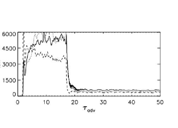
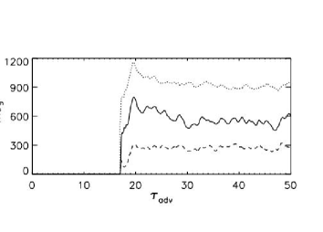
Figure 2: Time dependence of the kinetic energy and the magnetic energy. $x$-component (solid), $y$-component (dotted), $z$-component (dashed). $\Lambda=1$.

Figure 2 shows the temporal behavior of the kinetic energies $E_{\mathrm{kin}}^{x,y,z}=\int dV\rho u^{2}_{x,y,z}/2$ (left) and the magnetic energies $E_{\mathrm{mag}}^{x,y,z}=\int dV(2\mu_{0})^{-1}B^{2}_{x,y,z}$ (right) for the simulation with $\Lambda=1$. The first part of the simulation up to $t\approx 17\tau_{\mathrm{adv}}$ corresponds to thermal convection without rotation and without magnetic field. At $t\approx 17\tau_{\mathrm{adv}}$ the effects of rotation and magnetic field are added seen by a significant drop in the kinetic energies (left panel of figure 2) and a sharp increase of magnetic energies (right panel of figure 2). After a short transition phase the energy of the different components remains approximately constant for the remainder of time. A large-scale magnetic field in $x$-direction establishes during the timespan $t=17\tau_{\mathrm{adv}}...20\tau_{\mathrm{adv}}$ (see also Figure 5 below) which is associated with a remarkable amount of magnetic energy stored in the $x$-component (solid line in the right panel of figure 2).

Since the induction equation (1) for the mean magnetic field gives $\partial_{t}\left<B_{z}\right>=0$ no $\left<B_{z}\right>$ can evolve during the simulations. Therefore, the magnetic energy in the vertical field component results from the fluctuating component $B_{z}^{\prime}$. The time dependence of the energies is qualitatively similar for all runs. Major differences appear in the amount of quenching after the effects of rotation and magnetic field have abruptly been introduced.

Figure 3: Left: Quenching of turbulent velocity and (normalized) magnetic field fluctuations. Right: Ratio of the magnetic energy to the kinetic energy as a function of $\Lambda$.

The behavior of the fluctuating quantities is shown in Figure 3 where the turbulent velocity ${u_{\mathrm{rms}}}$ and the normalized turbulent magnetic field ${B}_{\mathrm{rms}}/B_{y}^{0}$ (where $B_{\mathrm{rms}}$ is defined analog to $u_{\mathrm{rms}}$) in dependence of the imposed magnetic field respective $\Lambda$ is presented. Both quantities are significantly reduced compared to a non-magnetic but rotating convective state, indicating the trend to a more laminar flow.

The ratio between the total magnetic energy and the kinetic energy is plotted in Fig. 3 (right). Equipartition is reached for $\Lambda\approx 0.6$ indicated by the dotted lines. For $\Lambda>0.6$ the magnetic energy clearly exceeds the kinetic energy. For $\Lambda=100$ the magnetic energy dominates the kinetic energy by a factor of 100.

When increasing $\Lambda$ from 0.01 to 1000 the combined effects of rotation and magnetic field lead to Rossby numbers from $7\cdot 10^{-2}$ to $1\cdot 10^{-2}$ and turbulent Mach numbers $\mathrm{Ma}={u_{\mathrm{rms}}}/c_{s}$ from $7\cdot 10^{-2}$ to $1\cdot 10^{-2}$. This is still much larger than the real Mach number in the fluid outer core which is assumed to be of the order of $10^{-7}$. Reynolds numbers, $\mathrm{Re}={u_{\mathrm{rms}}}d/\nu$, are in the range from Re=210 for $\Lambda=0.01$ and Re=32 for $\Lambda=1000$.

3.2 Patterns of flow and magnetic field

The dynamical influence of the imposed magnetic field can be seen in figure 4 where the $z$-component of the velocity near the domain faces and in a horizontal plane at $z=0.5$ is shown. The left (right) panel shows a snapshot of the developed rotating magnetoconvection for $\Lambda\approx 1$ (10). Upflows are visualized in grey whereas downflows are represented in dark tones. Compared to non-magnetic, rotating convection the magnetoconvection pattern remains nearly unchanged for $\Lambda\raisebox{-2.58334pt}{$\stackrel{{\scriptstyle{\displaystyle<}}}{{\sim}}$}1$. Many topologically not connected columnar convection cells can be seen tilted by an angle of $45^{\circ}$ with respect to the $z$-axis and become aligned with the rotation axis (Taylor-Proudman theorem).

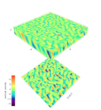
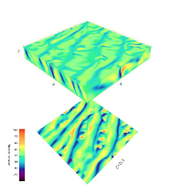
Figure 4: Vertical velocity pattern of rotating magnetoconvection for $\Lambda=1$ (left) and $\Lambda=10$ (right).

Stronger magnetic fields lead to remarkable changes in the flow pattern. Between $\Lambda=1$ and $\Lambda=4$ the quasi-regular pattern becomes more and more disintegrated and evolves towards a nearly two-dimensional flow as illustrated in the right panel of Figure 4. The convection cells are clearly elongated along the imposed magnetic field direction ($y$-direction) and show little variations of the convective velocity along the field lines. The sheetlike convection cells are again tilted inside the box and aligned with the rotation axis $\it{\Omega}$ as it is the case for the weak-field calculations. Compared to the cases of rotating convection or weak-field rotating magnetoconvection, the strong-field case is further characterized by a significant reduction of the number of convective cells. The nearly two-dimensionality of the flow can be explained from a condition similar to the Taylor-Proudman theorem for rotating spheres: For a stationary state with small deviations from the basic unperturbed state and neglecting diffusive terms it follows from the induction equation that $B_{i}\partial_{i}u_{j}=0$ i.e. motions cannot vary in the direction of the imposed magnetic field (Chandrasekhar, 1961).

3.3 Mean fields and $\alpha$-coefficients

Figure 5 shows the components of the horizontally averaged magnetic field in units of the initial field $B_{0}$ for the cases $\Lambda=0.1,1,10$. The light gray lines represent different snapshots within the averaging period indicating substantial fluctuations, and the thick dashed line gives the time average of these individual curves.

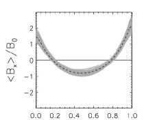
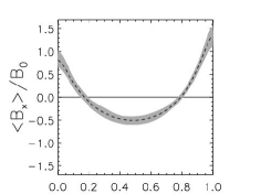
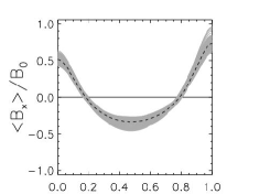
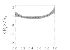
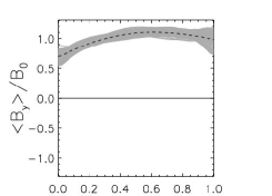
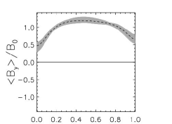
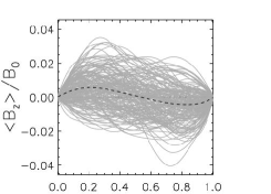
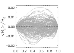
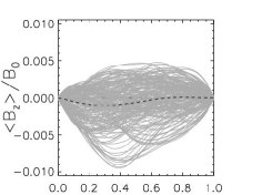
Figure 5: $z$-dependence of mean magnetic fields for $\Lambda=0.1,1,10$ (from left to right). From top to bottom: $\left<B_{x}\right>,\left<B_{y}\right>$ and $\left<B_{z}\right>$

There exists in all cases a significant magnetic field component $\left<B_{x}\right>$ close to the boundaries and in the bulk having opposite signs in that regions. This behavior strongly differs from the results reported by Ziegler (2002) for highly stratified convection where the $x$-component of the magnetic field was found negligible ($\left<B_{x}\right>\ll\left<B_{y}\right>$). This is probably due to a much lower Taylor number employed in the simulations of Ziegler (2002) and due to the initial two-layer configuration consisting of a convectively instable layer on top of a stable layer. The generation of $\left<B_{x}\right>$ at the vertical boundaries is a result of the perfect conductor boundary conditions for the magnetic field which means that no magnetic flux can cross the boundaries favoring concentration of magnetic flux at the top and at the bottom of the domain.

As expected, no significant mean magnetic field in $z$-direction establishes. For weak imposed fields local dynamo action leads to a slight amplification of $\left<B_{y}\right>$ close to the boundaries. This effect does not take place for stronger imposed fields where, in contrast, a reduction of $\left<B_{y}\right>$ occurs at the vertical boundaries.

Usually, the dynamo $\alpha$-coefficients are computed in a simplified way by

$$\mathcal{E}_{x}=\alpha_{xy}\left<B_{y}\right>,\qquad\mathcal{E}_{y}=\alpha_{yy}\left<B_{y}\right>,\qquad\mathcal{E}_{z}=\alpha_{zy}\left<B_{y}\right>.$$ (11)

This may not be justified with the mean field configuration obtained here, since the presence of a $\left<B_{x}\right>$ and the presence of gradients of the mean field components close to the vertical boundaries lead to a contribution from non-diagonal coefficients of the $\alpha$-tensor (describing the anisotropy) and from turbulent diffusivity. Their contribution cannot be easily separated without contradiction, so it seems more reasonable to regard the calculated EMF-components as the more relevant quantities. This is confirmed by calculations of Brandenburg et al. (1990) who showed that the expressions (11) together with the mean field induction equation (1) are too simple for reproducing the mean-field components as computed numerically from solving the full set of MHD-equations. However, these workers have assumed that this deviation occurs for shorter timescales whereas for longer timescales the correct time dependence of the mean-field is retained if a suitable quenching function for $\alpha$ is used. Due to the well-known theoretical background of characteristic properties for the $\alpha$-coefficients and to provide input data for a mean-field $\alpha^{2}$-dynamo model we nevertheless use relationship (11) keeping in mind that it stands for a more or less rough approximation.

In principle, with the present simulations it is possible to calculate the three coefficients $\alpha_{xy},\alpha_{yy}\mbox{ and }\alpha_{zy}$. Here, we want to concentrate on the first two coefficients $\alpha_{xy}$ and $\alpha_{yy}$. $\alpha_{xy}$ describes turbulent (radial) advection of magnetic field (pumping), whereas $\alpha_{yy}$ describes the production of magnetic field perpendicular to $\left<B_{y}\right>$ via the $\alpha$-effect and is therefore of profound interest. The vertical profile of the calculated $\alpha$-coefficients is plotted in Figure 6 for $\Lambda=0.1,1,10,100$. The top row shows $\alpha_{xy}$ and the bottom row shows $\alpha_{yy}$. Again the grey lines represent snapshots of the coefficients at different times and the dashed line in each plot represents the time-averaged $z$-profile.

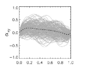
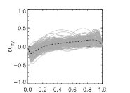
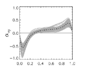
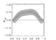
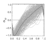
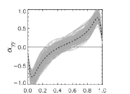
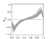
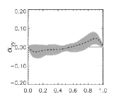
Figure 6: $z$-dependence of $\alpha_{xy}$ (top) and $\alpha_{yy}$ (bottom) for $\Lambda=0.1,1,10,100$ (from left to right) at $\theta=45^{\circ}$. Note the reduction in scale by a factor of 5 for the $\Lambda=100$ case.

We note that $\alpha_{yy}(z)$ shows a quite asymmetric behavior with respect to $z$. It is always negative in the lower part of the layer and positive in the upper part of the layer. The transition between negative and positive $\alpha$-effect occurs roughly in the middle of the box. The peaks of $\alpha_{yy}$ are remarkably broad leading to two extended zones with positive and negative $\alpha$-effect having nearly equal amplitude. Comparable solutions proportional to $\sin(2\pi z)$ from quasi-linear calculations have been found by Soward (1979). For increasing magnetic field time fluctuations in the $\alpha$-coefficients are obviously reduced which comes from the fact that the flow tends to become laminar for large $\Lambda$. The resulting vertical profiles of $\alpha_{yy}$ differ from computations with stronger stratification where the $z$-dependence is much more asymmetric. In the latter scenario the zero line is crossed in the lower half-box and the peak of the $\alpha$-coefficients is higher in the upper half-box. This leads to a non-zero $\alpha$-effect when averaged over the entire box volume (Rüdiger and Hollerbach, 2004). In contrast to this, the volume averaged $\alpha$-effect is rather small in our model.

$\alpha_{xy}(z)$ shows a drastic change in its behavior between $\Lambda=0.1$ and $\Lambda=1$. For $\Lambda=0.1$ $\alpha_{xy}$ has a broad peak located in the lower part of the layer and changes its sign close to the upper vertical boundary. For $\Lambda\geq 1$ $\alpha_{xy}$ shows a reversed $z$-dependence. This feature is correlated with the change of behavior of $\left<B_{y}\right>$ at the boundaries between $\Lambda=0.1$ and $\Lambda=1$.

Computations with a box located at $\theta=135^{\circ}$ reveal $\alpha_{xy}$ symmetric with respect to the equator but $\alpha_{yy}$ antisymmetric (see Figure 7). The resulting $\left<B\right>(z)$ closely resemble the symmetry properties of the $\alpha$-coefficients ($\left<B_{x}\right>$ antisymmetric, $\left<B_{y}\right>$ symmetric). From that it follows that the coefficient $\alpha_{xy}$ plays the role of an (negative) advection velocity ($u^{\rm esc}=-\alpha_{xy}$). The $z$-profile of $\alpha_{xy}$ shows no preferred symmetry with respect to the middle of the unstable layer, and $\alpha_{xy}$ is – independently of $\Lambda$ – predominantly positive. The escape velocity in the vertical direction is thus directed downwards for strong magnetic fields. Exactly this behavior has been obtained in a quasi-linear approximation by Kitchatinov and Rüdiger (1992) characterized as ’turbulent buoyancy’. The same result has been found in numerical simulations by Dorch and Nordlund (2001), Ossendrijver et al. (2002) and Ziegler and Rüdiger (2003). It can now be considered as a well-established phenomenon that the magnetic-induced turbulent pumping transports mean magnetic field downwards rather than upwards to the surface.

$\hskip 79.6678pt\Lambda=1\hskip 170.71652pt\Lambda=10$

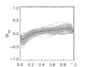
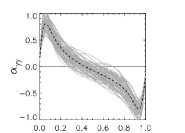
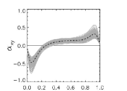
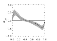
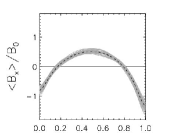
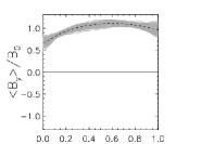
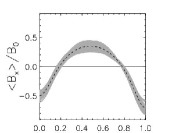
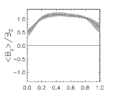
Figure 7: $z$-dependence of $\alpha_{xy}$ and $\alpha_{yy}$ (upper row) and the corresponding $\left<B_{x}\right>$ and $\left<B_{y}\right>$ (lower row) for $\Lambda=1$ and $\Lambda=10$ at $\theta=135^{\circ}$

3.4 Kinetic helicity

Figure 8 shows the $z$-profile of the kinetic helicity ${H}_{\mathrm{kin}}=\left<\mbox{\boldmath$u$}^{\prime}\cdot\nabla\times{\mbox{\boldmath$u$}^{\prime}}\right>$. The kinetic helicity is negative in the upper part of the box and positive in the lower part.

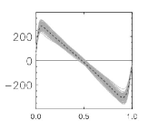
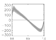
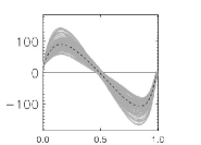
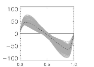
Figure 8: $z$-dependence of the kinetic helicity for $\Lambda=0.1,1,10,100$

Comparing figure 8 with the corresponding $\alpha_{yy}$-profiles from figure 6 the well-known relation between the signs of the $\alpha$-coefficient and the kinetic helicity is confirmed, i.e. $\alpha\sim-1/3\tau_{\mathrm{cor}}\left<\mbox{\boldmath$u$}^{\prime}\cdot\nabla\times{\mbox{\boldmath$u$}^{\prime}}\right>$ with a correlation time $\tau_{\mathrm{cor}}$(see e.g. Krause and Rädler, 1980). A similar relation was found by Ossendrijver et al. (2001). Increasing the strength of the imposed magnetic field the change in amplitude of the helicity is roughly in accordance with the change in amplitude of $\alpha_{yy}$. The correlation time $\tau_{\mathrm{cor}}$ roughly is of the order of $10\%$ of the turnover time $\tau_{\mathrm{adv}}$

3.5 $\alpha$-quenching

In order to estimate the quenching behavior of the $\alpha$-effect we investigate the variation of the local maximum (minimum) value of the time averaged $z$-profile $\alpha_{yy}(z)$ in dependence of the quantity $(B_{y}^{0}/B_{\mathrm{eq}})^{2}$ where $B_{y}^{0}$ denotes the initially imposed magnetic field strength and ${B}_{\mathrm{eq}}$ is the so called equipartition field which is defined by ${B}_{\mathrm{eq}}^{2}=\mu_{0}\rho{u}_{\mathrm{rms}}^{2}({B}\!\rightarrow\!0)$, i.e. $u_{\mathrm{rms}}$ is related to the non-magnetic case. In a rough approximation we have $\Lambda\approx 6.24\cdot(B_{y}^{0}/B_{\mathrm{eq}})^{2}$. The quenching curves are plotted in figure 9 where the solid (dotted) line corresponds to the maximum (minimum) of $\alpha_{yy}(z)$. The dashed line corresponds to a simple analytic quenching function of the form

$$\alpha({B})=\alpha({B}\!\rightarrow\!0)\cdot\frac{1}{1+\left(B_{y}^{0}/B_{\mathrm{eq}}\right)^{2}}.$$ (12)

A detailed analysis of the $\alpha$-quenching phenomenon for slow rotation, however, can be found in Rüdiger and Kitchatinov (1993). The corresponding expressions for $\alpha_{yy}$ is given by the dashed-dotted line in figure 9. It overestimates the suppression of $\alpha_{yy}$ so that $\alpha$-quenching is probably better described by equation (12) for our case of a fast rotator. Note that the curves associated with the maximum respective minimum of $\alpha_{yy}$ are almost identical for $(B_{y}^{0}/B_{\mathrm{eq}})^{2}\raisebox{-2.58334pt}{$\stackrel{{\scriptstyle{\displaystyle>}}}{{\sim}}$}0.2$ and the deviation is at most about $10\%$ for $(B_{y}^{0}/B_{\mathrm{eq}})^{2}\raisebox{-2.58334pt}{$\stackrel{{\scriptstyle{\displaystyle<}}}{{\sim}}$}0.2$.

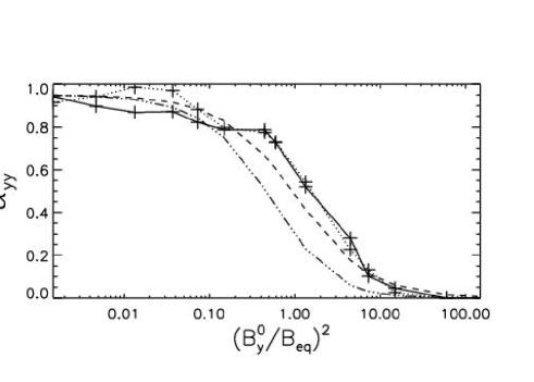
Figure 9: Quenching behavior of $\alpha_{yy}$. A value of $(B_{y}^{0}/B_{\mathrm{eq}})^{2}=1$ (equipartition value) corresponds to $\Lambda\approx 6.2$. The solid (dotted) line corresponds to the maximum (minimum) of $\alpha_{yy}(z)$, the dashed line corresponds to the analytic quenching function (12) and the dashed-dotted line represents the analytic expression derived by Rüdiger and Kitchatinov (1993).

For the dynamo number, $C_{\mathrm{\alpha}}=\alpha d/\eta$, we obtain a value of the order of $10$ for imposed fields below $(B_{y}^{0}/B_{\mathrm{eq}})^{2}\approx 1$. This value might be large enough to allow global dynamo action in the sense of $\alpha^{2}$-dynamos but this, of course, is a very crude estimation.

4 Conclusions

The main result of our computations is that the $y$-component of the EMF describing the $\alpha$-effect in the azimuthal direction is positive in the upper part of the unstable layer and negative in the lower part on the northern hemisphere. We obtained the $z$-profiles of the $\alpha$-coefficient for a wide range of imposed magnetic field strength with the amplitude of the $\alpha$-effect probably sufficient to ensure dynamo action in mean-field calculations.

The $\alpha$-effect is quenched under the influence of strong external magnetic fields but the suppression is not catastrophic, and significant quenching only sets in for magnetic fields above the equipartition value ${B_{\mathrm{eq}}}$.

Some weak points in the above model calculations should be mentioned. First, we neglected the radial dependence of the gravitational force and the effects of spherical geometry, thus, the influence of curvature effects remains unknown. Compositional convection is ignored and the adopted parameter values are still far from the realistic values for the Earth. Somewhat unphysical boundary conditions have been used by assuming the conditions of a perfect conductor for both vertical boundaries so it cannot be ruled out that the obtained profiles are profoundly affected by the vertical boundary conditions. Test calculations with rigid boundary conditions for the velocity and/or slightly different boundary conditions for the magnetic field as used e.g. by Ossendrijver et al. (2002) or Ziegler (2002) show, however, no major differences in the EMF profiles. It remains, therefore, a much-promising ansatz for future mean-field calculations of the geodynamo taking into account the special radial profile of the $\alpha$-effect as it has been obtained in the present paper.

References

- Braginsky and Roberts (1995) Braginsky, S. I., Roberts, P., 1995. Equations governing Earth’s core and the geodynamo. Geophys. Astrophys. Fluid Dynam. 79.
- Brandenburg et al. (1990) Brandenburg, A., Tuominen, I., Nordlund, A., Pulkkinen, P., Stein, R. F., Jun. 1990. 3-D simulation of turbulent cyclonic magneto-convection. A&A 232, 277–291.
- Chandrasekhar (1961) Chandrasekhar, S., 1961. Hydrodynamic and hydromagnetic stability. International Series of Monographs on Physics, Oxford: Clarendon.
- Christensen et al. (1999) Christensen, U., Olson, P., Glatzmaier, G. A., 1999. Numerical modelling of the geodynamo: a systematic parameter study. Geophysical Journal International 138, 393–409.
- Dorch and Nordlund (2001) Dorch, S. B. F., Nordlund, Å., 2001. On the transport of magnetic fields by solar-like stratified convection. A&A 365, 562–570.
- Dormy et al. (2000) Dormy, E., Valet, J. P., Courtillot, V., 2000. Numerical models of the geodynamo and observational constraints. Geochem. Geophys Geosys. 1, 62–103.
- Glatzmaier and Roberts (1996) Glatzmaier, G. A., Roberts, P. H., 1996. On the magnetic sounding of planetary interiors. Phys. Earth Planet. Inter. 98, 207–220.
- Hollerbach (1996) Hollerbach, R., 1996. On the theory of the geodynamo. Phys. Earth Planet. Inter. 98, 163–185.
- Hollerbach (2003) Hollerbach, R., 2003. The range of timescales on which the geodynamo operates. Geodynamics Series 31, 181–192.
- Hoyng et al. (2001) Hoyng, P., Ossendrijver, M. A. J. H., Schmitt, D., 2001. The geodynamo as a bistable oscillator. Geophys. Astrophys. Fluid Dynam. 94, 263.
- Kitchatinov and Rüdiger (1992) Kitchatinov, L. L., Rüdiger, G., 1992. Magnetic-field advection in inhomogeneous turbulence. A&A 260, 494–498.
- Krause and Rädler (1980) Krause, F., Rädler, K. H., 1980. Mean-field magnetohydrodynamics and dynamo theory. Oxford: Pergamon Press.
- Kuang and Bloxham (1999) Kuang, W., Bloxham, J., 1999. Numerical Modeling of Magnetohydrodynamic Convection in a Rapidly Rotating Spherical Shell: Weak and Strong Field Dynamo Action. Journal of Computational Physics 153, 51–81.
- Ossendrijver et al. (2001) Ossendrijver, M., Stix, M., Brandenburg, A., 2001. Magnetoconvection and dynamo coefficients:. Dependence of the alpha effect on rotation and magnetic field. A&A 376, 713–726.
- Ossendrijver et al. (2002) Ossendrijver, M., Stix, M., Brandenburg, A., Rüdiger, G., 2002. Magnetoconvection and dynamo coefficients. II. Field-direction dependent pumping of magnetic field. A&A 394, 735–745.
- Roberts and Glatzmaier (2000) Roberts, P. H., Glatzmaier, G. A., 2000. Geodynamo theory and simulations. Reviews of Modern Physics 72, 1081–1123.
- Rüdiger et al. (2003) Rüdiger, G., Elstner, D., Ossendrijver, M., 2003. Do spherical -dynamos oscillate? A&A 406, 15–21.
- Rüdiger and Hollerbach (2004) Rüdiger, G., Hollerbach, R., 2004. The Magnetic Universe I - Geophysical and Astrophysical Dynamo Theory. Wiley-VCH Verlag Berlin.
- Rüdiger and Kitchatinov (1993) Rüdiger, G., Kitchatinov, L. L., 1993. Alpha-effect and alpha-quenching. A&A 269, 581–588.
- Soward (1979) Soward, A. M., 1979. Convection driven dynamos. Phys. Earth Planet. Inter. 20, 134–151.
- Stefani and Gerbeth (2003) Stefani, F., Gerbeth, G., 2003. Oscillatory mean-field dynamos with a spherically symmetric, isotropic helical turbulence parameter . Physical Review E 67, 027302.
- Zhang and Schubert (2000) Zhang, K., Schubert, G., 2000. Magnetohydrodynamics in Rapidly Rotating spherical Systems. Annual Review of Fluid Mechanics 32, 409–443.
- Ziegler (1998) Ziegler, U., 1998. NIRVANA+: An adaptive mesh code for compressible MHD. Comp. Phys. Comm. 109, 111.
- Ziegler (1999) Ziegler, U., 1999. A Cartesian adaptive mesh code for compressible MHD. Comp. Phys. Comm. 116, 65.
- Ziegler (2002) Ziegler, U., 2002. Box simulations of rotating magnetoconvection. Spatiotemporal evolution. A&A 386, 331–346.
- Ziegler and Rüdiger (2003) Ziegler, U., Rüdiger, G., 2003. Box simulations of rotating magnetoconvection. Effects of penetration and turbulent pumping. A&A 401, 433–442.