Lower limits on the Hubble Constant from models of Type Ia Supernovae

By coupling observations of type Ia supernovae with results obtained from the best available numerical models we constrain the Hubble constant, independently of any external calibrators. We find an absolute lower limit of $H_{\circ}$ $>$ 50 ${\rm km\leavevmode\nobreak\ s^{-1}\leavevmode\nobreak\ Mpc^{-1}}$. In addition, we construct a Hubble diagram with UVOIR light curves of 12 type Ia supernovae located in the Hubble flow, and when adopting the most likely values (obtained from 1-D and 3-D deflagration simulations) of the amount of $\rm{}^{56}Ni$ produced in a typical event, we find values of $H_{\circ}$ $\geq$ 66$\pm$8 and $\geq$ 78$\pm$9 ${\rm km\leavevmode\nobreak\ s^{-1}\leavevmode\nobreak\ Mpc^{-1}}$, respectively. Our result may be difficult to reconcile with recent discussions in the literature as it seems that an Einstein-de Sitter universe requires $H_{\circ}$$\simeq$ 46 ${\rm km\leavevmode\nobreak\ s^{-1}\leavevmode\nobreak\ Mpc^{-1}}$in order to fit the temperature power spectrum of the cosmic microwave background and maintain the age constraints of the oldest stars.

1 Introduction

Due to their high intrinsic luminosity and apparent uniformity, type Ia supernovae (hereafter referred to as SNe Ia) have become an important distance indicator in modern cosmology. Today, they are utilized to determine the value of the Hubble constant ($H_{\circ}$) and measure the changes of the past cosmic expansion. For this reason a number of substantial observing campaigns have recently been conducted for SNe Ia at nearby redshifts (see Leibundgut 2000, for a list). As a result there is now a considerable number of events available with superb temporal and photometric coverage. However, there has been little effort made to use these high quality data sets to link observations with the physics of SNe Ia in a systematic way. The purpose of this article is to combine results obtained from theoretical models with modern data in order to constrain the value of $H_{\circ}$.

Prior attempts to couple observations with explosion models of SNe Ia in order to determine the value of $H_{\circ}$ include the pioneering investigations of Arnett et al. (1985), followed by Branch (1992), Leibundgut & Pinto (1992), Nugent et al. (1995) and Höflich & Khokhlov (1996). These works gave promising results, constraining the Hubble constant between 45 $\leq\leavevmode\nobreak\ H_{\circ}\leavevmode\nobreak\ \leq$ 105 ${\rm km\leavevmode\nobreak\ s^{-1}\leavevmode\nobreak\ Mpc^{-1}}$, and revealed that with few assumptions, SNe Ia used in such a manner provide an attractive way to measure $H_{\circ}$, while circumventing many problems associated with the extragalactic distance ladder (see Böhm-Vitense 1997; Livio et al. 1997).

Although several progenitor models for SNe Ia are discussed, the common view favors an accreting carbon oxygen (C-O) white dwarf in a binary system, which undergoes thermonuclear incineration at or near the Chandrasekhar mass (for reviews see Hillebrandt & Niemeyer 2000; Arnett 1996; Woosley & Weaver 1986). The energy released from burning to nuclear statistical equilibrium (NSE) at the density and temperatures expected in these explosions completely disrupts the C-O white dwarf, while the subsequent light curve is powered by the Comptonization or “thermalization” of $\gamma$ rays produced from the radioactive decay of ⁵⁶Ni $\rightarrow$ ⁵⁶Co $\rightarrow$ ⁵⁶Fe. The single degenerate model became favored over the double degenerate model after strong H$\alpha$ emission was observed in SN 2002ic (Hamuy et al. 2003). The H$\alpha$ emission in this SN Ia is thought to come from circumstellar material originating from the white dwarf’s evolved companion star (Hamuy et al. 2003; Nomoto et al. 2004).

Here we use bolometric light curves of SNe Ia as a means to link observations with results obtained from models of an exploding C-O white dwarf. Bolometric light curves constructed from observations provide a simple and direct route to probe the complicated explosion physics and radiation transport. As it is typically more straightforward to extract the total flux (hence luminosity) of a SN Ia from models rather than the flux for individual filters, which require complicated multi-group calculations (Leibundgut & Pinto 1992; Eastman 1997; Höflich 1997; Leibundgut 2000) bolometric light curves provide a sorely needed tool to connect observations with models. In addition, observed bolometric light curves are easily constructed from the integration of broad-band photometry, and near maximum light they reflect the fraction of $\gamma$ rays thermalized. Consequently $\sim$80% or more (Suntzeff 1996, 2003) of the thermalized flux from the $\gamma$ rays is emitted at optical and near-infrared wavelengths (3000-10000 Å), therefore what we manufacture from the observed photometry has been coined a UVOIR bolometric light curve. It must be noted that by neglecting the small amount of flux outside the UVOIR wavelength regime we introduce a systematic underestimation on the calculated values of H_∘. However, we address this systematic error when placing constraints on H_∘ (see below). The summed UVOIR flux also offers the advantage that we do not need to apply any K-corrections, which are necessary when just using individual filter passbands of SNe Ia located in the Hubble flow. Essentially, we can reduce the problem to one of energy balances where the energy inputs from the radioactive decays and the losses due to $\gamma$ ray escape can be compared to the observed wavelength-integrated flux of the SNe Ia.

In the following we utilize a set of well observed SNe Ia to demonstrate, via two methods, (see below $\S$ 4 and $\S$ 5) that –under the assumption that SNe Ia are a product of the thermonuclear disruption of a Chandrasekhar-mass C-O white dwarf– it proves to be rather difficult to obtain a value of $H_{\circ}$ $<$ 50 ${\rm km\leavevmode\nobreak\ s^{-1}\leavevmode\nobreak\ Mpc^{-1}}$. Our results, along with recent detection of the integrated Sachs-Wolfe (ISW) effect (Boughn & Crittenden 2004a, b) observed in the Wilkinson Microwave Anisotropy Probe (WMAP) data, (Bennett et al. 2003; Spergel et al. 2003) cast doubts on recent discussions in the literature (see Blanchard et al. 2003; Shanks 2004), which suggest “alternatives” to the concordance cosmological model. Spatially flat, matter-dominated Einstein-de Sitter models may produce a temperature power spectrum that can fit cosmic microwave background (CMB) observations just as accurately as the best concordance model, which sports a dark energy component. However, Einstein-de Sitter models require very low values of the Hubble constant (e.g. $H_{\circ}$ $\simeq$ 46 ${\rm km\leavevmode\nobreak\ s^{-1}\leavevmode\nobreak\ Mpc^{-1}}$) and are unable to account for the observed ISW effect.

The structure of this paper is as follows: in $\S$ 2 we briefly discuss the basic details and information that we can extract from a UVOIR/bolometric light curve. This is followed by a short discussion of the data we have compiled and the method with which we construct our UVOIR light curves. In $\S$ 3 we discuss different models of SNe Ia and the $\rm{}^{56}Ni$ yields we adopt for a typical SN Ia. We then present in $\S$ 4 a method to derive $H_{\circ}$ through the combination of observations and the theoretical $\rm{}^{56}Ni$ masses calculated in explosion models. Section 5 contains a discussion of the classical way to derive $H_{\circ}$ through the Hubble diagram of SNe Ia. Contrary to previous methods we employ here the bolometric flux. We conclude in $\S$ 6.

2 Bolometric Lightcurves of SNe Ia

2.1 UVOIR Bolometric Lightcurves

Here we provide a basic description of a typical UVOIR light curve and the physics that is thought to be driving its evolution and specific characteristics at different epochs. During maximum light the dynamical time (i.e. time since explosion) is approximately equal to the diffusion time for photons trapped within the ejecta. This causes a reduction in the opacity, which then allows a larger fraction of photons to escape the expanding ejecta (Pinto & Eastman 2001). The majority of the observable supernova flux is emitted in the optical. After maximum light an ever increasing fraction of $\gamma$ rays escape freely and no longer deposit their energy in the ejecta. They are lost in the energy balance. In addition, due to a lack of near-infrared ($JHK$-passbands) data, we neglect a small contribution of flux (no more than $\sim$5% near maximum light) in our constructed UVOIR light curves (Contardo 2001). Right after maximum light as both the $\gamma-$ray deposition rate and the temperature, hence opacity, decrease, it is believed that there is a release of ‘old’ photons, causing the observed luminosity to briefly overshoot the energy input from radioactive decay. After the release of stored energy the light curve declines in luminosity until between 20 and 40 days after maximum light, where an inflection point is seen in most events (see Suntzeff (1996) and Contardo et al. (2000)). After $\sim$60 days the bolometric light curve begins to follow a nearly linear decline of 0.026$\pm$0.002 mag/day (Contardo et al. 2000) as the energy input from radioactive decay decreases exponentially and less energy is deposited by the $\gamma$ rays. At this time the infrared contribution rises to around 10% (Contardo et al. 2000). About a year after maximum the nebula no longer traps any $\gamma$ rays and the UVOIR light curve is completely powered by positrons (Milne, The, & Leising 1999).

With UVOIR light curves and accurate distances we are able to obtain a measure of the total luminosity and, through application of Arnett’s Rule, the quantity of ⁵⁶Ni produced from burning to NSE (Arnett 1982; Arnett et al. 1985). Arnett’s Rule simply states that during the epoch of maximum light the luminosity of a SN Ia is equal to the instantaneous energy deposition rate from the radioactive decays within the expanding ejecta (see also Pinto & Eastman 2000a, b). This rule has been utilized by Suntzeff (1996), Vacca & Leibundgut (1997), Contardo et al. (2000), Strolger et al. (2002), and Candia et al. (2003) to determine the amount of ⁵⁶Ni produced in a number of SNe Ia. These efforts have revealed that the explosions of SNe Ia do indeed produce a range in the amount of ⁵⁶Ni synthesized from $\sim$0.1 $M_{\sun}$ associated with the subluminous variety of SNe Ia to $\approx\leavevmode\nobreak\$1 $M_{\sun}$ for the most luminous ones. We are now in the position to use UVOIR light curves of a fair sample of well-observed SNe Ia to probe the explosion mechanism. Hopefully in the near future it will be possible to place constraints on models as they become more sophisticated. In a subsequent paper we will provide a detailed analysis of the bolometric light curves and derived $\rm{}^{56}Ni$ masses for a large number of well observed SNe Ia.

2.2 Observational data

As mentioned above, there are a number of past (and present) dedicated monitoring programs located around the world that have assembled large collections of SNe Ia data. Programs which we have used here include: the Calán/Tololo Survey (Hamuy et al. 1995, 1996c), the Center for Astrophysics (Riess et al. 1999a; Jha 2002), and the Supernovae Optical Infrared Survey (SOIRS) (Hamuy et al. 2001).

We selected only SNe Ia located in the Hubble flow ($\geq$ 3000 km s^-1) with excellent $(U)BVRI$-band observations and that contain at least two pre-maximum observations in most photometric bands. Four of the SNe Ia compiled here include $U$-band photometry, and for those events without $U$-filter observations we added a correction (see below). At this stage, no corrections were made to account for contributions by $UV$-flux blueward of the atmospheric cutoff and near-infrared $JHK$-band photometry.

Table 1 lists all the SNe Ia (and references) we have used along with information pertaining to the amount of reddening that we have adopted for each event. Values listed for Galactic reddening were taken from the COBE dust maps of Schlegel et al. (1998), while host galaxy reddenings were procured from a variety of literature sources. To be as consistent as possible we used reddenings given in Phillips et al. (1999) for all SNe Ia that coincided with our sample. For those events not included in Phillips et al. (1999) we adopted values from the literature giving preference to those calculated via the Phillips method. The reddening for the host galaxy of SN 1999dq was taken from Riess et al. (2004).

Finally, in Table 1 we list the two observables that are employed to constrain H_∘. This includes the host galaxy recession velocity and the UVOIR bolometric flux at maximum light. Heliocentric velocities obtained from NED were converted to the CMB frame. As all SNe Ia listed in Table 1 are located in the Hubble flow, we assumed an error of 400 km s^-1 for all velocities, in order to account for (random) peculiar motions. The uncertainties listed with the bolometric fluxes account for (1) a small measurement error, which is less than 5% and (2) the uncertainties associated with estimates of host galaxy extinction.

2.3 Construction of UVOIR Lightcurves

We construct UVOIR light curves in the same manner previously adopted by Vacca & Leibundgut (1996, 1997), Contardo et al. (2000) and Contardo (2001). The reader is referred to these papers for a detailed discussion of this empirical fitting method and their previously attained results; here we briefly summarize the main points.

We attempt to fit SNe Ia photometry in a completely objective way. Data for each filter is fitted with a ten parameter function. This function consists of a Gaussian, corresponding to the peak phase on top of a linear decline for the late time decay, an exponentially rising function for the initial rise to maximum, and a second Gaussian for the secondary maximum in the $VRI$ light curves. Fitting photometry in this manner is advantageous because a continuous representation of the light curves is produced without resorting to templates that may wash out subtleties of each filtered light curve. The ten fitted parameters and several other interesting quantities can be used to explore the finer details of SNe Ia light curves (see Contardo 2001; Stritzinger 2005).

To produce a UVOIR light curve we first fit the light curve of each passband. Each magnitude is then converted to its corresponding flux at the effective wavelength and a reddening correction is applied. The flux for each filter at a given epoch is then integrated over wavelengths to get the total flux. Note, corrections are employed to account for overlaps and gaps between passbands. We also included a compensation in a manner similar to Contardo et al. (2000) for those SNe Ia that have no $U$-band photometry. Contardo et al. used a correction based on SN 1994D (Richmond et al. 1995; Patat et al. 1996; Meikle et al. 1996; Smith et al. 2000), however, this event had an unusually blue color at maximum and corrections based on it tend to overestimate the fraction of flux associated with the $U$-band photometry. We instead employed a correction derived from SN 1992A (Suntzeff 1996), which is the only well observed normal SN Ia with no host galaxy reddening. We estimate an additional 2$\%$ error is incurred on each UVOIR light curve that has our $U$-band correction.

3 $\rm{}^{56}Ni$ Yields From Explosion Models

A key ingredient for the methods presented below (see § 4 and § 5) is the amount of $\rm{}^{56}Ni$ produced in a typical SN Ia explosion. Both methods depend on the total energy radiated by the supernova to establish its distance. Contardo (2001) showed for a small sample of SNe Ia that up to a factor of 10 difference in the yield of $\rm{}^{56}Ni$ can exist between individual events. An absolute upper limit for the amount of $\rm{}^{56}Ni$ synthesized is the Chandrasekhar mass ($\sim$1.4 M_☉), when the star becomes unstable and either collapses or explodes. However, due to the presence of intermediate mass elements (IMEs) observed in spectra taken near maximum light, we know that the white dwarf is not completely burned to $\rm{}^{56}Ni$. A lower limit is provided by the subluminous events. Although only a few of these SNe Ia have been observed in detail (due to selection effects) three well observed events indicate $\sim$0.10 M_☉ of $\rm{}^{56}Ni$ is synthesized (Stritzinger 2005).

To obtain a more quantitative value we turn our attention to recent nucleosynthesis calculations performed at the Max-Planck-Institut für Astrophysik (MPA) (Travaglio et al. 2004), which are based on 3-D Eulerian hydrodynamical simulations (Reinecke et al. 2002a, b) of an exploding white dwarf, that burns via a purely turbulent deflagration flame. Based on their highest resolution 3-D simulation (i.e. model b30_3d_768), which consisted of 30 “burning” bubbles and a grid size of 768³ for 1 octant of a sphere, Travaglio et al. found the total yield of $\rm{}^{56}Ni$ to be 0.42 M_☉. However, they found that as the number of ignition spots is increased, more explosion energy is liberated, which may lead to a larger yield of $\rm{}^{56}Ni$. The number of these ignition spots is strictly dependent on the grid resolution of the simulation, which is limited by the computational facilities available. One may therefore expect a larger yield of $\rm{}^{56}Ni$ as the computational power and hence grid resolution is increased. In addition, more recent calculations that employ ignition conditions representing a foam-like structure, consisting of overlapping and individual bubbles, indicate that it may be possible to liberate a larger fraction of nuclear energy as one employs different ignition conditions (Röpke & Hillebrandt 2004).

We considered a range of results produced by other deflagration models available in the literature, in particular the phenomenological parametrized 1-D model - W7 (Nomoto, Thielemann, & Yokoi 1984). Recent nucleosynthesis calculations show that W7 synthesizes 0.59 M_☉ of $\rm{}^{56}Ni$  (Iwamoto et al. 1999). It must be noted, however, that 1-D models compared to 3-D calculations are expected to provide a less realistic representation of the physical processes that occur during thermonuclear combustions because they do not properly model the turbulent flame physics. Additionally, multidimensional effects are neglected which do have an important influence on the flame propagation. Nevertheless, W7 is a well established model that can fit the observed spectra rather well (Harkness 1991; Mazzali et al. 1995; Mazzali 2001) and has been used extensively over the last two decades to investigate SNe Ia explosions.

Despite the success of deflagration models, they are currently unable to account for the more luminous SNe Ia, and predict appreciable amounts of unburned carbon, oxygen, and IMEs leftover in the inner ashes of the ejecta, which has not yet been conclusively observed. These shortcomings were the motivation for the delayed detonation models (DDM) (Khokhlov 1991; Woosley 1990; Woosley & Weaver 1994; Höflich & Khokhlov 1996). In these models the explosions starts as a deflagration flame until a transition occurs, causing the flame to propagate supersonically thus the explosion becomes a detonation. Höflich (1995) provided a series of DDMs that range in $\rm{}^{56}Ni$ mass between $\sim$0.34 and 0.67 M_☉. His best fit model (M36) for the well observed SN 1994D produces 0.60 M_☉ of $\rm{}^{56}Ni$. The main difference to the pure deflagration models is that DDMs contain an additional free parameter that describes the local sound speed ahead of the flame. This free parameter is not physically understood but is essential to force the transition from deflagration to detonation.

Throughout the following analysis we adopt results from the highest resolution MPA simulation and the 1-D model W7. Although these two models are not meant to represent the complete range in observed luminosity for the total population of SNe Ia, they produce results that are illustrative of the majority of observed events. Both of these models are not perfect and, as results shown below indicate, the MPA model may not be representative of the more luminous events. We take the $\rm{}^{56}Ni$  masses of these two models to be representative of a fair fraction of observed SNe Ia.

As previously noted in $\S$ 1, just after maximum light the observed luminosity is expected to be larger than the radioactive luminosity, as the ejecta becomes optically thin and allows the release of stored UVOIR photons. At this epoch the photosphere rapidly recedes into the ejecta, revealing deeper layers of the progenitor allowing more spectral lines to radiate. Branch (1992) (see his Table 1) conducted a survey of the best numerical models at the time and found that the models which adequately treat the time dependent nature of the opacity near maximum light predict $\alpha$ (the ratio of energy radiated at the surface to the instantaneous energy production by the radioactive decays) to be slightly larger than unity. He concluded that $\alpha$$=$1.2$\pm$0.2 was the most applicable value and noted that the value of $\alpha$ appeared to be independent of the rise time.

The parameter $\alpha$$=$1.2$\pm$0.2 is nothing more than a correction factor that is applied to the measured luminosity derived from the model $\rm{}^{56}Ni$ masses. In the following, we take this parameter into account in our discussion of the values of H_∘ determined from the models. The $\rm{}^{56}Ni$ masses of 0.42 and 0.59 M_☉ correspond to an energy release after 19$\pm$3 days (the typical rise time of SNe Ia (Contardo et al. 2000)) of (8.40$\pm$1.26$)\times$10⁴² erg s^-1 and (1.18$\pm$0.18)$\times$10⁴³ erg s^-1, respectively. If we combine the energy production with $\alpha$$=$1.2$\pm$0.2, the luminosity is increased to 1.01$\pm$0.23$\times$10⁴³ erg s^-1 and 1.42$\pm$0.32$\times$10⁴³ erg s^-1. We note, however, that radiation transport calculations based on two MPA 3-D simulations (Blinnikov, private comm.) give the same value of $\alpha$ as calculated by Arnett’s more simple analytical models (i.e. $\alpha$$=$1).

Finally, we note that the value of $\alpha$ may vary for different SNe Ia depending on the amount and distribution of radioactive isotopes, i.e. the opacity, in the ejecta. If $\alpha$$=$1 occurs before bolometric maximum, one would expect a smaller amount of stored photons. Therefore the luminosity would tend not to overshoot the instantaneous energy deposition rate. However, if $\alpha$$=$1 occurs after bolometric maximum, the light curve should in principle, be broader and flatter.

4 H_∘ from model $\rm{}^{56}Ni$ masses

In this section we derive a first analytic expression to constrain $H_{\circ}$ directly from model $\rm{}^{56}Ni$ masses. This expression combines the UVOIR peak brightness of SNe Ia with explosion models via Arnett’s Rule (Arnett 1982).

4.1 Connecting $H_{\circ}$ and the Model Luminosities

First, we develop an analytic equation which uses a simple argument that allows one to connect $H_{\circ}$ with the amount of $\rm{}^{56}Ni$ produced in a SN Ia explosion. This relation relies on the fact that $H_{\circ}$ is defined as the ratio of the local expansion velocity to the luminosity distance, which in turn is obtained from the inverse square law for the ratio of luminosity and the observed brightness. Therefore since the luminosity of a SN Ia depends on the amount of $\rm{}^{56}Ni$, we can use the explosion models as our guide to the absolute luminosity. Combining this with both the measured brightness and recession velocity (or redshift) of any particular event, we can derive a value for $H_{\circ}$. The first expression to constrain $H_{\circ}$ therefore combines three elements: (1) Hubble’s law of local cosmic expansion, (2) the distance luminosity relation, and (3) Arnett’s Rule.

We combine Hubble’s law, which is defined by

$$H_{\circ}=\frac{cz}{D_{L}}$$ (1)

with the distance luminosity relation given by

$$D_{L}=\left(\frac{L}{4\pi F}\right)^{\frac{1}{2}}\;,$$ (2)

where $F$ corresponds to the UVOIR flux obtained from the bolometric light curves, $L$ is the luminosity of a fiducial SN Ia, and $D_{L}$ is the luminosity distance. We obtain

$$H_{\circ}=cz\left(\frac{4\pi F}{L}\right)^{\frac{1}{2}}\;.$$ (3)

At maximum light the luminosity produced by the radioactive $\rm{}^{56}Ni$  can be expressed as

$$L_{max}=\alpha E_{{\rm Ni}}(t_{R})\;,$$ (4)

where $E_{{\rm Ni}}$ is the energy input from the decay of $\rm{}^{56}Ni$, evaluated at the time of bolometric maximum (rise time $t_{R}$), and $\alpha$ accounts for any deviations from Arnett’s Rule (where $\alpha$$=$1). An expression for $E_{{\rm Ni}}$ can be found in Nadyozhin (1994)

$$E_{{\rm Ni}}(t_{R})=\frac{\lambda_{{\rm Ni}}\lambda_{{\rm Co}}}{\lambda_{{\rm Ni}}-\lambda_{{\rm Co}}}\cdot\bigg{\{}\left[Q_{{\rm Ni}}\left(\frac{\lambda_{{\rm Ni}}}{\lambda_{{\rm Co}}}-1\right)-Q_{{\rm Co}}\right]\bigg{.}\\[5.69054pt] \bigg{.}\cdot e^{-\lambda_{{\rm Ni}}t}+Q_{{\rm Co}}e^{-\lambda_{{\rm Co}}t}\bigg{\}}M_{{\rm Ni}}=\epsilon(t_{R})M_{{\rm Ni}}\;,$$ (5)

where $\lambda_{{\rm Ni}}$ and $\lambda_{{\rm Co}}$ are e-folding decay times of 8.8 and 111.3 days for ⁵⁶Ni and ⁵⁶Co, respectively, and $Q_{{\rm Ni}}$ and $Q_{{\rm Co}}$ correspond to the mean energy released per decay of 1.75 and 3.73 MeV. For 1 $M_{\sun}$ of $\rm{}^{56}Ni$, equation (5) turns into

$$E_{{\rm Ni}}(1\leavevmode\nobreak\ M_{\sun})=6.45\times 10^{43}e^{-t_{R}/8.8}+1.45\times 10^{43}e^{-t_{R}/111.3}\;.$$ (6)

Riess et al. (1999b) found, for a normal SN Ia (e.g. $\Delta m_{15}(B)$$=$1.1 mag) with a peak magnitude $M_{V}$ $=$ $-$19.45, a rise time to $B$ maximum of $\sim$19.5 days. Contardo et al. (2000) found the bolometric rise time to be within one day of the $B$-band for nearly all SNe Ia in their sample. Throughout this work we assume a bolometric rise time of 19$\pm$3 days. The adopted uncertainty should be adequate to account for intrinsic differences between the rise times of different SNe Ia. Using this rise time and assuming $\alpha$$=$1.0 (Arnett’s Rule) we can combine equations (4) and (6) and obtain the simple relation that gives for 1 M_☉ of $\rm{}^{56}Ni$  a total luminosity at maximum light of

$${\rm L_{max}}(1\leavevmode\nobreak\ M_{\sun})\leavevmode\nobreak\ =\leavevmode\nobreak\ (2.0\pm 0.3)\leavevmode\nobreak\ \times\leavevmode\nobreak\ 10^{43}\leavevmode\nobreak\ {\rm erg\leavevmode\nobreak\ s^{-1}\leavevmode\nobreak\ M^{-1}_{\sun}}\;,$$ (7)

where the error corresponds to the 3 day uncertainty in the adopted bolometric rise time.

Substituting equation (4) into equation (3) we can relate the luminosity to the mass of $\rm{}^{56}Ni$ via $E_{{\rm Ni}}$ (equation 5), and then if we include the factors that directly equate the luminosity with the $\rm{}^{56}Ni$ mass, we obtain our final relation to calculate the Hubble constant

$$H_{\circ}=cz\left(\frac{4\pi F_{max}^{bol}}{L_{max}}\right)^{\frac{1}{2}}\leavevmode\nobreak\ =\leavevmode\nobreak\ \leavevmode\nobreak\ cz\left(\frac{4\pi F_{max}^{bol}}{\alpha E_{\rm Ni}(t_{R})}\right)^{\frac{1}{2}}=cz\left(\frac{4\pi F_{max}^{bol}}{\alpha\epsilon(t_{R})M_{\rm Ni}}\right)^{\frac{1}{2}}\;.$$ (8)

With equation (8) only two observables – the bolometric flux ($F_{\rm max}^{bol}$) at maximum and the redshift ($z$) – are required to determine the value of $H_{\circ}$.

Uncertainties come from the rise time, which determines the the peak luminosity, the uncertainty in $\alpha$, which depends on the radiation escape from the explosion, and of course the amount of $\rm{}^{56}Ni$ synthesized in the explosion. Finally we note that our $\rm{}^{56}Ni$ mass is “error free” in the sense that the adopted value(s) for this parameter (hence fiducial luminosities) are completely model dependent.

We now have an analytic form for H_∘ which is directly connected to the $\rm{}^{56}Ni$ produced in the explosion. The other parameters have to do with the radiation transport: the ratio of energy release to energy input and the time between explosion and maximum luminosity.

4.2 Results

In Fig. 1 we present results obtained using equation (8) for all SNe Ia listed in Table 1. For every supernova we show the derived H_∘, assuming that its observed brightness would correspond to a given nickel mass (in steps of 0.1 M_☉). The inverse square-root dependence of H_∘ on the nickel mass is clearly visible. The ‘1-$\sigma$’ error bars that accompany each point account for a recession velocity error of 400 km s^-1, an error associated with the reddening correction, a measurement error of the flux ($\leq$ 5%), a 3 day error for the assumed bolometric rise time, and a 2% error for those events that have a $U$-band correction. Note that the most dominant error is the uncertainty associated with the redshift due to peculiar velocities.

It is evident from this figure that for a given mass of $\rm{}^{56}Ni$ there exists a range of possible values of $H_{\circ}$. This is what we expect owing to the fact that there are known intrinsic differences between SNe Ia. Hence, if we (erroneously) assume a single $\rm{}^{56}Ni$ mass for all observed SNe Ia, we obtain a range of H_∘ values as in Fig. 1.

Two SNe Ia (SN 1992bo and SN 1993H) are clearly situated below the rest of the objects and are both known to be red events with $\Delta$$m_{15}(B)=$1.69 (Hamuy et al. 1996c). Both also show evidence of weak Ti features in their spectra (Phillips, private comm.). Because the models we have adopted in this work were designed for normal SNe Ia and these two events are subluminous in nature, we exclude them in the following discussion; however, they are included in the Hubble diagram (see § 5). Given the prediction of an explosion model, we can now read off the preferred value of the Hubble constant. Naïvely, one would like to take the mean of the distribution of the supernovae for a given $\rm{}^{56}Ni$ mass and derive a Hubble constant. However, the natural scatter of $\rm{}^{56}Ni$ (Contardo et al. 2000; Bowers et al. 1997; Cappellaro et al. 1997) prevents us from doing this because only one value is correct for a given event. The best we can do now is to derive a lower limit for H_∘ by associating the nickel masses with the faintest supernovae and hence obtain an underestimate of the Hubble constant.

By choosing a $\rm{}^{56}Ni$ mass of 1 M_☉ and associating it with faint SNe Ia we clearly reach a lower limit for $H_{\circ}$. Note that the highest $\rm{}^{56}Ni$ mass derived from a SN Ia with a Cepheid distance is 0.84 M_☉ (Strolger et al. 2002). The solid horizontal line in Fig. 1 indicates that evidently more than 1 M_☉ of $\rm{}^{56}Ni$ must be produced in a normal SNe Ia explosion in order to obtain $H_{\circ}$ $<$ 50 ${\rm km\leavevmode\nobreak\ s^{-1}\leavevmode\nobreak\ Mpc^{-1}}$. Note that the two dotted vertical lines indicate our adopted $\rm{}^{56}Ni$ masses with $\alpha$$=$1.0. For both cases an H_∘ of more than 50 km s^-1 Mpc^-1 is favored. Only the two faint SNe Ia fall well below this value.

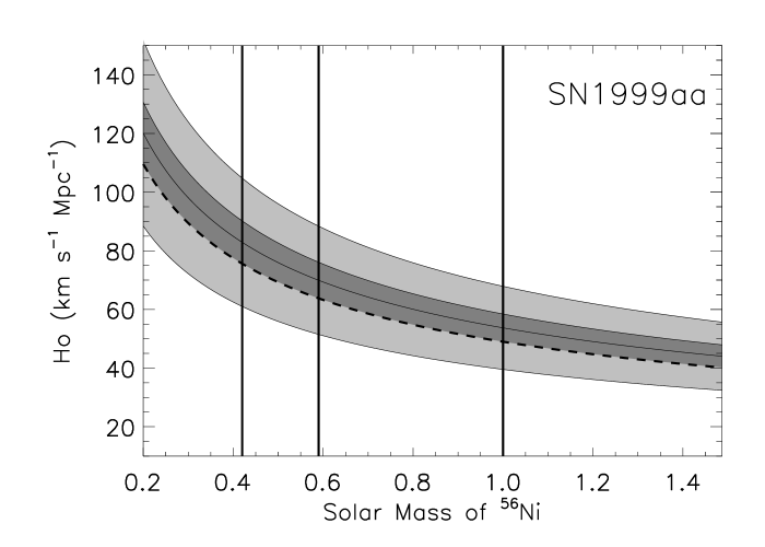
Figure 2: To highlight the absolute lower limit we derive on H_∘ we plot results obtained with SN 1999aa (the least luminous of our 10 normal SNe Ia) with 1-$\sigma$ (dark shading) and 3-$\sigma$ (light shading) confidence levels. Vertical solid lines indicate both the adopted $\rm{}^{56}Ni$ masses and the 1 M_☉ upper limit expected from an exploding C-O white dwarf. The dashed line illustrates the effect if $\alpha$ is increased by 20% (i.e. $\alpha$$=$1.2).

To obtain an absolute lower limit on $H_{\circ}$, we present in Fig. 2 the least luminous normal event in our sample – SN 1999aa – with 1-$\sigma$ and 3-$\sigma$ confidence levels. This SN Ia produces values of $H_{\circ}$ that are 9% below the mean determined from all 10 normal events. For our adopted $\rm{}^{56}Ni$ masses with $\alpha$$=$1 we obtain a lower limit on $H_{\circ}$ with SN 1999aa (3-$\sigma$ away from the calculated values) to be $\geq$ 40 ${\rm km\leavevmode\nobreak\ s^{-1}\leavevmode\nobreak\ Mpc^{-1}}$. The dashed line in Fig. 2 illustrates the effect of increasing $\alpha$ by 20%. We see that this gives us an additional systematic uncertainty that would decrease $H_{\circ}$ by 9%. The change incurred on the Hubble constant lies directly on top of the quoted lower 1$\sigma$ confidence level. Finally, we note from equation (8) that by neglecting $\sim$10% of the flux emitted outside of the optical, we systematically underestimate H_∘ by 5%.

We find that with white dwarfs as progenitors of SNe Ia it is very difficult to obtain a value of $H_{\circ}$ $<$ 50 ${\rm km\leavevmode\nobreak\ s^{-1}\leavevmode\nobreak\ Mpc^{-1}}$. With 1 M_☉ of $\rm{}^{56}Ni$, one could expect $H_{\circ}$ $\sim$60 ${\rm km\leavevmode\nobreak\ s^{-1}\leavevmode\nobreak\ Mpc^{-1}}$. Observations and models for the most luminous events indicate that no more than 1 M_☉ of $\rm{}^{56}Ni$ is produced. With our adopted $\rm{}^{56}Ni$ masses (0.42 M_☉ $<$ $\rm{}^{56}Ni$ $<$ 0.59 M_☉) we find from the 1-$\sigma$ error bars in Fig. 2 the Hubble constant to be constrain between 70$\pm$6 $\leq$ H_∘ $\leq$ 83$\pm$7 ${\rm km\leavevmode\nobreak\ s^{-1}\leavevmode\nobreak\ Mpc^{-1}}$.

The problem can, of course, also be inverted to derive a possible range of $\rm{}^{56}Ni$ mass given a value of H_∘. This will be interesting to constrain the $\rm{}^{56}Ni$ mass for models, should H_∘ be known to high accuracy. For $H_{\circ}$ $\approx\leavevmode\nobreak\$70 ${\rm km\leavevmode\nobreak\ s^{-1}\leavevmode\nobreak\ Mpc^{-1}}$we find from Fig. 1 a range in the amount of $\rm{}^{56}Ni$ produced in a SNe Ia explosion to be 0.5 M${}_{\sun}<$ $\rm{}^{56}Ni$ $<1.0$ M_☉.

5 H_∘ through the Hubble diagram of SNe Ia

With this method we determine $H_{\circ}$ from the Hubble diagram in a manner similar to what has been previously presented by Tammann & Leibundgut (1990) and Leibundgut & Pinto (1992) (see also Sandage & Tammann 1993; Hamuy et al. 1996c; Phillips et al. 1999; Parodi et al. 2000, for similar applications). We note that this method is similar to the previous method, however, here $H_{\circ}$ is calculated in a more traditional manner. An analytic expression to constrain $H_{\circ}$ from our Hubble diagram is trivial to derive from the distance luminosity relation. Solving equation (2) for $F_{max}^{bol}$ and then taking the logarithm of both sides, we obtain

$$\log(F_{max}^{bol})=\log\left(\frac{L_{max}}{4\pi D_{L}^{2}}\right)\;.$$ (9)

Substituting $cz/H_{\circ}$ for $D_{L}$ and rewriting the right hand side of equation (9) we obtain

$$\log(F_{max}^{bol})=-2\log(cz)+\log(L_{max})-\log(4\pi)+2\log(H_{\circ})\;.$$ (10)

There is a linear relation between $\log(F_{max}^{bol})$ and $\log(cz)$ as can be seen in Fig. 3. A linear regression to the data yields a slope of $2.01\pm 0.25$, which is fully consistent with the expected slope of 2 for a linear local expansion derived in equation (10). From Fig. 3 it is also obvious that the two faint objects are outliers. If they are ignored, the fit sharpens up to a slope of $1.97\pm 0.10$. With a fixed slope to this linear expansion value of $2$ we derive the y-intercept, which corresponds to

$$b=-\log(L_{max})+\log(4\pi)-2\log(H_{\circ})\;.$$ (11)

Solving equation (11) for $H_{\circ}$, we arrive at our final expression for the Hubble constant

$$H_{\circ}=\left(\frac{4\pi}{10^{b}L_{max}}\right)^{\frac{1}{2}}\;.$$ (12)

The Hubble constant is now simply calculated by plugging in the y-intercept, b, derived from the linear regression of the Hubble diagram and a fiducial luminosity defined by our adopted models.

5.1 Results

In Fig. 3 we present our Hubble diagram containing all SNe Ia listed in Table 1. Error bars for all events account for both a redshift uncertainty of 400 km s^-1 and the uncertainties associated with host galaxy reddening. A weighted least-squares fit to the Hubble diagram (for all 12 SNe Ia), with a fixed slope of $2$, yields $b$ $=$3.292$\pm$0.047. Plugging this into equation (12) along with our adopted $\rm{}^{56}Ni$ masses of 0.42 M_☉ and 0.59 M_☉ we find H_∘ to be $\geq$ 85$\pm$7 and $\geq$ 72$\pm$6 ${\rm km\leavevmode\nobreak\ s^{-1}\leavevmode\nobreak\ Mpc^{-1}}$(1-$\sigma$ error) respectively. Accounting for $\alpha$$=$1.2$\pm$0.2 we obtain lower values of the Hubble constant to be H_∘ $\geq$ 78$\pm$9 and $\geq$ 66$\pm$8 ${\rm km\leavevmode\nobreak\ s^{-1}\leavevmode\nobreak\ Mpc^{-1}}$, respectively.

As an upper limit in the amount of $\rm{}^{56}Ni$ synthesized in the most luminous SNe Ia explosion is expected to be $\approx\leavevmode\nobreak\$1 M_☉, we can use the corresponding luminosity as a guide to obtain a lower limit on the Hubble constant through the Hubble diagram. Thus, for 1 M_☉ of $\rm{}^{56}Ni$ and $\alpha$$=$1 we obtain a value of H_∘ $\geq$ 55$\pm$5 ${\rm km\leavevmode\nobreak\ s^{-1}\leavevmode\nobreak\ Mpc^{-1}}$. As in the previous method, we are underestimating H_∘ by $\sim$5%, due to flux outside the optical window.

6 Discussion

Under the main assumptions: (1) that the progenitors of SNe Ia are C-O white dwarfs that explode at or near the Chandrasekhar mass, and (2) that the amount of $\rm{}^{56}Ni$ synthesized to first order determines the peak luminosity, we are able to use results obtained from state-of-the-art numerical simulations of explosion models to uniquely define the bolometric peak luminosity, and in concert with photometric observations constrain H_∘. The attractiveness of this approach stems from the ability to bypass assumptions that are typically made when one attempts to determine H_∘, i.e. the extragalactic distance ladder and its accumulation of error from rung to rung. We stress that our fitting method does not add any corrections to the data. In other words we do not normalize the flux to any decline rate relation (e.g. $\Delta$$m_{15}$ (Phillips et al. 1999), MLCS (Riess et al. 1996) or stretch (Perlmutter et al. 1997)).

Uncertainties that marginally affect (in decreasing order of importance) our results include: the abundances of peak Fe group metals – stable and radioactive – produced in the explosion models, the redshift peculiar velocities of each SN Ia, the total absorption, the assumed rise time to bolometric maximum, the exact nature of $\alpha$, which may slightly vary from SN to SN depending on the exact nature of the opacity and ionization structure of the expanding ejecta, and the amount of flux that we neglect outside of the optical window.

It is still unclear what parameters effect the amount of $\rm{}^{56}Ni$ produced in a SN Ia explosion. Obvious candidates are the initial conditions prior to explosion. These include the metallicity of the C-O white dwarf, the central density and the ignition mechanism. If there is a considerable fraction of alpha elements such as ²²Ne within the progenitor one would expect more stable isotopes such as ⁵⁸Ni and ^54,56Fe to be produced from burning to NSE, thus reducing the $\rm{}^{56}Ni$ yield (e.g. Brachwitz et al. 2000). A higher central density on the other hand would lead to a more robust explosion and hence an increased amount of $\rm{}^{56}Ni$. As discussed earlier the explosion mechanism is still uncertain and different deflagration and detonation scenarios produce different amounts of peak Fe group elements. Nevertheless with a larger $\rm{}^{56}Ni$ mass we obtain smaller values of H_∘. Errors attributed to the adopted recession velocity and reddenings produce scatter in our Hubble diagram but have very little effect on our calculations of H_∘ via equations (8) or (12). The $\pm$3 day departure from our adopted rise has no more than a 10% effect on our calculations. A change in $\alpha$ by $\pm$20% can affect H_∘ by 9%. Finally, we reiterate from equation (8) that by neglecting $\sim$10% of the flux emitted outside of the optical, we are underestimating H_∘ by at least 5% or correspondingly more if more flux is unaccounted in our method.

In $\S$ 5.1 we determined a rather high value (85 ${\rm km\leavevmode\nobreak\ s^{-1}\leavevmode\nobreak\ Mpc^{-1}}$) for the Hubble constant when using results from the MPA model. This indicates that the amount of $\rm{}^{56}Ni$ produced in these 3-D deflagration simulations currently are on the low side. And indeed a large sample of SNe Ia show that the average distribution of $\rm{}^{56}Ni$ mass is slightly higher ($\sim$ 0.6 M_☉) (Stritzinger 2005). This suggests that their models may need more fine tuning in order to produce a larger amount of $\rm{}^{56}Ni$, and hence match observations more accurately.

There have been many attempts since Kowal (1968) presented his Hubble diagram to exploit SNe Ia to determine H_∘. We refer the reader to Branch (1998) for a detailed review of previous works that attempt to calculate H_∘ based on SNe Ia. He concluded, from methods based on physical considerations similar to the methods presented in this work and methods which utilize SNe Ia that have been independently calibrated by Cepheids, a range in the Hubble constant of 54 $\leq$ H_∘ $\leq$ 67 ${\rm km\leavevmode\nobreak\ s^{-1}\leavevmode\nobreak\ Mpc^{-1}}$, with a “consensus” on H_∘ $=$ 60$\pm$10 ${\rm km\leavevmode\nobreak\ s^{-1}\leavevmode\nobreak\ Mpc^{-1}}$. More recent investigations of Suntzeff et al. (1999) and Jha (2002) give values of H_∘ $=$ 64 ${\rm km\leavevmode\nobreak\ s^{-1}\leavevmode\nobreak\ Mpc^{-1}}$. Finally, (Freedman et al. 2001; Spergel et al. 2003; Altavilla et al. 2004) have all measured slightly larger values of H_∘ $\approx\leavevmode\nobreak\$70 ${\rm km\leavevmode\nobreak\ s^{-1}\leavevmode\nobreak\ Mpc^{-1}}$with 10% accuracy.

Another method independent of the extragalactic distance ladder which combines X-ray imaging of galactic clusters with the Sunyaev-Zel’dovich effect (SZE) has been recently used to place limits on H_∘ (Myers et al. 1997; Mason et al. 2001; Jones et al. 2003; Reese et al. 2002). These works have provided the detailed study of 41 clusters giving distances which yield an averaged value of H_∘ $\approx\leavevmode\nobreak\$61$\pm$3 ${\rm km\leavevmode\nobreak\ s^{-1}\leavevmode\nobreak\ Mpc^{-1}}$(for a review see Reese 2003).

We find from both methods presented here that the Hubble constant must be $>$ 50 ${\rm km\leavevmode\nobreak\ s^{-1}\leavevmode\nobreak\ Mpc^{-1}}$in order to be compatible with current supernova models. In addition, we stress that this lower limit is based on the assumption that 1 M_☉ is an upper limit on the amount of $\rm{}^{56}Ni$ produced in a SN Ia explosion, and not from our adopted models. This result, along with other methods to measure H_∘ using SNe Ia calibrated with Cepheids, SZE/X-ray distances and evidence of the ISW effect, strongly suggest that we do not live in a matter dominated universe without some form of cosmological constant or similar agent.

Table 1: Well-observed SNe Ia in the Hubble Flow

SN	Filters	Ref.	E(B-V)${}_{gal}^{a}$	E(B-V)host	vCMB b	F${}_{max}^{bol}$
					(km s-1)	(erg s-1 cm-2)
SN1992bc	$BVRI$	1	0.022	0.000	5870	(1.565$\pm$0.124)$\times 10^{-11}$
SN1992bo	$BVRI$	1	0.027	0.000	5151	(9.106$\pm$0.967)$\times 10^{-12}$
SN1993H	$BVRI$	1	0.060	0.050	7112	(4.640$\pm$0.613)$\times 10^{-12}$
SN1995E	$BVRI$	2	0.027	0.740	3478	(5.726$\pm$0.622)$\times 10^{-11}$
SN1995ac	$BVRI$	2	0.042	0.080	14651	(3.425$\pm$0.477)$\times 10^{-12}$
SN1995bd	$BVRI$	2	0.495	0.150	4266	(2.542$\pm$0.521)$\times 10^{-11}$
SN1996bo	$BVRI$	2	0.078	0.280	4857	(2.382$\pm$0.237)$\times 10^{-11}$
SN1999aa	$UBVRI$	3, 4, 5	0.040	0.000	4546	(2.333$\pm$0.446)$\times 10^{-11}$
SN1999aw	$BVRI$	5, 6	0.032	0.000	11754	(3.525$\pm$0.700)$\times 10^{-12}$
SN1999dq	$UBVRI$	3	0.024	0.139	4029	(3.871$\pm$0.730)$\times 10^{-11}$
SN1999ee	$UBVRI$	7	0.020	0.280	3169	(5.781$\pm$0.881)$\times 10^{-11}$
SN1999gp	$UBVRI$	3, 8	0.056	0.070	7783	(9.270$\pm$1.082)$\times 10^{-12}$

References. — (1) - Hamuy et al. 1996c, (2) - Riess et al. 1999a, (3) - Jha 2002, (4) - Krisciunas et al. 2000, (5) - Regnault 2000, (6) - Strolger et al. 2002, (7) - Stritzinger et al. 2002, (8) - Krisciunas et al. 2001

Figure 1: Hubble constant as a function of $\rm{}^{56}Ni$ mass for 12 SNe Ia in the Hubble flow for $\alpha$$=$1. Error bars represent all uncertainties discussed in section 4.1. The dotted lines indicate the two $\rm{}^{56}Ni$ masses from our adopted models. The solid vertical line indicates an upper limit on the production of $\rm{}^{56}Ni$ expected from the thermonuclear explosion of a C-O white dwarf, and the solid horizontal line corresponds to the lower limit we derive for H_∘.

Figure 3: Hubble diagram of 12 SNe Ia in the Hubble flow. The negative logarithm of the UVOIR flux at maximum light is plotted against the logarithm of the recession velocity in the CMB frame. Error bars account for a peculiar velocity of 400 km s^-1 and uncertainties associated with host galaxy reddening.