Structures in a class of magnetized scale-free discs

Abstract

We construct analytically stationary global configurations for both aligned and logarithmic spiral coplanar magnetohydrodynamic (MHD) perturbations in an axisymmetric background MHD disc with a power-law surface mass density $\Sigma_{0}\propto r^{-\alpha}$, a coplanar azimuthal magnetic field $B_{0}\propto r^{-\gamma}$, a consistent self-gravity and a power-law rotation curve $v_{0}\propto r^{-\beta}$ where $v_{0}$ is the linear azimuthal gas rotation speed. The barotropic equation of state $\Pi\propto\Sigma^{n}$ is adopted for both MHD background equilibrium and coplanar MHD perturbations where $\Pi$ is the vertically integrated pressure and $n$ is the barotropic index. For a scale-free background MHD equilibrium, a relation exists among $\alpha$, $\beta$, $\gamma$ and $n$ such that only one parameter (e.g., $\beta$) is independent. For a linear axisymmetric stability analysis, we provide global criteria in various parameter regimes. For nonaxisymmetric aligned and logarithmic spiral cases, two branches of perturbation modes (i.e., fast and slow MHD density waves) can be derived once $\beta$ is specified. To complement the magnetized singular isothermal disc (MSID) analysis of Lou, we extend the analysis to a wider range of $-1/4<\beta<1/2$. As an example of illustration, we discuss specifically the $\beta=1/4$ case when the background magnetic field is force-free. Angular momentum conservation for coplanar MHD perturbations and other relevant aspects of our approach are discussed.

1 Introduction

Magnetic fields are ubiquitous in diverse astrophysical settings on various scales ranging from proto-stellar discs, young stellar objects (YSOs), microquasars, quasars, galaxies and grandiose astrophysical jets to clusters of galaxies. In some cases, magnetic fields are relatively weak so that dynamical processes are almost unaffected by their presence. However, there do exist numerous cases where magnetic fields are necessary and important for both dynamics and diagnostics, especially in spiral galaxies and accretion disc systems (e.g., Sofue et al. 1986; Beck et al. 1996; Balbus & Hawley 1998; Tagger & Pellat 1999; Widrow 2002). In general, it is challenging to model magnetic fields realistically because of their complexities (Sofue et al. 1986; Kronberg 1994; Caunt & Tagger 2001; Widrow 2002). In the problems involving protostar formation and disc galaxies, Shu & Li (1997) presumed the so-called ‘isopedic’ magnetic field configuration where the mass-to-magnetic flux ratio in a razor thin disc remains constant. Using a singular isothermal disc (SID) model (Mestel 1963) that is isopedically magnetized, Shu et al. (2000) studied stationary coplanar perturbations and proposed that these global modes are bifurcations to either secularly or dynamically unstable configurations. Along a separate yet complementary line, Lou (2002) studied an azimuthally magnetized singular isothermal disc (MSID) and derived two different global stationary magnetohydrodynamic (MHD) perturbation modes. Based on the MSID model, Lou (2002) explored the manifestation of interlaced optical and magnetic field spiral arms in the outer portion of a disc with a nearly flat rotation curve such as the case of the nearby spiral galaxy NGC 6946 (Beck & Hoernes 1996; Fan & Lou 1996; Lou & Fan 1998a, 2002; Frick et al. 2000, 2001; Lou et al. 2002).

In contexts of spiral galaxies, it is natural and important to consider a composite disc system consisting of gravitationally coupled gaseous and stellar discs. This is because various physical processes on different scales occur in the gaseous disc yet large-scale gas dynamics and environment are significantly affected by large-scale structures in the stellar disc (Lou & Fan 1998b). To construct global coplanar perturbation structures in a systematic manner, we started with a composite SID system of two fluid discs without magnetic field (Lou & Shen 2003) to generalize the work of Shu et al. (2000) for a single SID. In terms of the global axisymmetric stability for such a composite SID system, we provided a more straightforward $D-$criterion (Shen & Lou 2003) in contrast to the axisymmetric stability criteria of Elmegreen (1995) and Jog (1996). To be more general than a background SID profile, we recently constructed global stationary perturbation patterns in a composite system of two fluid scale-free discs without magnetic field (Shen & Lou 2004a, b) to further generalize the work of Syer & Tremaine (1996). With proper adaptations, these global stationary perturbation solutions may be utilized to model large-scale structures spiral galaxies.

While a scale-free disc has no characteristic scales, one may impose boundary conditions to describe a modified scale-free disc, e.g., by cutting a central hole in a disc (e.g., Zang 1976; Evans & Read 1998a, b). With such boundary conditions, discrete eigenfunctions for perturbations may be constructed as growing normal modes. On the other hand, by specifying a phase relation for a postulated reflection of spiral waves from the origin $r=0$, Goodman & Evans (1999) could also define discrete normal modes even for an unmodified gaseous SID. Shu et al. (2000) speculated that the swing amplification process (e.g., Goldreich & Lynden-Bell 1965; Julian & Toomre 1966; Toomre 1977; Fan & Lou 1997) across corotation allows a continuum of normal modes (Lynden-Bell & Lemos 1993) while proper ‘boundary conditions’ may select from this continuum a discrete spectrum of unstable normal modes; they also suggested that zero-frequency (stationary) disturbances do signal the onset of instability.

On the basis of the work of Shu et al. (2000) for a single isopedically magnetized SID and of Lou & Shen (2003) for a composite SID system without magnetic field, Lou & Wu (2004) analyzed coplanar MHD perturbation structures in a composite SID system with one of the disc being isopedically magnetized (Shu & Li 1997). As X-ray emitting hot gases can freely flow along open magnetic field lines anchored at the gaseous disc, global stationary solutions constructed by Lou & Wu (2004) set an important preliminary stage for modelling spiral galactic MHD winds. In particular, if activities of star formation, starbursts and supernovae etc. are mainly responsible for producing X-ray emitting hot gases streaming out of the galactic plane from both sides, we would expect stronger winds from the circumnuclear starburst region (e.g. Lou et al. 2001) and along spiral arms than those winds from the remainder of the galactic disc plane.

Both SID and MSID models offer valuable physical insight for disc dynamics and belong to a wider family of scale-free discs (Syer & Tremaine 1996) where physical variables in the axisymmetric background equilibrium scale as powers of radius $r$ (e.g., the rotation curve $\propto r^{-\beta}$). It turns out that coplanar perturbations in such scale-free discs in a proper range of $\beta$ can be treated globally and analytically (Lemos et al. 1991; Syer & Tremaine 1996) without invoking the usual WKBJ or tight-winding approximation to solve the Poisson equation for density wave perturbations (Lin & Shu 1964; Binney & Tremaine 1987; Bertin & Lin 1996). In other words, it becomes feasible to include azimuthal magnetic fields in a scale-free disc and to construct global coplanar MHD perturbation configurations that are stationary in an inertial frame of reference. Such analytical solutions, still idealized and limited, are making important further steps and are extremely valuable for bench-marking numerical codes and for initializing numerical MHD simulations.

For an azimuthally magnetized scale-free disc with an infinitesimal thickness, the axisymmetric background equilibrium without radial flow is characterized by following features: a surface mass density $\Sigma_{0}\propto r^{-\alpha}$, a rotation curve $v_{0}\propto r^{-\beta}$, an azimuthal magnetic field $B_{0}\propto r^{-\gamma}$ and a barotropic equation of state $\Pi=K\Sigma^{n}$ where $\Pi$ is the vertically integrated gas pressure with constant $K>0$ for a warm disc and $n>0$ as the barotropic index. To maintain a radial force balance at all radii, there exists an explicit relationship among $\alpha$, $\beta$, $\gamma$ and $n$ such that only one parameter is independent. As will be seen in Section 2, it is convenient to use $\beta$ as this independent parameter (Syer & Tremaine 1996; Shen & Lou 2004b). In order to satisfy relevant constraints, the prescribed range of $\beta$ turns out to be $-1/4<\beta<1/2$ that includes the previous special case of $\beta=0$ (i.e., the MSID case) studied by Lou (2002), Lou & Zou (2004a) and Lou & Wu (2004). In Section 2, we introduce coplanar MHD perturbations and present the linearized perturbation equations. We construct and analyze global stationary aligned and logarithmic spiral perturbation configurations in Section 3 and as an example of illustration, we discuss specifically the case of $\beta=1/4$ with the background azimuthal magnetic field being force-free. In Section 4, we derive phase relationships between perturbation enhancements of surface mass density and magnetic field for both aligned and logarithmic spiral cases, and discuss the problem of angular momentum conservation. Finally, we summarize our results in Section 5. For the convenience of reference, relevant technical details are collected in the Appendices.

2 Formulation of the Problem

In the magnetofluid approximation, the disc is taken to be razor-thin (i.e., we use vertically integrated magnetofluid equations and neglect vertical derivatives of physical variables) and large-scale stationary aligned and spiral coplanar disturbances develop in a background MHD rotational equilibrium of axisymmetry (Syer & Tremaine 1996; Lou 2002; Lou & Zou 2004a; Lou & Wu 2004). The background magnetic field is taken to be azimuthal to avoid the magnetic field winding dilemma (Lou & Fan 1998a). For the sake of simplicity at this stage, non-ideal effects such as viscosity, resistivity and thermal diffusion etc. are ignored for large-scale perturbations.

2.1 Basic Coplanar MHD Equations in a Cylindrical Disc Geometry

Using cylindrical coordinates $(r,\theta,z)$, we have the following two-dimensional nonlinear MHD equations for a razor-thin disc geometry: the mass conservation equation

$$\frac{\partial\Sigma}{\partial t}+\frac{1}{r}\frac{\partial(r\Sigma u)}{\partial r}+\frac{1}{r^{2}}\frac{\partial(\Sigma j)}{\partial\theta}=0\ ,$$ (1)

where $\Sigma$ is the surface mass density, $u$ is the radial bulk flow velocity, $j\equiv rv$ is the specific angular momentum in the vertical $\hat{z}$-direction and $v$ is the azimuthal linear velocity; the radial component of the momentum equation

$$\begin{split}\frac{\partial u}{\partial t}+u\frac{\partial u}{\partial r}+\frac{j}{r^{2}}\frac{\partial u}{\partial\theta}-\frac{j^{2}}{r^{3}}=-\frac{1}{\Sigma}\frac{\partial\Pi}{\partial r}-\frac{\partial\phi_{T}}{\partial r}-\frac{1}{\Sigma}\int\frac{dzB_{\theta}}{4\pi r}\bigg{[}\frac{\partial(rB_{\theta})}{\partial r}-\frac{\partial B_{r}}{\partial\theta}\bigg{]}\ ,\end{split}$$ (2)

where $\Pi$ is the vertically integrated gas pressure (sometimes referred to as two-dimensional pressure), $\phi_{T}$ is the total gravitational potential including that of an axisymmetric dark matter halo in contexts of disc galaxies, and $B_{\theta}$ and $B_{r}$ are the azimuthal and radial components of the coplanar magnetic field $\vec{B}$, respectively; the azimuthal component of the momentum equation

$$\begin{split}\frac{\partial j}{\partial t}+u\frac{\partial j}{\partial r}+\frac{j}{r^{2}}\frac{\partial j}{\partial\theta}=-\frac{1}{\Sigma}\frac{\partial\Pi}{\partial\theta}-\frac{\partial\phi_{T}}{\partial\theta}+\frac{1}{\Sigma}\int\frac{dzB_{r}}{4\pi}\bigg{[}\frac{\partial(rB_{\theta})}{\partial r}-\frac{\partial B_{r}}{\partial\theta}\bigg{]}\ ;\end{split}$$ (3)

the Poisson integral equation

$$F\phi_{T}=-G\oint d\psi\int_{0}^{\infty}\frac{\Sigma(r^{\prime},\psi,t)r^{\prime}dr^{\prime}}{[r^{\prime 2}+r^{2}-2r^{\prime}r\cos(\psi-\theta)]^{1/2}}\ ,$$ (4)

where $F\equiv\phi/\phi_{T}$ is defined as the ratio of the potential arising from the disc to that arising from the entire system including a massive dark matter halo that is presumed not to respond to coplanar perturbations in the disc plane (Syer & Tremaine 1996; Shu & Li 1997; Shu et al. 2000; Lou & Shen 2003; Shen & Lou 2004a, b; Lou & Zou 2004a) with $F=1$ for a full disc and $0<F<1$ for partial discs; the divergence-free condition of magnetic field $\vec{B}\equiv(B_{r},\ B_{\theta},\ 0)$

$$\frac{\partial(rB_{r})}{\partial r}+\frac{\partial B_{\theta}}{\partial\theta}=0\ ;$$ (5)

the radial component of the magnetic induction equation

$$\frac{\partial B_{r}}{\partial t}=\frac{1}{r}\frac{\partial}{\partial\theta}(uB_{\theta}-vB_{r})\ ;$$ (6)

the azimuthal component of the magnetic field induction equation

$$\frac{\partial B_{\theta}}{\partial t}=-\frac{\partial}{\partial r}(uB_{\theta}-vB_{r})\ ;$$ (7)

and the barotropic equation of state

$$\Pi=K\Sigma^{n}\ ,$$ (8)

where constants $K>0$ and $n>0$. Among the three equations (5), (6) and (7), we can freely choose two independent ones. By barotropic equation of state (8), the sound speed $a$ is defined by

$$a^{2}\equiv\frac{d\Pi_{0}}{d\Sigma_{0}}=nK\Sigma_{0}^{n-1}\ ,$$ (9)

where subscript $0$ indicates the background equilibrium. An isothermal sound speed corresponds to a barotropic index $n=1$.

2.2 Properties of an Axisymmetric Equilibrium

We now proceed to derive properties of an axisymmetric rotational MHD equilibrium characterized by physical variables associated with a subscript $0$. In our notations, such a background equilibrium has the following power-law scalings: surface mass density of $\Sigma_{0}\propto r^{-\alpha}$, a radial velocity profile $u_{0}=0$ and $j_{0}\equiv rv_{0}\propto r^{1-\beta}$, a purely azimuthal magnetic field with $B_{r}^{0}=0$ and $B_{\theta}^{0}\equiv B_{0}\propto r^{-\gamma}$. Substitutions of these power-law scalings into equations $(\ref{MassConv})-(\ref{soundspeed})$ lead to the following condition for the radial force balance, namely

$$v_{0}^{2}+\alpha a^{2}-(1-\gamma)C_{A}^{2}=r\frac{d\phi_{T}^{0}}{dr}\ ,$$ (10)

where the Alfvén speed $C_{A}$ in a thin disc is defined by

$$C_{A}^{2}\equiv\frac{1}{4\pi\Sigma_{0}}\int B_{0}^{2}dz$$ (11)

and the Poisson integral gives

$$F\phi_{T}^{0}=-2\pi Gr\Sigma_{0}{\cal P}_{0}(\alpha)\ ,$$ (12)

with the numerical factor ${\cal P}_{0}(\alpha)$ explicitly defined by

$${\cal P}_{0}(\alpha)\equiv\frac{\Gamma(-\alpha/2+1)\Gamma(\alpha/2-1/2)}{2\Gamma(-\alpha/2+3/2)\Gamma(\alpha/2)}\$$ (13)

and $\Gamma(...)$ being the standard gamma function. This expression (13) can also be included in a more general form of ${\cal P}_{m}(\beta)$ as in expression (42) derived later with the limiting result of $2\beta{\cal P}_{0}(\beta)\rightarrow 1$ as $\beta\rightarrow 0$.

To satisfy the radial force balance equation (10) at all radii (i.e., scale-free) would necessarily require

$$2\beta=\alpha(n-1)=2\gamma-\alpha=\alpha-1\ ,$$ (14)

which immediately leads to the explicit expressions of indices $\alpha$, $\gamma$ and $n$ all in terms of $\beta$

$$\alpha=1+2\beta\ ,\qquad\gamma=\frac{(1+4\beta)}{2}\ ,\qquad n=\frac{(1+4\beta)}{(1+2\beta)}\ .$$ (15)

In this formulation, $\phi_{T}^{0}$ remains finite only if $1<\alpha<2$ which implies $0<\beta<1/2$. For the total gravity force arising from the equilibrium surface mass densities to be finite, a larger $\beta-$range $\beta\in(-1/2,1/2)$ is allowed. The $\beta-$range is also constrained by $-1/4<\beta<1/2$ where the first inequality is required for $n>0$ and the second inequality is imposed such that the central point mass will not diverge. By these considerations, the plausible range of $\beta$ falls in $(-1/4,1/2)$ (see Syer & Tremaine 1996 and Shen & Lou 2004a, b).

According to equations (10) and (15), we can explicitly write all physical variables of the background equilibrium state in power-law scalings of $r$ in terms of parameter $\beta$, namely

$$\begin{split}&\Sigma_{0}=\frac{FA^{2}[1+D^{2}-(1-4\beta)q^{2}/(2+4\beta)]}{2\pi G(2\beta{\cal P}_{0})r^{1+2\beta}}\ ,\ \ \qquad a^{2}=\frac{A^{2}}{(1+2\beta)r^{2\beta}}\ ,\ \ \qquad C_{A}^{2}\equiv q^{2}a^{2}=\frac{q^{2}A^{2}}{(1+2\beta)r^{2\beta}}\ ,\\ &v_{0}=\frac{AD}{r^{\beta}}\ ,\ \ \qquad j_{0}\equiv rv_{0}=\frac{AD}{r^{\beta-1}}\ ,\ \ \qquad\Omega\equiv\frac{j_{0}}{r^{2}}=\frac{AD}{r^{1+\beta}}\ ,\ \ \qquad\kappa\equiv[(2\Omega/r)d(r^{2}\Omega)/dr]^{1/2}=[2(1-\beta)]^{1/2}\Omega\ .\end{split}$$ (16)

By introducing a reference radius $R$, the constant $A$ is actually related to a scaled sound speed $a(1+2\beta)^{1/2}R^{\beta}$, the constant $D=v_{0}/[a(1+2\beta)^{1/2}]$ is a scaled rotational Mach number, the constant $q$ is the ratio of the Alfvén speed $C_{A}$ to the sound speed $a$, $\Omega$ and $\kappa$ are the equilibrium angular speed and the epicyclic frequency, respectively (Lou 2002; Shen & Lou 2004a, b). The first expression of equation (16) puts an upper limit on the magnetic field strength, namely, $1+D^{2}-(1-4\beta)q^{2}/(2+4\beta)>0$. Alternatively, once a magnetic field parameter $q^{2}$ is chosen, the scaled rotational Mach number $D$ must meet the following physical requirement

$$D^{2}>\frac{(1-4\beta)q^{2}}{(2+4\beta)}-1\$$ (17)

for a positive equilibrium surface mass density $\Sigma_{0}$. Note that for $1/4\leq\beta<1/2$, inequality (17) is automatically satisfied without actually restricting $q^{2}$ and the relevant physical requirement is simply $D^{2}>0$. Not all stationary solutions of $D^{2}$ can satisfy condition (17). This then implies limits on allowed magnetic field strength for a known background rotational MHD equilibrium.

It is also important to note that for the axisymmetric background rotational MHD equilibrium under consideration, the magnetic force arising from the azimuthal magnetic field is radially inward when $-1/4<\beta<1/4$, radially outward when $1/4<\beta<1/2$ and is zero when $\beta=1/4$ [i.e., the azimuthal magnetic field is force-free (Lou & Fan 1998a) and the equilibrium density distribution reduces to that of the single unmagnetized disc case (Lemos et al. 1991; Syer & Tremaine 1996)]. These different possibilities can be physically understood in terms of the competition between the magnetic pressure and tension forces. In order to see this more specifically for the background, we can write $-(4\pi\Sigma r)^{-1}\int dzB_{0}\partial(rB_{0})/\partial r=-{\Sigma}^{-1}[(\partial/\partial r)\int B_{0}^{2}dz/(8\pi)+\int B_{0}^{2}dz/(4\pi r)]$ referring to equation (2). The first term in the square brackets stands for the magnetic pressure force and the second term stands for the magnetic tension force for a purely azimuthal magnetic field $B_{0}(r)$ in the cylindrical geometry. As $B_{0}$ scales $r^{-\gamma}$, we have $(\partial/\partial r)\int B_{0}^{2}dz/(8\pi)+\int B_{0}^{2}dz/(4\pi r)=(-\gamma+1)\int B_{0}^{2}dz/(4\pi r)$. Therefore for $0<\gamma<1$ or equivalently $-1/4<\beta<1/4$, the magnetic tension force dominates and the total magnetic force is radially inward; for $1<\gamma<3/2$ or equivalently $1/4<\beta<1/2$, the magnetic pressure force dominates and the total magnetic force is radially outward. The two magnetic forces balance each other for $\gamma=1$ (or $\beta=1/4$).

2.3 Coplanar MHD Perturbations in the Disc Plane

On the basis of the full MHD equations $(\ref{MassConv})-(\ref{AzimuMInduct})$, we readily derive the linearized coplanar MHD perturbation equations as

$$\frac{\partial\Sigma_{1}}{\partial t}+\frac{1}{r}\frac{\partial(r\Sigma_{0}u_{1})}{\partial r}+\Omega\frac{\partial\Sigma_{1}}{\partial\theta}+\frac{\Sigma_{0}}{r^{2}}\frac{\partial j_{1}}{\partial\theta}=0\ ,$$ (18)

$$\begin{split}\frac{\partial u_{1}}{\partial t}+\Omega\frac{\partial u_{1}}{\partial\theta}-\frac{2\Omega j_{1}}{r}=-\frac{\partial}{\partial r}\bigg{(}\frac{a^{2}\Sigma_{1}}{\Sigma_{0}}+\phi_{1}\bigg{)}+\frac{(1-4\beta)C_{A}^{2}\Sigma_{1}}{2\Sigma_{0}r}-\frac{1}{\Sigma_{0}}\int\frac{dzB_{0}}{4\pi r}\bigg{[}\frac{\partial(rb_{\theta})}{\partial r}-\frac{\partial b_{r}}{\partial\theta}\bigg{]}-\frac{1}{\Sigma_{0}}\int\frac{dzb_{\theta}}{4\pi r}\frac{\partial(rB_{0})}{\partial r}\ ,\end{split}$$ (19)

$$\begin{split}\frac{\partial j_{1}}{\partial t}+\frac{r\kappa^{2}}{2\Omega}u_{1}+\Omega\frac{\partial j_{1}}{\partial\theta}=-\frac{\partial}{\partial\theta}\bigg{(}\frac{a^{2}\Sigma_{1}}{\Sigma_{0}}+\phi_{1}\bigg{)}+\frac{1}{\Sigma_{0}}\int\frac{dzb_{r}}{4\pi}\frac{\partial(rB_{0})}{\partial r}\ ,\end{split}$$ (20)

$$\phi_{1}=-G\oint d\psi\int_{0}^{\infty}\frac{\Sigma_{1}(r^{\prime},\psi,t)\ r^{\prime}dr^{\prime}}{[r^{\prime 2}+r^{2}-2r^{\prime}r\cos(\psi-\theta)]^{1/2}},$$ (21)

$$\frac{\partial(rb_{r})}{\partial r}+\frac{\partial b_{\theta}}{\partial\theta}=0\ ,$$ (22)

$$\frac{\partial b_{r}}{\partial t}=\frac{1}{r}\frac{\partial}{\partial\theta}(u_{1}B_{0}-r\Omega b_{r})\ ,$$ (23)

$$\frac{\partial b_{\theta}}{\partial t}=-\frac{\partial}{\partial r}(u_{1}B_{0}-r\Omega b_{r})\ ,$$ (24)

where we use subscript $1$ to denote associations with small disturbances in physical variables and $\vec{b}\equiv(b_{r},b_{\theta},0)$ stands for the coplanar magnetic field perturbation. As the background rotational MHD equilibrium is stationary and axisymmetric, these perturbed physical variables can be decomposed in terms of Fourier harmonics with the periodic dependence $\exp(i\omega t-im\theta)$ where $\omega$ is the angular frequency and $m$ is an integer for azimuthal variations. More specifically, we write

$$\begin{split}&\Sigma_{1}=S(r)\exp(\hbox{i}\omega t-\hbox{i}m\theta)\ ,\quad\qquad u_{1}=U(r)\exp(\hbox{i}\omega t-\hbox{i}m\theta),\quad\qquad j_{1}=J(r)\exp(\hbox{i}\omega t-\hbox{i}m\theta)\ ,\\ &\phi_{1}=V(r)\exp(\hbox{i}\omega t-\hbox{i}m\theta)\ ,\quad\qquad b_{r}=R(r)\exp(\hbox{i}\omega t-\hbox{i}m\theta)\ ,\quad\qquad b_{\theta}=Z(r)\exp(\hbox{i}\omega t-\hbox{i}m\theta)\ ,\end{split}$$ (25)

where $S(r)$, $U(r)$, $J(r)$, $V(r)$, $R(r)$ and $Z(r)$ are all radial variations of the corresponding perturbed physical variables and can be complex in general for possible radial oscillations. Without loss of generality, we take $m\geq 0$ in our analysis.

With Fourier decomposition (25), it is then straightforward to cast coplanar MHD perturbation equations $(\ref{Perturb1})-(\ref{Perturb7})$ into the following forms of

$$\hbox{i}(\omega-m\Omega)S+\frac{1}{r}\frac{\partial}{\partial r}(r\Sigma_{0}U)-\frac{\hbox{i}m\Sigma_{0}}{r^{2}}J=0\ ,$$ (26)

$$\begin{split}\hbox{i}(\omega-m\Omega)U-\frac{2\Omega J}{r}=-\frac{\partial\Phi}{\partial r}+\frac{(1-4\beta)C_{A}^{2}S}{2\Sigma_{0}r}-\frac{1}{\Sigma_{0}}\int\frac{dzZ}{4\pi r}\frac{\partial(rB_{0})}{\partial r}-\frac{1}{\Sigma_{0}}\int\frac{dzB_{0}}{4\pi r}\bigg{[}\frac{\partial(rZ)}{\partial r}+\hbox{i}mR\bigg{]}\ ,\end{split}$$ (27)

where $\Phi\equiv a^{2}S/\Sigma_{0}+V$ is a short-hand notation, and

$$\hbox{i}(\omega-m\Omega)J+\frac{r\kappa^{2}}{2\Omega}U=\hbox{i}m\Phi+\frac{1}{\Sigma_{0}}\int\frac{dzR}{4\pi}\frac{\partial(rB_{0})}{\partial r}\ ,$$ (28)

$$V(r)=-G\oint d\psi\int_{0}^{\infty}\frac{S(r^{\prime})\cos(m\psi)r^{\prime}dr^{\prime}}{(r^{\prime 2}+r^{2}-2rr^{\prime}\cos\psi)^{1/2}}\ ,$$ (29)

$$\frac{\partial(rR)}{\partial r}-\hbox{i}mZ=0\ ,$$ (30)

$$\hbox{i}(\omega-m\Omega)R+\frac{\hbox{i}mB_{0}}{r}U=0\ ,$$ (31)

$$\hbox{i}\omega Z=\frac{\partial}{\partial r}(r\Omega R)-\frac{\partial}{\partial r}(B_{0}U)\ ,$$ (32)

where equation (32) can be derived by combining equations (30) and (31).

We now rearrange the time-dependent coplanar MHD perturbation equations by taking $m\geq 1$ from equations (26)$-$(32); and the special case of $m=0$ will be analyzed in details at the end of this subsection.

From equations (30) and (31), we readily obtain

$$\begin{split}Z=-\frac{\hbox{i}}{m}\frac{\partial(rR)}{\partial r}\ ,\qquad\qquad R=-\frac{mB_{0}U}{r(\omega-m\Omega)}\ .\end{split}$$ (33)

A substitution of equation (33) into the radial and azimuthal components of the momentum equation (27) and (28) yields

$$\begin{split}\hbox{i}(\omega-m\Omega)U-\frac{2\Omega J}{r}=-\frac{\partial\Phi}{\partial r}+\frac{(1-4\beta)C_{A}^{2}S}{2\Sigma_{0}r}-\hbox{i}C_{A}^{2}\bigg{[}\frac{\partial^{2}}{\partial r^{2}}+\frac{1-12\beta}{2r}\frac{\partial}{\partial r}+\frac{2\beta(1+4\beta)-m^{2}}{r^{2}}\bigg{]}\bigg{(}\frac{U}{\omega-m\Omega}\bigg{)}\ ,\end{split}$$ (34)

and

$$\hbox{i}(\omega-m\Omega)J+\frac{r\kappa^{2}}{2\Omega}U=\hbox{i}m\Phi-\frac{mC_{A}^{2}(1-4\beta)}{2r}\bigg{(}\frac{U}{\omega-m\Omega}\bigg{)}\ ,$$ (35)

respectively.

In order to construct global solutions without the WKBJ approximation, we are mainly interested in stationary configurations with zero pattern speed $\omega/m=0$, also referred to as neutral $\omega=0$ modes (e.g., Syer & Tremaine 1996; Shu et al. 2000; Lou 2002; Shen & Lou 2004a, b; Lou & Zou 2004a). By setting $\omega=0$ and taking $m\geq 1$, equations (26), (33), (34) and (35) can be readily reduced to

$$m\Omega S+\frac{1}{r}\frac{\partial}{\partial r}(r\Sigma_{0}\hbox{i}U)+\frac{m\Sigma_{0}}{r^{2}}J=0\ ,$$ (36)

$$Z=-\frac{\partial}{\partial r}\bigg{(}\frac{B_{0}\hbox{i}U}{m\Omega}\bigg{)}\ ,\qquad\qquad\qquad R=\frac{B_{0}U}{r\Omega}\ ,$$ (37)

$$\begin{split}m\Omega\hbox{i}U+\frac{2\Omega J}{r}=\frac{\partial\Phi}{\partial r}-\frac{(1-4\beta)C_{A}^{2}S}{2\Sigma_{0}r}-\frac{C_{A}^{2}}{m}\bigg{[}\frac{\partial^{2}}{\partial r^{2}}+\frac{1-12\beta}{2r}\frac{\partial}{\partial r}+\frac{2\beta(1+4\beta)-m^{2}}{r^{2}}\bigg{]}\frac{\hbox{i}U}{\Omega}\ ,\end{split}$$ (38)

$$m\Omega J+\frac{r\kappa^{2}}{2\Omega}\hbox{i}U=-m\Phi+\frac{C_{A}^{2}(1-4\beta)}{2r}\frac{\hbox{i}U}{\Omega}\ .$$ (39)

Equations (36) through (39) together with equation (29) are the basic MHD perturbation equations for constructing stationary non-axisymmetric $m\geq 1$ configurations of both aligned and unaligned logarithmic spiral cases. Note that aligned and spiral stationary global solutions both involve propagations of fast and slow MHD density waves (Lou 2002).

We next present the basic coplanar MHD perturbation equations for stationary axisymmetric $m=0$ configurations with or without radial propagations. Starting from equations (26), (31), (32), (34) and (35) by setting $m=0$ and $\omega\neq 0$, we obtain

$$\begin{split}&\omega S=\frac{1}{r}\frac{\partial}{\partial r}(r\Sigma_{0}\hbox{i}U)\ ,\\ &\omega^{2}\hbox{i}U-\frac{2\omega\Omega J}{r}=-\omega\frac{\partial\Phi}{\partial r}+\omega\frac{(1-4\beta)C_{A}^{2}S}{2\Sigma_{0}r}-C_{A}^{2}\bigg{[}\frac{\partial^{2}}{\partial r^{2}}+\frac{1-12\beta}{2r}\frac{\partial}{\partial r}+\frac{2\beta(1+4\beta)}{r^{2}}\bigg{]}\hbox{i}U\ ,\\ &\omega J=\frac{r\kappa^{2}}{2\Omega}\hbox{i}U\ ,\\ &R=0\ ,\qquad\qquad\omega Z=\frac{\partial}{\partial r}(B_{0}\hbox{i}U)\ .\end{split}$$ (40)

This set of equations is applicable as we proceed to investigate stationary axisymmetric coplanar MHD perturbations (Lou & Zou 2004a, b). For coplanar hydrodynamic perturbations or coplanar MHD perturbations in an isopedically magnetized SID (Shu et al. 2000), there is no essential difference for changing the order of limiting procedure for $m=0$ and $\omega\rightarrow 0$. However, for MSID with a coplanar azimuthal background magnetic field, the results would be different by changing the order of limiting procedure for $m=0$ and $\omega\rightarrow 0$ (Lou 2002; Lou & Fan 2002; Lou & Zou 2004a).

3 Stationary Aligned and Logarithmic Spiral Configurations

To solve the Poisson equation connecting the perturbed surface mass density and the perturbed gravitational potential, we may consistently assume disturbances to carry proper scale-free forms (Lynden-Bell & Lemos 1993) for aligned and logarithmic spiral perturbations. For aligned perturbations, $S(r)$ contains only an amplitude variation in $r$ of perturbed surface mass density and does not involve phase variation in $r$ so that the maximum density perturbations at different radii line up in the azimuth. For spiral perturbations in comparison, in addition to an amplitude variation in $r$, $S(r)$ also involves a phase variation in $r$ such that a spiral pattern emerges.

3.1 Aligned Global Coplanar MHD Configurations

For aligned global coplanar MHD perturbations, we select those perturbations that carry the same power-law variation in $r$ of the background equilibrium, namely

$$S=\sigma r^{-1-2\beta}\ ,\qquad\qquad V=-2\pi GrS{\cal P}_{m}(\beta)\ ,$$ (41)

where $\sigma$ is a small constant coefficient and the numerical factor ${\cal P}_{m}(\beta)$ is given explicitly by

$${\cal P}_{m}(\beta)=\frac{\Gamma(m/2-\beta+1/2)\Gamma(m/2+\beta)}{2\Gamma(m/2-\beta+1)\Gamma(m/2+\beta+1/2)}\ ,$$ (42)

where $-m/2<\beta<(m+1)/2$ (Qian 1992; Syer & Tremaine 1996; Shen & Lou 2004a, b). In the limit of $\beta\rightarrow 0$, we simply have ${\cal P}_{m}=1/m$ consistent with earlier results on SIDs and MSIDs (Shu et al. 2000; Lou 2002; Lou & Shen 2003; Lou & Zou 2004a; Lou & Wu 2004). In fact, a more general class of self-consistent potential-density pairs satisfying the Poisson integral (29) is also available; see footnote 3 in Shen & Lou (2004b).

3.1.1 Aligned $m=0$ Case

For aligned neutral modes of axisymmetry ($m=0$), we can start from equation (40) by setting $\omega=0$; this implies $U=R=0$ and gives no constraints on $Z$. As $S\propto r^{-1-2\beta}$, the scale-free condition requires $Z\propto r^{-\gamma}$ with $\gamma=1/2+2\beta$ and $J\propto r^{1-\beta}$. It turns out that such stationary coplanar MHD perturbations are simply alternative states for the axisymmetric background equilibrium with a proper rescaling factor (Shu et al. 2000; Lou 2002). As this is somewhat trivial, we now turn our attention mainly to cases of non-axisymmetric $m\geq 1$ stationary aligned coplanar MHD perturbations.

3.1.2 Aligned $m\geq 1$ Cases

For the potential-density pair $S\propto r^{-1-2\beta}$ and $V=-2\pi G{\cal P}_{m}rS$, we have $U\propto r^{-\beta}$ and $J\propto r^{1-\beta}$ according to equations $(\ref{stationary1})-(\ref{stationary4})$. It then follows that

$$\begin{split}&m\Omega S-\frac{3\beta}{r}\Sigma_{0}\hbox{i}U+\frac{m\Sigma_{0}}{r^{2}}J=0\ ,\\ &m\Omega\hbox{i}U+\frac{2\Omega}{r}J=\frac{2\beta a^{2}}{r\Sigma_{0}}\bigg{(}\frac{r\Sigma_{0}}{a^{2}}2\pi G{\cal P}_{m}-1\bigg{)}S-\frac{(1-4\beta)C_{A}^{2}}{2\Sigma_{0}r}S-\frac{C_{A}^{2}[(1-4\beta)^{2}-2m^{2}]}{2m\Omega r^{2}}\hbox{i}U\ ,\\ &m\Omega J+r(1-\beta)\Omega\hbox{i}U=\frac{ma^{2}}{r\Sigma_{0}}\bigg{(}\frac{r\Sigma_{0}}{a^{2}}2\pi G{\cal P}_{m}-1\bigg{)}rS+\frac{C_{A}^{2}(1-4\beta)}{2\Omega r}\hbox{i}U\ ,\\ &Z=-\bigg{(}\frac{1}{2}-2\beta\bigg{)}\frac{B_{0}\hbox{i}U}{m\Omega r}\ ,\qquad\qquad\qquad R=\frac{B_{0}U}{\Omega r}\ .\end{split}$$ (43)

Rearranging the first three equations of (43), we obtain a set of three algebraic equations, namely

$$\begin{split}a_{1}S+b_{1}\hbox{i}U+c_{1}J=0\ ,\qquad\qquad a_{2}S+b_{2}\hbox{i}U+c_{2}J=0\ ,\qquad\qquad a_{3}S+b_{3}\hbox{i}U+c_{3}J=0\ ,\end{split}$$ (44)

where coefficients $a_{i}$, $b_{i}$, $c_{i}$ ($i=1,2,3$) are explicitly defined by

$$\begin{split}&a_{1}\equiv m\Omega\ ,\qquad\qquad b_{1}\equiv-\frac{3\beta\Sigma_{0}}{r}\ ,\qquad\qquad c_{1}\equiv\frac{m\Sigma_{0}}{r^{2}}\ ,\\ &a_{2}\equiv\frac{(1-4\beta)C_{A}^{2}}{2\Sigma_{0}r}-2\beta\bigg{[}2\pi G{\cal P}_{m}(\beta)-\frac{a^{2}}{\Sigma_{0}r}\bigg{]}\ ,\quad\qquad b_{2}\equiv m\Omega+\frac{[(1-4\beta)^{2}-2m^{2}]C_{A}^{2}}{2m\Omega r^{2}}\ ,\quad\qquad c_{2}\equiv\frac{2\Omega}{r}\ ,\\ &a_{3}\equiv-mr\bigg{[}2\pi G{\cal P}_{m}(\beta)-\frac{a^{2}}{\Sigma_{0}r}\bigg{]}\ ,\qquad\qquad b_{3}\equiv r(1-\beta)\Omega-\frac{(1-4\beta)C_{A}^{2}}{2\Omega r}\ ,\qquad\qquad c_{3}\equiv m\Omega\ .\end{split}$$ (45)

For nontrivial solutions of $\{S\ ,\ \hbox{i}U\ ,\ J\}$, the determinant of algebraic equations (44) must vanish, namely

$$a_{1}-\frac{b_{1}(a_{2}c_{3}-a_{3}c_{2})}{(b_{2}c_{3}-b_{3}c_{2})}+\frac{c_{1}(a_{2}b_{3}-a_{3}b_{2})}{(b_{2}c_{3}-b_{3}c_{2})}=0\ .$$ (46)

Using coefficient definitions (45) in condition (46), we obtain a more informative form of stationary dispersion relation

$$\begin{split}\frac{a^{2}-2\pi G{\cal P}_{m}\Sigma_{0}r-\Omega^{2}r^{2}}{(1/2-2\beta)C_{A}^{2}-(1+2\beta)\Omega^{2}r^{2}}=&\frac{\Omega^{2}r^{2}[6\beta a^{2}+(2-2\beta)\Omega^{2}r^{2}-12\beta\pi G{\cal P}_{m}\Sigma_{0}r-(1-4\beta)C_{A}^{2}]}{[m^{2}\Omega^{2}r^{2}-C_{A}^{2}(m^{2}-1/2-8\beta^{2}+4\beta)][(1+2\beta)\Omega^{2}r^{2}-C_{A}^{2}(1/2-2\beta)]}\ \\ &\qquad\qquad\qquad-\frac{4\beta a^{2}-8\beta\pi G{\cal P}_{m}\Sigma_{0}r+(1-4\beta)C_{A}^{2}}{2[m^{2}\Omega^{2}r^{2}-C_{A}^{2}(m^{2}-1/2-8\beta^{2}+4\beta)]}\ .\end{split}$$ (47)

Note that equation (47) takes a simpler form in the limit of $\beta\rightarrow 0$ (i.e., a flat rotation curve of a SID) and reduces to equation (3.1.9) of Lou (2002) as expected.

By using background MHD equilibrium variables (16) in condition (47), we obtain the stationary dispersion relation for global aligned $m\geq 1$ coplanar MHD configurations in the form of a quadratic equation in terms of $y\equiv D^{2}$, namely

$$C_{2}y^{2}+C_{1}y+C_{0}=0\ ,$$ (48)

where the three coefficients $C_{i}$ ($i=1,2,3$) are defined by

$$\begin{split}&C_{2}\equiv{\cal H}_{m}\ ,\\ &C_{1}\equiv-\bigg{[}\frac{(3-4\beta)m^{2}-(1-4\beta)(1-6\beta+4\beta^{2})}{2(1+2\beta)}F{\cal C}{\cal P}_{m}+m^{2}-(1-4\beta)(2-\beta)\bigg{]}q^{2}-{\cal A}_{m}(1-F{\cal C}{\cal P}_{m})\ ,\\ &C_{0}\equiv-\frac{1-4\beta}{4(1+2\beta)}\bigg{[}\frac{-2m^{2}+(1-4\beta)(1-2\beta)}{1+2\beta}F{\cal C}{\cal P}_{m}+1-4\beta\bigg{]}q^{4}-\frac{-2m^{2}+(1-4\beta)(1-2\beta)}{2(1+2\beta)}(1-F{\cal C}{\cal P}_{m})q^{2}\ ,\end{split}$$ (49)

with auxiliary parameters explicitly defined by

$$\begin{split}{\cal A}_{m}\equiv m^{2}+4\beta-4\beta^{2}\ ,\qquad{\cal B}_{m}\equiv(1+2\beta)(m^{2}-2+2\beta)\ ,\qquad{\cal C}\equiv\frac{1+2\beta}{2\beta{\cal P}_{0}}\ ,\qquad{\cal H}_{m}\equiv F{\cal C}{\cal P}_{m}{\cal A}_{m}+{\cal B}_{m}\ \\ \end{split}$$ (50)

which are exactly the same as those defined in Shen & Lou (2004b) for aligned cases of global perturbations in a purely hydrodynamic composite disc system. Here, the effect of coplanar magnetic field is associated with the $q^{2}$ parameter in definitions (49). The determinant of quadratic equation (48), $\Delta\equiv C_{1}^{2}-4C_{2}C_{0}$, depends on various parameters and can become negative under some circumstances (i.e., no physical solutions for $y\equiv D^{2}$). For $\Delta\geq 0$, the two real solutions of $y\equiv D^{2}$ to equation (48) are

$$y_{1}=\frac{-C_{1}+\Delta^{1/2}}{2C_{2}}\ \qquad\hbox{ and }\qquad y_{2}=\frac{-C_{1}-\Delta^{1/2}}{2C_{2}}\ .$$ (51)

As a first check of necessary consistency, we consider the limiting case of vanishing magnetic field, that is, $q=0$. Then, equation (48) simply reduces to

$${\cal H}_{m}y^{2}-{\cal A}_{m}(1-F{\cal C}{\cal P}_{m})y=0\ ,$$ (52)

which gives a non-trivial solution

$$D^{2}=y_{1}=\frac{(1-F{\cal C}{\cal P}_{m}){\cal A}_{m}}{{\cal H}_{m}}\ .$$ (53)

This $D^{2}$ solution (53) is exactly the same result for the case of a single scale-free gas disc without magnetic field (see Syer & Tremaine 1996 and subsection 3.1 of Shen & Lou 2004b).

As a second check of necessary consistency, we consider another limiting case of $\beta\rightarrow 0$ which corresponds to the MSID case with a flat rotation curve studied by Lou (2002). One can readily show that equation (48) reduces to equation (3.2.11) of Lou (2002) as expected.

In contrast to the case of a single fluid disc studied by Syer & Tremaine (1996) without azimuthal magnetic fields, there are now two branches of $D^{2}$ solutions of algebraic equation (48) in general. A $D^{2}$ solution is considered to be physical when it satisfies both the condition $D^{2}>0$ and inequality (17). When the magnetic field becomes sufficiently weak, among these two branches of $D^{2}$ solutions, $y_{1}$ is the counterpart of the single disc case and $y_{2}$ is additional due to the coupling between the surface mass density and magnetic field. We recall that in a composite system of one stellar disc and one gaseous disc coupled through the mutual gravitational interaction, there are also two branches of $D^{2}$ solutions (Lou & Fan 1998b, 2000; Lou & Shen 2003; Shen & Lou 2004b). In a composite stellar-gaseous disc system, the two different classes of perturbation modes correspond to either in-phase or out-of-phase of surface mass density perturbation enhancements (see also Lou & Wu 2004). In a single azimuthally magnetized disc, the two coplanar MHD modes $y_{1}$ and $y_{2}$ will be distinguished by either in-phase or out-of-phase perturbation enhancements of the surface mass density and the azimuthal magnetic field in the WKBJ or tight-winding approximation. In the WKBJ regime, the $y_{1}$ and $y_{2}$ branches correspond to stationary fast and slow MHD density waves, respectively (Fan & Lou 1996; Lou & Fan 1998a). Although the phase relationships for perturbation enhancements of the surface mass density and the azimuthal magnetic field become $\pm\pi/2$ for open spiral structures (Lou 2002; Lou & Fan 2002), we shall still refer to $y_{1}$ and $y_{2}$ solutions as global stationary fast and slow MHD density waves, respectively. We shall come back to this discussion of ‘phase relationship’ in more details in Section 4.

3.1.3 Force-Free Magnetized Discs with $\beta=1/4$

As an example of illustration, we now focus on the specific case of $\beta=1/4$ with inequality (17) automatically satisfied. In such a magnetized disc system, the rotation curve scales as $r^{-1/4}$, the surface mass density scales as $r^{-3/2}$, the barotropic index is $n=4/3$ and the azimuthal magnetic field scales as $r^{-1}$ (i.e., the background equilibrium magnetic field is force-free). For this specific case, the determinant $\Delta$ of algebraic equation (48) remains always positive for both full and partial discs (see proofs in Appendix A). As seen from $D^{2}$ solutions (51), the sign of $C_{2}$ determines whether $y_{1}$/$y_{2}$ is the upper/lower branch or reverse. For $m\geq 2$, we always have $C_{2}>0$ and therefore $y_{1}$ and $y_{2}$ remain to be the higher and lower branches, respectively. The situation becomes somewhat involved for the $m=1$ case when the sign of $C_{2}$ is dependent on the value of $F$ parameter. We show in Fig. 1 the $y\equiv D^{2}$ solution branches for $m=1$ and $m=2$ cases, respectively, versus the gravitational potential ratio $F$.

For the $m=1$ case, there exists a diverging point at $F_{c}=3/[7{\cal C}{\cal P}_{1}(1/4)]$ for $y_{1}\equiv D^{2}$ solution branch where $C_{2}={\cal H}_{1}=0$. The value of this critical $F_{c}$ is numerically determined to be $F_{c}\simeq 0.6842$. More specifically, we have $C_{2}<0$ for $0<F<F_{c}$, while we have $C_{2}>0$ for $F>F_{c}$. This sign variation of $C_{2}$ is indicated by the relative locations of $y_{1}$ and $y_{2}$ solution branches as shown in panel $(a)$ of Fig. 1. In other words, for $0<F<F_{c}$, $y_{1}$ remains negative and the only physical solution is $y_{2}$. On the other hand for $F>F_{c}$, both $y_{1}$ and $y_{2}$ solution branches become physically plausible.

For $\beta=1/4$, the explicit form of algebraic equation (48) becomes

$$\bigg{[}{F}{\cal C}{\cal P}_{m}\bigg{(}m^{2}+\frac{3}{4}\bigg{)}+\frac{3}{2}\bigg{(}m^{2}-\frac{3}{2}\bigg{)}\bigg{]}D^{4}-\bigg{[}\bigg{(}\frac{2{F}{\cal C}{\cal P}_{m}}{3}+1\bigg{)}m^{2}q^{2}+\bigg{(}m^{2}+\frac{3}{4}\bigg{)}(1-{F}{\cal C}{\cal P}_{m})\bigg{]}D^{2}+\frac{2}{3}(1-{F}{\cal C}{\cal P}_{m})m^{2}q^{2}=0\ ,$$ (54)

where auxiliary parameters ${\cal P}_{m}$, ${\cal A}_{m}$, ${\cal B}_{m}$, ${\cal C}$ and ${\cal H}_{m}$ are all evaluated at $\beta=1/4$. It is fairly straightforward to show that $0<{\cal C}{\cal P}_{m}<1$ for all $m\geq 1$ when $\beta=1/4$ (Shen & Lou 2004b). As $0<F\leq 1$, we then have $0<1-{F}{\cal C}{\cal P}_{m}<1$.

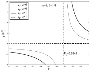
(a) $m=1$, $\beta=1/4$, $q=0,\ 1$

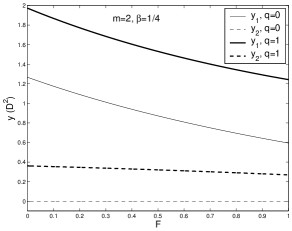
(b) $m=2$, $\beta=1/4$, $q=0,\ 1$

Figure 1: Two solution branches for $y\equiv D^{2}$ of algebraic equation (48) for $m=1,\ 2$, $\beta=1/4$ and $q=0,\ 1$. The $y_{1}$ branch is plotted in solid lines and the $y_{2}$ branch in dash lines. Panel (a): For the $m=1$ case, the relative locations of the two branches switch across the diverging point at ${F}_{c}=0.6842$. Physical solutions are those above the $y=0$ axis marked by the light dash line. For $0<{F}<{F}_{c}$, only the $y_{2}$ branch (the dash lines) is physical. For physical solutions, the enhancement of magnetic field will raise both branches but with different rate. The $y_{1}$ branch (the solid lines) is apparently influenced by the presence of the coplanar magnetic field, while the $y_{2}$ branch (the dash lines) is slightly shifted. Panel (b): For the $m=2$ case, $y_{1}$ and $y_{2}$ solutions remain always to be the upper and lower branches, respectively, and both branches are physical in the range of $0<{F}<1$. Both branches are raised by the enhancement of the coplanar magnetic field strength. The $m>2$ cases are qualitatively similar to the $m=2$ case shown in panel (b) here.

3.2 Logarithmic Spiral Configurations for Global Coplanar MHD Perturbations

In our formulation, stationary surface mass density perturbations are characterized by $S(r)\exp(-\hbox{i}m\theta)$. For aligned coplanar MHD perturbations, we took $S\propto r^{-\varepsilon}$ where $\varepsilon$ is a real exponent. In Section 3.1, we have chosen $\varepsilon=\alpha=1+2\beta$ that carries the same power-law dependence as the equilibrium disc does. For a complex $\varepsilon$, a perturbation pattern would appear spiral, that is, a logarithmic spiral in the form of $S\propto r^{-\Re(\varepsilon)}\exp[-\hbox{i}\Im(\varepsilon)\ln r]$ where $\Re(\varepsilon)$ and $\Im(\varepsilon)$ are real and imaginary parts of $\varepsilon$. To ensure the gravitational potential arising from this perturbed surface mass density being finite, we should require $-m+1<\Re(\varepsilon)<m+2$ (e.g., Qian 1992). In fact, there exists a more general class of self-consistent potential-density pairs as indicated in footnote 7 of Shen & Lou (2004b). However, for the analysis of axisymmetric stability problem in Section 3.2.1, equation (55) is used such that dispersion relation (57) derived later on is real on both sides (e.g., Lemos et al. 1991; Syer & Tremaine 1996; Shu et al. 2000). To be specific here, we consistently take the logarithmic spiral surface mass density perturbations and the resulting gravitational potentials as (Kalnajs 1971; Lemos et al. 1991; Shu et al. 2000; Lou 2002; Lou & Shen 2003; Shen & Lou 2004b; Lou & Zou 2004a)

$$\begin{split}S=\sigma r^{-3/2}\exp(\hbox{i}\xi\ln r)\ \qquad\qquad\hbox{ and }\qquad\qquad\ V=-2\pi GrS{\cal N}_{m}(\xi)\ ,\end{split}$$ (55)

where $\sigma$ is a small constant, $\xi$ is a parameter related to the radial wavenumber and the Kalnajs function ${\cal N}_{m}(\xi)$ is defined by

$${\cal N}_{m}(\xi)=\frac{1}{2}\frac{\Gamma(m/2+\hbox{i}\xi/2+1/4)\Gamma(m/2-\hbox{i}\xi/2+1/4)}{\Gamma(m/2+\hbox{i}\xi/2+3/4)\Gamma(m/2-\hbox{i}\xi/2+3/4)}$$ (56)

(Kalnajs 1971). As ${\cal N}_{m}(\xi)$ is an even function of $\xi$, a consideration of $\xi\geq 0$ would suffice. In our convention of notations, $\xi>0$ and $\xi<0$ correspond to leading and trailing logarithmic spiral waves, respectively, and $\xi\equiv kr$ relates the parameter $\xi$ to the radial wavenumber $k$. We note that ${\cal N}_{m}(\xi)$ decreases monotonically with increasing $\xi>0$, and $0<{\cal N}_{m}(\xi)<1$ for $m\geq 1$; for $m=0$, ${\cal N}_{0}(\xi)$ is positive and can be greater than 1 when $\xi$ becomes sufficiently small.

The choice of unaligned perturbations is not unique, and the perturbation potential-density pairs may involve $\beta$ parameter such that the background plus coplanar MHD perturbations are altogether scale-free (e.g., Syer & Tremaine 1996). As an example of illustration, we here presume coplanar logarithmic spiral perturbations defined by the density-potential pair (55) in the following analysis. For the specific $\beta=1/4$ case, the background surface mass density and the perturbed surface mass density bear the same radial scaling $\propto r^{-3/2}$.

3.2.1 Marginal Axisymmetric Stability Curves

We start from the axisymmetric coplanar MHD perturbation equation (40) with $\omega\neq 0$. For radial oscillations with a logarithmic potential-density pair, we presume a surface mass density $S\propto r^{-3/2+\hbox{i}\xi}$, a gravitational potential $V=-2\pi G{\cal N}_{0}rS$ and thus a radial speed $U\propto r^{1/2+\hbox{i}\xi+2\beta}$ according to the first of equation (40). After proper rearrangements, the set of equations (40) can be combined to form a single equation in terms of $U(r)$, namely

$$\begin{split}(\omega^{2}-\kappa^{2})U&=\bigg{[}\bigg{(}\frac{a^{2}}{r^{2}}-\frac{2\pi G{\cal N}_{0}\Sigma_{0}}{r}\bigg{)}\bigg{(}\frac{1}{4}+\xi^{2}\bigg{)}+\frac{C_{A}^{2}}{r^{2}}\bigg{(}\frac{1}{4}+\xi^{2}-\beta\bigg{)}\bigg{]}U\\ &=\frac{a^{2}}{r^{2}}\bigg{\{}\bigg{[}1-{F}{\cal C}{\cal N}_{0}\bigg{(}1+D^{2}-\frac{1-4\beta}{2+4\beta}q^{2}\bigg{)}\bigg{]}\bigg{(}\frac{1}{4}+\xi^{2}\bigg{)}+q^{2}\bigg{(}\frac{1}{4}+\xi^{2}-\beta\bigg{)}\bigg{\}}U\ ,\end{split}$$ (57)

where ${\cal C}=(1+2\beta)/(2\beta{\cal P}_{0})$, $a^{2}/r^{2}=\kappa^{2}/[(1+2\beta)(2-2\beta)D^{2}]$ and $\omega^{2}$ is extremely small.

By inspection, equation (57) bears similar features of the dispersion relation in the classic WKBJ regime involving magnetic field. As the right-hand side of equation (57) is real, axisymmetric instabilities first set via neutral $\omega=0$ modes. It should be emphasized that the scale-free condition is met only for neutral modes. With $\omega^{2}=0$, the marginal stability curves are then given by

$$D^{2}=\frac{\{1-{F}{\cal C}{\cal N}_{0}[1-(1-4\beta)q^{2}/(2+4\beta)]\}(\xi^{2}+1/4)+q^{2}(\xi^{2}-\beta+1/4)}{{F}{\cal C}{\cal N}_{0}(\xi^{2}+1/4)+(1+2\beta)(-2+2\beta)}\ .$$ (58)

As a check of necessary consistency, the axisymmetric marginal stability curve for an MSID when $\beta=0$ (${\cal C}=1$) then gives

$$D^{2}=\frac{[1+q^{2}-{F}{\cal N}_{0}(1-q^{2}/2)](\xi^{2}+1/4)}{{F}{\cal N}_{0}(\xi^{2}+1/4)-2}\ .$$ (59)

One can readily show that stationary dispersion relations (58) and (59) automatically satisfy inequality (17) for physical solutions $D^{2}>0$. In the MSID case with different values of $q$ parameter for magnetic field strengths, one readily obtains the marginal stability curves that separate two distinct unstable regimes, namely, the collapse regime for large radial spatial scales and the ring fragmentation regime for relatively short radial wavelengths (Lemos et al. 1991; Shen & Lou 2003, 2004a). There exists a critical $\xi=\xi_{c}$ where $D^{2}$ diverges and this $\xi_{c}$ is determined by $F{\cal N}_{0}(\xi_{c}^{2}+1/4)=2$. For $\xi<\xi_{c}$, we have $F{\cal N}_{0}(\xi^{2}+1/4)-2<0$ and thus an enhancement of $q$ tends to suppress the collapse boundary. For $\xi>\xi_{c}$, we have $F{\cal N}_{0}(\xi^{2}+1/4)-2>0$ and thus an enhancement of $q$ tends to raise the ring fragmentation boundary. In short, an enhancement of ring magnetic field tends to reduce dangers of both collapse and ring fragmentation instabilities in the MSID case.

While the enhancement of ring magnetic field tends to suppress ring fragmentation instabilities in general, it only suppresses collapse instabilities for $-1/4<\beta<1/4$ and tends to aggravate collapse instabilities for $1/4<\beta<1/2$ (see Fig. 2 for details). It has been shown that the magnetic force is radially inward and outward for $-1/4<\beta<1/4$ and $1/4<\beta<1/2$, respectively. Why does the trend of variations for the collapse-stability appear seemingly paradoxical? This situation can be understood because the unperturbed background is in an MHD radial force balance and the surface mass density, the rotation speed and the magnetic field are coupled explicitly through condition (16). Furthermore, for fast MHD density waves with $m=0$ (Lou & Fan 1998a), the gas pressure and magnetic pressure together is associated with the radial wavenumber squared, while the surface mass density and self-gravity are associated linearly with the radial wavenumber (see the first line of dispersion relation 57 with small $\omega^{2}$). For $-1/4<\beta<1/4$, the surface mass density becomes smaller for stronger magnetic field strength, while for $1/4<\beta<1/2$, the situation reverses. For the ring fragmentation instability at relatively large radial wavenumbers, the dominant magnetic pressure effect tends to stabilize the disc. For the Jeans collapse instability at relatively small radial wavenumbers, the dominant self-gravity effect is proportional to the background surface mass density; the roles of magnetic field for two different situations can then be readily understood. It is the coupling effect between the surface mass density and the magnetic field of the background that gives rise to this collapse feature.

The marginal stability curves for scale-free discs with $\beta\in(-1/4,1/2)$ and without magnetic fields are

$$D^{2}=\frac{(1-{F}{\cal C}{\cal N}_{0})(\xi^{2}+1/4)}{{F}{\cal C}{\cal N}_{0}(\xi^{2}+1/4)+2(2\beta+1)(\beta-1)}\ ,$$ (60)

that are consistent with those for the single-disc case of Shen & Lou (2004b; e.g., see their subsection 3.2.1).

The marginal axisymmetric stability curves generally consist two branches, namely, the collapse branch and the ring-fragmentation branch (Lemos et al. 1991; Shu et al. 2000; Lou 2002; Lou & Shen 2003; Shen & Lou 2003). The lowest value of $D^{2}$ for stability is the maximum of the collapse branch and the highest value of $D^{2}$ for stability is the minimum of the ring-fragmentation branch. We note that the maximum of the collapse branch is always located at $\xi=0$ for $\beta\geq-0.104$, while for $\beta<-0.104$ the maximum of the collapse branch may locate at $\xi>0$ with $\xi=0$ corresponding to a local minimum of $D^{2}$. It was proven in Appendix C of Shen & Lou (2004b) that $\xi=0$ is always a local extremum for $D^{2}$. Variations of the stable range for $D^{2}$ with parameters $F$, $\beta$ and $q$ are shown in panels (a) and (b) of Fig. 2. Finally we note that the axisymmetric destabilization involves only the fast MHD wave branch because the slow MHD wave branch is negative and thus unphysical. For non-axisymmetric ($m\neq 0$) perturbations, both fast and slow MHD density waves are possible and stationary global configurations may represent transitions from stable to unstable situations (e.g., Shu et al. 2000). Here, the stability of our slow MHD density waves differs from those models involving finite disc thickness where either vertical or horizontal weak magnetic fields may induce Velikhov-Chandrasekhar-Balbus-Hawley instability and magneto-rotational instabilities (MRI) through slow MHD modes (Chandrasekhar 1961; Balbus & Hawley 1998; Kim & Ostriker 2000; Lou, Yuan & Fan 2001).

It would be interesting to recall the axisymmetric stability analysis in the WKBJ approximation. The local dispersion relation for fast MHD waves in an azimuthal magnetic field is (Fan & Lou 1996)

$$(\omega-m\Omega)^{2}=\kappa^{2}+k^{2}(C_{A}^{2}+a^{2}-2\pi G\Sigma_{0}/|k|)\ ,$$ (61)

where $k$ is the radial wavenumber and other notations have the conventional meanings. Equation (61) gives the marginal stability curve for axisymmetric $m=0$ perturbations as

$$\kappa^{2}+k^{2}(C_{A}^{2}+a^{2}-2\pi G\Sigma_{0}/|k|)=0\ .$$ (62)

By using scale-free disc equilibrium condition (16) and inserting $\xi\cong|k|r$ for large $k$ and $\xi$ into dispersion relation (62), we readily obtain the corresponding marginal stability curve in the WKBJ regime as

$$D^{2}=\frac{(1+q^{2})\xi^{2}-F{\cal C}[1-(1-4\beta)q^{2}/(2+4\beta)]\xi}{F{\cal C}\xi+(1+2\beta)(-2+2\beta)}\ ,$$ (63)

which bears a strong resemblance to expression (58) of our global analysis, especially in view of the asymptotic expression for ${\cal N}_{m}(\xi)$, namely

$${\cal N}_{m}(\xi)\approx(m^{2}+\xi^{2}+1/4)^{-1/2}$$ (64)

when $m^{2}+\xi^{2}\gg 1$. Another equivalent way of this comparison is to note the parallel terms in the WKBJ condition (62) and in the first line of the corresponding global condition (57), also in reference to the above asymptotic expression for ${\cal N}_{m}(\xi)$. A specific illustrating example of such a comparison is shown in Fig. 3 with parameters $\beta=0$ (${\cal C}=1$; flat rotation curve), $F=1$ (full disc) and $q=0.1$. In the short-wavelength limit (i.e., $\xi\gg 1$), the WKBJ approximation is well justified and the results are qualitatively consistent, while in the long-wavelength of Jeans collapse regime, the WKBJ analysis differs from the global exact treatment significantly.

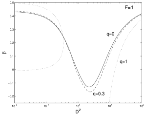
(a) Stability boundary curves of $\beta$ versus $D^{2}$ for full discs of $F=1$ with different values of $q$ parameter.

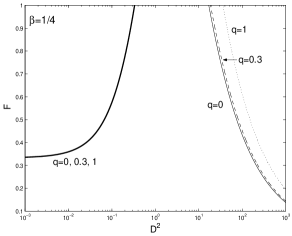
(b) Stability boundary curves of $F$ versus $D^{2}$ for $\beta=1/4$ discs with different values of $q$ parameter.

Figure 2: Variations of the stable $D^{2}$ range for (a) full discs with $F=1$ and (b) $\beta=1/4$ discs. The solid, dashed and dotted curves stand for $q=0$, $0.3$ and $1$, respectively. For specific ranges of either $\beta\in(-1/4,1/2)$ [see panel (a)] or $F\in(0,1]$ [see panel (b)], a horizontal line intercepts the stability boundary curves at two values of $D^{2}$ and the stable range of $D^{2}$ lies between the two intersection points. The $D^{2}$ range to the left of the smaller intersection point corresponds to the collapse regime and the $D^{2}$ range to the right of the larger intersection point corresponds to the ring-fragmentation regime. Panel (a): For full discs with $F=1$, an enhancement of magnetic field tends to suppress ring-fragmentation instabilities in general. Meanwhile, an enhancement of magnetic field tends to suppress collapse instabilities for $-1/4<\beta<1/4$ but to aggravate collapse instabilities for $1/4<\beta<1/2$ and bears no effects on collapse instabilities when $\beta=1/4$. For stability curves of moderate magnetic field strengths (e.g., the solid and dashed curves), the disc system becomes less stable for both instabilities when $\beta$ decreases. As $\beta$ becomes sufficiently small, there will be no stable range for $D^{2}$ [e.g., for $q=0$ without magnetic field, this lower limit of $\beta$ is $\sim-0.130$ as derived in Appendix D of Shen & Lou (2004b)]. For a stronger magnetic field (e.g., the dotted curve), the trend for ring-fragmentation instabilities remains the same while the trend for collapse instabilities is different depending on whether $\beta<1/4$ or not; the collapse regime may disappear completely when $\beta$ becomes small enough. Panel (b): For $\beta=1/4$ discs, an enhancement of magnetic field tends to suppress the ring-fragmentation regime but does not influence the collapse regime because the maximum of the collapse branch remains always at $\xi=0$ such that the heavy solid curve on the left actually represents a superposition of the three $q$ curves. A decrease of $F$ (i.e., a more massive dark-matter halo) tends to suppress both instabilities.

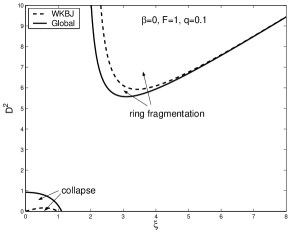
Figure 3: A comparison of the global axisymmetric stability treatment (solid curves) with the local WKBJ approach (dashed curves) for the case of $\beta=0$, $F=1$ and $q=0.1$. The marginal stability curves for the long-wavelength Jeans collapse and the short-wavelength ring fragmentation regimes are denoted. For $\xi\gg 1$ (i.e., the short-wavelength limit), the WKBJ approximation is well applicable, while for small $\xi$ the results in the WKBJ approximation deviates from those of the exact global treatment considerably (see Shen & Lou 2003, 2004b).

3.2.2 Unaligned Logarithmic Spiral Cases with $m\geq 1$

In parallel with the aligned $m\geq 1$ cases, we now construct unaligned logarithmic spiral solutions from coplanar MHD perturbation equations (36)$-$(39). For the density-potential pair $S\propto r^{-3/2+\hbox{i}\xi}$ and $V=-2\pi G{\cal N}_{m}rS$, we then have radial flow speed $U\propto r^{-1/2+\beta+\hbox{i}\xi}$ and $z-$component specific angular momentum $J\propto r^{1/2+\beta+\hbox{i}\xi}$. Coplanar MHD perturbation equations $(\ref{stationary1})-(\ref{stationary4})$ can therefore be written in the forms of

$$\begin{split}&m\Omega S+\frac{-1/2-\beta+\hbox{i}\xi}{r}\Sigma_{0}\hbox{i}U+\frac{m\Sigma_{0}}{r^{2}}J=0\ ,\\ &m\Omega\hbox{i}U+\frac{2\Omega}{r}J=\bigg{(}\frac{a^{2}}{r\Sigma_{0}}-2\pi G{\cal N}_{m}\bigg{)}\bigg{(}-\frac{1}{2}+\hbox{i}\xi\bigg{)}S-\frac{(1-4\beta)C_{A}^{2}}{2\Sigma_{0}r}S-\frac{C_{A}^{2}}{m\Omega r^{2}}\bigg{[}\bigg{(}\frac{1}{2}-2\beta\bigg{)}\hbox{i}\xi-\xi^{2}-m^{2}\bigg{]}\hbox{i}U\ ,\\ &m\Omega J+r(1-\beta)\Omega\hbox{i}U=m\bigg{(}2\pi G{\cal N}_{m}-\frac{a^{2}}{r\Sigma_{0}}\bigg{)}rS+\frac{C_{A}^{2}(1-4\beta)}{2\Omega r}\hbox{i}U\ ,\\ &Z=-\hbox{i}\xi\frac{B_{0}iU}{m\Omega r}\ ,\qquad\qquad\qquad\qquad R=\frac{B_{0}U}{\Omega r}\ .\end{split}$$ (65)

The first three equations of set (65) immediately lead to

$$\begin{split}a_{1}S+b_{1}\hbox{i}U+c_{1}J=0\ ,\qquad\qquad a_{2}S+b_{2}\hbox{i}U+c_{2}J=0\ ,\qquad\qquad a_{3}S+b_{3}\hbox{i}U+c_{3}J=0\ ,\end{split}$$ (66)

where coefficients $a_{i}$, $b_{i}$ and $c_{i}$ ($i=1,2,3$) are explicitly defined by

$$\begin{split}&a_{1}\equiv m\Omega\ ,\qquad\qquad\qquad b_{1}\equiv\frac{-1/2-\beta+\hbox{i}\xi}{r}\Sigma_{0}\ ,\qquad\qquad\qquad c_{1}\equiv\frac{m\Sigma_{0}}{r^{2}}\ ,\\ &a_{2}\equiv\frac{(1-4\beta)C_{A}^{2}}{2\Sigma_{0}r}+\bigg{(}-\frac{1}{2}+\hbox{i}\xi\bigg{)}\bigg{(}2\pi G{\cal N}_{m}-\frac{a^{2}}{\Sigma_{0}r}\bigg{)}\ ,\qquad b_{2}\equiv m\Omega+\frac{[(-2\beta+1/2)\hbox{i}\xi-\xi^{2}-m^{2}]C_{A}^{2}}{m\Omega r^{2}}\ ,\qquad c_{2}\equiv\frac{2\Omega}{r}\ ,\\ &a_{3}\equiv-mr\bigg{(}2\pi G{\cal N}_{m}-\frac{a^{2}}{\Sigma_{0}r}\bigg{)}\ ,\qquad\qquad b_{3}\equiv r(1-\beta)\Omega-\frac{(1-4\beta)C_{A}^{2}}{2\Omega r}\ ,\qquad\qquad c_{3}\equiv m\Omega\ .\end{split}$$ (67)

For nontrivial solutions of the set of homogeneous algebraic equations (66), the determinant must vanish

$$a_{1}-\frac{b_{1}(a_{2}c_{3}-a_{3}c_{2})}{b_{2}c_{3}-b_{3}c_{2}}+\frac{c_{1}(a_{2}b_{3}-a_{3}b_{2})}{b_{2}c_{3}-b_{3}c_{2}}=0\ .$$ (68)

By using the set of expressions (67) and applying equilibrium conditions (16), we obtain the final dispersion relation for stationary logarithmic spiral $m\geq 1$ MHD configurations in the form of a quadratic equation in terms of $y\equiv D^{2}$, namely

$$C_{2}y^{2}+C_{1}y+C_{0}=0\ ,$$ (69)

where the coefficients $C_{2}$, $C_{1}$ and $C_{0}$ are explicitly defined by

$$\begin{split}&C_{2}\equiv{\cal H}_{m}\ ,\\ &C_{1}\equiv-\bigg{[}\frac{(3-4\beta)m^{2}-8\beta^{2}-(4\xi^{2}-3)\beta+3\xi^{2}-1/4}{2(1+2\beta)}{F}{\cal C}{\cal N}_{m}+m^{2}+\xi^{2}-\frac{7}{4}+7\beta\bigg{]}q^{2}-{\cal A}_{m}(1-{F}{\cal C}{\cal N}_{m})\ ,\\ &C_{0}\equiv-\frac{(1-4\beta)}{4(1+2\beta)}\bigg{[}\frac{(-2m^{2}-2\xi^{2}-2\beta+1/2)}{(1+2\beta)}{F}{\cal C}{\cal N}_{m}+1-4\beta\bigg{]}q^{4}-\frac{(-2m^{2}-2\xi^{2}-2\beta+1/2)}{2(1+2\beta)}(1-{F}{\cal C}{\cal N}_{m})q^{2}\ ,\end{split}$$ (70)

with auxiliary parameters defined by

$$\begin{split}&{\cal A}_{m}\equiv m^{2}+\xi^{2}+\frac{1}{4}+2\beta\ ,\qquad{\cal B}_{m}\equiv(1+2\beta)(m^{2}-2+2\beta)\ ,\qquad{\cal C}\equiv\frac{(1+2\beta)}{2\beta{\cal P}_{0}}\ ,\qquad{\cal H}_{m}\equiv F{\cal C}{\cal N}_{m}{\cal A}_{m}+{\cal B}_{m}\ \\ \end{split}$$ (71)

that are the same as those in Shen & Lou (2004b) for unaligned logarithmic spiral cases. For a positive determinant $\Delta\equiv C_{1}^{2}-4C_{2}C_{0}>0$, the two real solutions to quadratic equation (69) are given by

$$y_{1}=\frac{-C_{1}+\Delta^{1/2}}{2C_{2}}\ \ \qquad\qquad\hbox{ and }\qquad\qquad\ y_{2}=\frac{-C_{1}-\Delta^{1/2}}{2C_{2}}\ .$$ (72)

Similar to $m\geq 1$ cases for aligned perturbations in the limit of vanishing magnetic field (i.e., $q\rightarrow 0$), equation (69) reduces to

$${\cal H}_{m}y^{2}-{\cal A}_{m}(1-{F}{\cal C}{\cal N}_{m})y=0\$$ (73)

that leads to a nontrivial solution

$$D^{2}=y_{1}=\frac{(1-{F}{\cal C}{\cal N}_{m}){\cal A}_{m}}{{\cal H}_{m}}\ .$$ (74)

Solution (74) is exactly the same result for the single-disc case discussed in Section 3.2 of Shen & Lou (2004b). Another limiting regime of $\beta\rightarrow 0$ has been analyzed by Lou (2002) for global stationary perturbation structures in a single MSID.

3.2.3 Force-Free Magnetized Discs with $\beta=1/4$

For stationary spiral MHD configurations, we here analyze again the $\beta=1/4$ case as a specific example of illustration. The background equilibrium ring magnetic field is force-free and inequality (17) is satisfied. The determinant $\Delta$ of quadratic equation (69) remains always positive as shown in Appendix A and hence two real solutions of $y=D^{2}$ to equation (69) exist. In parallel with the aligned $\beta=1/4$ case, we solve quadratic equation (69) for given values of parameter ${F}$ and display in diagrams the two branches of solutions $y_{1}$ and $y_{2}$ ($y\equiv D^{2}$) versus $\xi$ variation.

As ${\cal B}_{1}<0$ for $m=1$ and when ${F}$ becomes sufficiently small, there is a diverging point for $y_{1}\equiv D^{2}$ solution where $C_{2}={\cal H}_{1}=0$. Since ${\cal H}_{1}$ increases monotonically with increasing $\xi$ for $\xi\geq 0$ and attains its minimum value at $\xi=0$ (${\cal H}_{1}$ is an even function of $\xi$; see Appendix C of Shen & Lou 2004b), the existence of such a critical point $\xi_{c}$ for a diverging $y\equiv D^{2}$ requires

$${F}{\cal C}{\cal N}_{1}(0)(5/4+2\beta)+4\beta^{2}-1<0\ .$$ (75)

For the specific $\beta=1/4$ case, this inequality (75) implies a critical ${F}$ value of ${F}_{c}=3/[7{\cal C}{\cal N}_{1}(0)]$ below which there exists one divergent point of $\xi_{c}$ where $y_{1}$ diverges. Numerically, we have determined ${F}_{c}\simeq 0.6842$ [note that this ${F}_{c}$ is of the same value as that of the aligned $m=1$ case because ${\cal N}_{1}(0)={\cal P}_{1}(1/4)$]. For selected $F$ values in the range of $0<{F}<{F}_{c}$, the corresponding critical $\xi_{c}$ at which ${\cal H}_{1}=0$ can be numerically computed; for example, we have $\xi_{c}=1.428$ for $F=0.5$.

It becomes much simpler for cases of $m\geq 2$ because $C_{2}$ remains always positive and there is no diverging point for $D^{2}$ solutions. Therefore, $y_{1}$ and $y_{2}$ remain always as the upper and lower branches, respectively. For $m=1$ and $m=2$ cases with different parameters of ${F}$ and $q$, we show in four panels $(a)-(d)$ of Fig. 4 relevant curves of $y\equiv D^{2}$ versus $\xi$ variation to illustrate the basic features. To be more explicit for the case of $\beta=1/4$ in quadratic equation (69), we write

$$\!\!\!\begin{split}&\qquad\qquad\bigg{[}{F}{\cal C}{\cal N}_{m}\bigg{(}m^{2}+\xi^{2}+\frac{3}{4}\bigg{)}+\frac{3}{2}\bigg{(}m^{2}-\frac{3}{2}\bigg{)}\bigg{]}D^{4}-\bigg{[}(m^{2}+\xi^{2})\bigg{(}\frac{2}{3}{F}{\cal C}{\cal N}_{m}+1\bigg{)}q^{2}\\ &\hbox{ }\qquad\qquad\qquad\qquad\qquad\qquad\qquad+\bigg{(}m^{2}+\xi^{2}+\frac{3}{4}\bigg{)}(1-{F}{\cal C}{\cal N}_{m})\bigg{]}D^{2}+\frac{2}{3}(m^{2}+\xi^{2})(1-{F}{\cal C}{\cal N}_{m})q^{2}=0\ ,\end{split}$$ (76)

where auxiliary parameters ${\cal N}_{m}$, ${\cal A}_{m}$, ${\cal B}_{m}$, ${\cal C}$ and ${\cal H}_{m}$ are all evaluated for the special value of $\beta=1/4$.

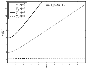
(a) $m=1$, $\beta=1/4$, ${F}=1$, $q=0,\ 1$

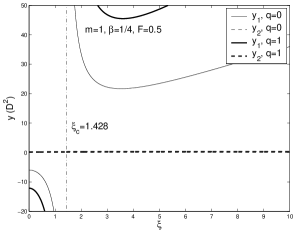
(b) $m=1$, $\beta=1/4$, ${F}=0.5$, $q=0,\ 1$

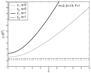
(c) $m=2$, $\beta=1/4$, ${F}=1$, $q=0,\ 1$

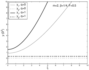
(d) $m=2$, $\beta=1/4$, ${F}=0.5$, $q=0,\ 1$

Figure 4: Two $D^{2}$ solution branches $y_{1}$ and $y_{2}$ of quadratic equation (69) for $m=1,\ 2$, $\beta=1/4$, $F=1,\ 0.5$ and $q=0,\ 1$. The $y_{1}$ and $y_{2}$ branches are plotted in solid and dashed lines, respectively. Parameters adopted are shown in panels $(a)-(c)$.

4 Perturbation Phase Relationships and Angular Momentum Transfer

For multi-wavelength observations of nearby spiral galaxies (Sofue et al. 1986; Kronberg 1994; Beck et al. 1996), it is possible to identify large-scale spatial phase relationships of spiral patterns using various observational diagnostics (e.g., Mathewson et al. 1972; Visser 1980a, b; Neininger 1992; Beck & Hoernes 1996; Frick et al. 2000, 2001; Ferrière 2001; Lou et al. 2002). For this reason, we derive below spatial phase relationships for various coplanar MHD perturbation variables, keeping in mind of potential applications to magnetized spiral galaxies (e.g., Fan & Lou 1996; Lou & Fan 1998a).

4.1 General Perturbation Phase Relationships for both Aligned and Spiral Cases

Here we systematically examine the spatial phase relationships among enhancements of gas surface mass density, magnetic field and velocity perturbations by analysing the relationships among $S$, $Z$, $R$, $J$ and $iU$ for aligned and logarithmic spiral cases, separately. Starting from the set of homogeneous algebraic equations (44) for the aligned cases, we obtain the relationships among $S$, $U$ and $J$ in the following, namely

$$\frac{\hbox{i}U}{S}=\frac{c_{3}a_{1}-c_{1}a_{3}}{c_{1}b_{3}-c_{3}b_{1}}\ ,\ \qquad\qquad\qquad\frac{J}{S}=\frac{a_{2}b_{1}-a_{1}b_{2}}{c_{1}b_{2}-c_{2}b_{1}}\ ,\$$ (77)

where $a_{i}$, $b_{i}$ and $c_{i}$ ($i=1,2,3$) are defined by expressions (45). By using definitions (45) and equations (43), we obtain

$$\begin{split}&\frac{\hbox{i}U}{S}=\frac{m\Omega r}{\Sigma_{0}}\Theta_{A}\ ,\quad\qquad\frac{Z}{S}=-\frac{(1/2-2\beta)B_{0}}{\Sigma_{0}}\Theta_{A}\ ,\quad\qquad\frac{\hbox{i}R}{S}=\frac{mB_{0}}{\Sigma_{0}}\Theta_{A}\ ,\quad\qquad\frac{J}{S}=-\frac{\Omega r^{2}}{\Sigma_{0}}(1-3\beta\Theta_{A})\ \end{split}$$ (78)

for the aligned cases, where the common dimensionless real factor $\Theta_{A}$ is defined below by

$$\Theta_{A}\equiv\frac{a^{2}-2\pi G{\cal P}_{m}\Sigma_{0}r-\Omega^{2}r^{2}}{(1/2-2\beta)C_{A}^{2}-(1+2\beta)\Omega^{2}r^{2}}\ .$$ (79)

Similarly, by using the set of homogeneous algebraic equations (66), definitions (67) and equations (65), we readily derive for the cases of global stationary logarithmic spiral configurations

$$\begin{split}&\frac{\hbox{i}U}{S}=\frac{m\Omega r}{\Sigma_{0}}\Theta_{S}\ ,\qquad\quad\frac{Z}{S}=-\frac{\hbox{i}\xi B_{0}}{\Sigma_{0}}\Theta_{S}\ ,\qquad\quad\frac{\hbox{i}R}{S}=\frac{mB_{0}}{\Sigma_{0}}\Theta_{S}\ ,\qquad\quad\frac{J}{S}=-\frac{\Omega r^{2}}{\Sigma_{0}}\bigg{[}1+\bigg{(}-\frac{1}{2}-\beta+\hbox{i}\xi\bigg{)}\Theta_{S}\bigg{]}\ ,\end{split}$$ (80)

where the common dimensionless complex factor $\Theta_{S}$ is defined below by

$$\Theta_{S}\equiv\frac{a^{2}-2\pi G{\cal N}_{m}\Sigma_{0}r-\Omega^{2}r^{2}}{(1/2-2\beta)C_{A}^{2}-(3-2\hbox{i}\xi)\Omega^{2}r^{2}}\ .$$ (81)

The two sets of algebraic equations (78) and (80) are the most general phase relationships for aligned and logarithmic spiral cases, respectively. Once a $\beta$ value is specified and a particular $D^{2}$ for a stationary solution inserted, we immediately obtain the phase relationship between any two perturbation variables. As an example of illustration, we examine again the special $\beta=1/4$ case and determine the relevant phase relationships in the next subsection.

4.2 The $\beta=1/4$ Force-Free Case

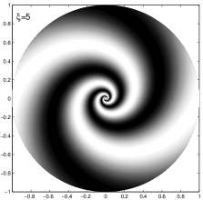
(a) Fractional perturbed mass density in a gray-scale plot as a spatial phase reference for either fast or slow MHD density wave modes

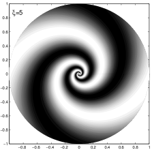
(b) Fractional perturbed azimuthal magnetic field in a gray-scale plot for the fast MHD density wave mode

(c) Fractional perturbed azimuthal magnetic field in a gray-scale plot for the slow MHD density wave mode

Figure 6: Phase relationship between the perturbed surface mass density and the azimuthal magnetic field for the logarithmic spiral $m=2$ case (an effective radial wavenumber $\xi=5$) for the specific case of $\beta=1/4$. Shown in above three panels in order are the fractional perturbed surface mass density and azimuthal magnetic field gray-scale plots (i.e., divided by the radial scaling of their respective equilibrium quantities with $r^{-3/2}$ for the surface mass density and $r^{-1}$ for the azimuthal magnetic field). The brightest regions correspond to the most density enhancement. Panel (a) is for the perturbed relative surface mass density; panels (b) and (c) are for the perturbed azimuthal magnetic fields for the fast and slow MHD perturbations, respectively. According to equations (84) and (80), there is a phase shift of $\sim-0.093\pi$ ($\sim 0.907\pi$) for the fast (slow) MHD perturbation mode. Since $m=2$, the pattern appears a rotation of half of the phase shift. For the fast MHD density wave mode, the magnetic field enhancement roughly follows the spirals of surface mass enhancement. For the slow MHD density wave mode, the density spiral arms and the magnetic spiral arms largely interlace with each other. For $\xi\gg 1$, the phase pattern relationships become those in the usual WKBJ regime (e.g., Fan & Lou 1996; Lou & Fan 1998a).

When $\beta=1/4$, the results of phase relations derived in the last subsection 4.1 can be simplified considerably as all terms involving the factor $1/2-2\beta$ vanish. Meanwhile, inequality (17) is automatically satisfied. The only requirement for a physical $D^{2}$ solution is simply $D^{2}>0$. As already noted in subsections 3.1.3 and 3.2.3, there are two branches of $D^{2}$ solutions. We insert relevant physical $D^{2}$ solutions in equations (78) and (80) to determine phase relationships among perturbation variables. In particular, we are interested in the phase relationship between the perturbed surface mass density and the perturbed azimuthal magnetic field. We now analyze below this mass-magnetic field phase relationships for aligned and spiral cases, separately. Some illustrative examples are shown in Fig. 5 and Fig. 6 to provide more direct visual impressions.

4.2.1 Aligned Cases

For aligned $\beta=1/4$ cases, we readily find $Z=0$ which means the azimuthal magnetic field remains unchanged. From equation (78), we derive

$$\hbox{i}R/S\propto 3D^{2}/2-1+{F}{\cal C}{\cal P}_{m}(1+D^{2})=({F}{\cal C}{\cal P}_{m}+3/2)D^{2}-(1-{F}{\cal C}{\cal P}_{m})\ .$$ (82)

Meanwhile, equation (54) can be rewritten in the form of

$$\frac{m^{2}q^{2}(1+2{F}{\cal C}{\cal P}_{m}/3)}{(m^{2}+3/4)[F{\cal C}{\cal P}_{m}+3(m^{2}-3/2)/(2m^{2}+3/2)]}=\frac{D^{2}\{D^{2}-(1-F{\cal C}{\cal P}_{m})/[F{\cal C}{\cal P}_{m}+3(m^{2}-3/2)/(2m^{2}+3/2)]\}}{D^{2}-(1-F{\cal C}{\cal P}_{m})/(F{\cal C}{\cal P}_{m}+3/2)}\ ,$$ (83)

that contains two distinct $D^{2}$ solutions according to subsection 3.1.3, namely, the plus-sign solution $y_{1}$ and the minus-sign solution $y_{2}$ in the solution form (51), respectively. As shown in Appendix B, we emphasize that the plus-sign solution $y_{1}$ (if positive and thus physical) makes $D^{2}-(1-F{\cal C}{\cal P}_{m})/(F{\cal C}{\cal P}_{m}+3/2)>0$ and the minus-sign solution $y_{2}$ makes $D^{2}-(1-F{\cal C}{\cal P}_{m})/(F{\cal C}{\cal P}_{m}+3/2)<0$ on the right-hand side of equation (83), respectively. Therefore, the two branches of $D^{2}$ solutions (if positive and thus physical) will give either $\hbox{i}R/S>0$ for the plus-sign $y_{1}$ solution or $\hbox{i}R/S<0$ for the minus-sign $y_{2}$ solution.

4.2.2 Cases of Stationary Logarithmic Spiral Configurations

For spiral cases with $\beta=1/4$, we readily obtain from equations (80) and (81) that

$$\Theta_{S}\propto[({F}{\cal C}{\cal N}_{m}+3/2)D^{2}-(1-{\cal F}{\cal C}{\cal N}_{m})](3+2\hbox{i}\xi)\ .$$ (84)

Following the same procedure, we can show that the two branches of $D^{2}$ solutions, namely, the plus-sign solution $y_{1}$ and the minus-sign solution $y_{2}$ given by equation (72), if positive and thus physical, correspond to the factor $(F{\cal C}{\cal N}_{m}+3/2)D^{2}-(1-F{\cal C}{\cal N}_{m})$ being positive and negative, respectively (see Appendix B for a detailed proof). We now examine the phase relationship between coplanar perturbation enhancements of surface mass density and magnetic field.

In the short-wavelength limit (i.e., $\xi\gg 1$ with a logarithmic spiral pattern tightly wound), we have $Z/S\propto\pm 1$ and $R/S\propto\pm 1$ where the plus- and minus-signs correspond to the $y_{1}$ and $y_{2}$ solutions, respectively. Therefore, the phase relations between perturbation enhancements of surface mass density and magnetic field are in-phase for the $y_{1}$ solution (if positive and physical) and out-of-phase for the $y_{2}$ solution. For $m\geq 2$, $y_{1}$ remains always greater than $y_{2}$. In contexts of magnetized spiral galaxies, these solution properties in the WKBJ regime are consistent with the physical identifications of the $y_{1}$ mode with a stationary fast MHD density wave and the $y_{2}$ mode with a stationary slow MHD density wave, respectively (Fan & Lou 1996; Lou & Fan 1998a; Lou & Fan 2002). It is now possible to model magnetized spiral galaxies in terms of coplanar stationary fast and slow MHD density waves with more general rotation curves including the case of a flat rotation curve for a magnetized singular isothermal disc (Shu et al. 2000; Lou 2002; Lou & Fan 2002; Lou & Zou 2004a, b; Lou & Wu 2004).

In the long-wavelength limit (i.e., $\xi\ll 1$ with a logarithmic spiral pattern widely open), we have $Z/S\propto\mp\hbox{i}$ and $R/S\propto\mp\hbox{i}$ where the minus- and plus-signs correspond to the $y_{1}$ and $y_{2}$ solutions, respectively. Therefore, the coplanar perturbation enhancement of magnetic field is either ahead of or lagging behind the perturbation enhancement of surface mass density by a phase difference of $\sim\pi/2$.

For intermediate radial wavelengths, the phase difference between perturbation enhancements of surface mass density and magnetic field in a logarithmic spiral pattern can be readily determined for given specific conditions.

On the basis of our model analysis here, it appears that except for global stationary fast MHD density waves in the extreme WKBJ regime, magnetic and gas spiral arms tend to be phase shifted relative to each other for a global stationary logarithmic spiral pattern for a much broader set of rotation curves including the special case of a flat rotation curve.

(a) Fractional perturbed surface mass density gray-scale plot as a spatial phase reference for either fast or slow MHD density wave modes

(b) Fractional perturbed radial magnetic field in a gray-scale plot for the fast MHD density wave mode

(c) Fractional perturbed radial magnetic field in a gray-scale plot for the slow MHD slow density wave mode

Figure 5: Spatial phase relationship between the perturbed surface mass density and the radial magnetic field for the aligned $m=2$ bar-like case for the specific case of $\beta=1/4$. Shown in the figures above are the fractional perturbed surface mass density and magnetic field contours (i.e., perturbation variables divided by the radial scalings of their equilibrium quantities with $r^{-3/2}$ for the surface mass density and $r^{-1}$ for the azimuthal magnetic field). The brightest regions correspond to the strongest density enhancement. Panel (a) is for the perturbed relative surface mass density; panels (b) and (c) are for the perturbed relative radial magnetic fields for the fast and slow MHD perturbations respectively. According to equation (82), there is a phase shift of $\mp\pi/2$ for the global stationary fast and slow MHD density wave modes. Since $m=2$, the pattern appears a rotation of $\mp\pi/4$.

4.3 Angular Momentum Conservation

One can readily show that for aligned global stationary MHD perturbation configurations, there is no net radial angular momentum flux as aligned stationary MHD density waves do not propagate radially (Shu et al. 2000; Lou 2002). We here briefly discuss the process of angular momentum transfer in association with the stationary logarithmic spiral MHD modes obtained in this paper. According to the analyses of Lynden-Bell & Kalnajs (1972) and Fan & Lou (1999), the total angular momentum flux carried by coplanar MHD density waves should contain three separate contributions, namely, the advective transport flux $\Lambda^{A}$ defined by

$$\Lambda^{A}\equiv r^{2}\Sigma_{0}\int_{0}^{2\pi}d\theta\Re(u_{1})\Re(j_{1}/r)\ ,$$ (85)

the gravity torque flux $\Lambda^{G}$ defined by

$$\Lambda^{G}\equiv\frac{1}{4\pi G}\int_{0}^{2\pi}d\theta\int_{-\infty}^{\infty}dzr\bigg{[}\frac{\partial\Re(\phi_{1})}{\partial\theta}\bigg{]}\bigg{[}\frac{\partial\Re(\phi_{1})}{\partial r}\bigg{]}\$$ (86)

and the magnetic torque flux $\Lambda^{B}$ defined by

$$\Lambda^{B}\equiv-\frac{r^{2}}{4\pi}\int_{0}^{2\pi}d\theta\int_{-\infty}^{\infty}dz\Re(b_{r})\Re(b_{\theta})\ .$$ (87)

The perturbed three-dimensional gravitational potential $\phi_{1}(r,\theta,z)$ associated with a Fourier component of a coplanar logarithmic spiral perturbation in surface mass density $\Sigma_{1}=\sigma r^{-3/2+\hbox{i}\xi}e^{-im\theta}$ is then

$$\phi_{1}(r,\theta,z)=-2\pi G\sigma e^{-\hbox{i}m\theta}\int_{0}^{\infty}dke^{-k|z|}J_{m}(kr)\int_{0}^{\infty}r_{a}^{-1/2+\hbox{i}\xi}J_{m}(kr_{a})dr_{a}\ ,$$ (88)

where $J_{m}(u)$ is the cylindrical Bessel function of order $m$ with an argument $u$ (e.g., Binney & Tremaine 1987). In fact, integral (88) gives a simple form of Kalnajs function in the disc plane at $z=0$ with the real part of $\phi_{1}(r,\theta,z)$ explicitly given by

$$\Re(\phi_{1})=-2\pi G\sigma\int_{0}^{\infty}dke^{-k|z|}J_{m}(kr)\int_{0}^{\infty}r_{a}^{-1/2}\cos(m\theta-\xi\ln r_{a})J_{m}(kr_{a})dr_{a}\ .$$ (89)

It is fairly straightforward to show that $\Lambda^{A}$ and $\Lambda^{B}$ are independent of $r$ where the phase relationships for stationary logarithmic spiral cases derived in Section 4.1 have been use. While mathematically tedious, one can further show that $\Lambda^{G}$ is also independent of $r$ (see Appendix C). Therefore, the total angular momentum flux $\Lambda^{A}+\Lambda^{G}+\Lambda^{B}$ remains constant at all radii, a natural result of angular momentum conservation given that perturbation surface mass density falls off as $r^{-3/2}$. Therefore, in order to maintain a stationary logarithmic spiral pattern, there must be a source or a sink at the disc center. The perturbation energy flux, however, is zero at all radii for the stationary coplanar MHD configurations [see equation (4.17) of Fan & Lou (1999) in the WKBJ regime]. The mass flux is also zero at all radii since the first-order mass flux $\int_{0}^{2\pi}\Sigma_{0}u_{1}rd\theta=0$, and the second-order mass flux $\int_{0}^{2\pi}(\Sigma_{1}u_{1}+\Sigma_{0}u_{2})rd\theta=0$ [where $u_{2}$ is the second-order perturbed radial velocity, this equation holds due to the second-order mass conservation (Fan & Lou 1999)]. Therefore our model result differs from that of Spruit (1987) for stationary logarithmic spiral shocks, where only the gravity of the central object is considered. In Spruit’s model, there is a net mass accretion through the disc and an effective viscosity parameter “$\alpha$” (Shakura & Sunyaev 1973) may be estimated.

Physically, the central source of angular momentum required to sustain global stationary logarithmic spiral patterns may be plausibly identified with a fast spinning supermassive black hole (SMBH) in the nucleus of a spiral galaxy. The Kerr spacetime associated with such a spinning SMBH excites and sustains MHD density waves in the surrounding disc through a long-range gravitational interaction. For trailing spiral patterns, a net flux of angular momentum is transport radially outward in the disc. Conceptually, this process should cause the spinning SMBH to gradually slow down, entirely analogous to the spin-down of a rotating neutron star by emitting electromagnetic waves that carry a net angular momentum away.

5 Summary

In this paper, we have explored and analyzed stationary perturbation structures in coplanarly magnetized razor-thin scale-free discs in a more general manner. To be specific, we start from a rotational and magnetized background equilibrium of axisymmetry that is dynamically self-consistent with a surface mass density $\Sigma_{0}\propto r^{-\alpha}$, a rotation curve $v_{0}\propto r^{-\beta}$, a purely azimuthal (ring) magnetic field $B_{0}\propto r^{-\gamma}$ with a vertically integrated barotropic equation of state in the form of $\Pi=K\Sigma^{n}$. The radial force balance at all radii in an MHD disc implies several simple relationships among these power indices $\alpha$, $\beta$, $\gamma$ and $n$, as stated explicitly in equation (15). Without loss of generality, we can simply use $\beta$ as an independent parameter to specify properties of an important class of radial variations for rotational MHD background equilibria. The allowed range of $\beta$ falls within the interval $(-1/4,1/2)$ (Syer & Tremaine 1996; Shen & Lou 2004a, b) with the special case of $\beta=0$ corresponding to a magnetized singular isothermal disc (MSID) system (Shu et al. 2000; Lou 2002; Lou & Fan 2002; Lou & Zou 2004a, b; Lou & Wu 2004). For clarity and convenience of our analysis, we introduced several dimensionless parameters. The first parameter is the partial disc parameter $F\equiv\phi/\phi_{T}$ for the ratio of the gravitational potential ($\phi$) arising from the disc to that ($\phi_{T}$) arising from the entire system (Syer & Tremaine 1996; Shu et al. 2000; Lou 2002) including an axisymmetric halo mass distribution that is involved in the background equilibrium but is presumed to be unresponsive to coplanar MHD disc disturbances (a massive dark matter halo is an example in mind); for a partial disc system, we have $0<{F}<1$, while for a full disc system, we have ${F}=1$ by conventional definitions. The second parameter is an effective rotational Mach number $D$ defined as the ratio of the disc rotation speed to the sound speed yet with an additional scaling factor $(1+2\beta)^{-1/2}$; $D$ is constant at all radii. The third parameter $q$ is a measure for the background ring magnetic field strength defined as the ratio of the azimuthal Alfvén speed to the sound speed; and $q$ remains constant at all radii. For $1/4<\beta<1/2$, there is no constraint on $q$ and the net Lorentz force of the background azimuthal magnetic field is radially outward (the magnetic pressure force is stronger than the magnetic tension force) to resist the self-gravitation; for $\beta=1/4$, the background azimuthal magnetic field is force-free (the magnetic pressure and tension forces cancel each other exactly); for $-1/4<\beta<1/4$, the net Lorentz force of the background azimuthal magnetic field points radially inward (the magnetic pressure force is weaker than the magnetic tension force) to aggravate the self-gravity and thus a restriction [i.e., inequality (17)] is imposed on the magnetic field strength in order to guarantee that the surface mass density be positive in equation (16). Inequality (17) provides a necessary physical criterion for plausible $D^{2}$ solutions.

With such a rotational MHD background equilibrium chosen, we introduce coplanar MHD disturbances to construct global stationary perturbation structures as viewed in an inertial frame of reference. Perturbation variables are expressed in terms of Fourier components for either aligned or logarithmic spiral pattern forms (Syer & Tremaine 1996; Shu et al. 2000; Lou 2002; Lou & Shen 2003; Shen & Lou 2003; Lou & Zou 2004a). We derive analytical solutions for stationary coplanar MHD perturbation configurations in both aligned and logarithmic spiral cases. We now summarize key results below.

1. Cases of Aligned Coplanar MHD Perturbations

   For aligned cases, we choose perturbation variables that bear the same power-law dependence in radius $r$ as the background MHD equilibrium does. For the special aligned case of $m=0$, the stationary coplanar MHD perturbations actually describe alternative equilibria to the axisymmetric background equilibrium with proper rescaling factors (Shu et al. 2000; Lou 2002; Lou & Zou 2004a) and are therefore somewhat trivial.

   For aligned cases of $m\geq 1$, we derive a quadratic equation (48) in terms of $y\equiv D^{2}$. The resulting positive $D^{2}$ is the rotational parameter required for sustaining a stationary nonaxisymmetric MHD perturbation configuration. Other parameters involved in quadratic equation (48) include $\beta$, $m$, ${F}$ and $q$. For a general combination of $\beta$, $m$, ${F}$ and $q$, the determinant $\Delta$ of quadratic equation (48) may not be always positive definite. On the other hand, for specific values of $\beta$, equation (48) always gives two different real solutions (see Appendix A). Once we prescribe parameters $\beta$, $m$, ${F}$ and $q$, the two solutions of $D^{2}$ can be readily determined. For physical solutions, $D^{2}$ must be positive and satisfy inequality (17) simultaneously.

   As a specific case study, we examined the case of $\beta=1/4$. Here the background azimuthal magnetic field remains force-free and the $D^{2}$ solution is free from constraint (17). It has been further shown in Appendix A that for this $\beta=1/4$ case, equation (48) always has two distinct real solutions, the plus-signed solution $y_{1}$ and the minus-signed solution $y_{2}$, as contained in equation (51). All these aspects contribute to a significant simplification of the relevant computational procedures. We derive two branches of $D^{2}$ solutions and need to require only $D^{2}\geq 0$. There is yet a qualitative difference between the $m=1$ case and the $m\geq 2$ cases. For $m=1$, there exists one critical value ${F}_{c}\simeq 0.6842$; for ${F}$ below ${F}_{c}$, $y_{1}$ and $y_{2}$ are negative and positive, respectively, while ${F}$ above ${F}_{c}$, both branches of $D^{2}$ solutions are positive and thus physical. For $m\geq 2$ in comparison, both branches of $D^{2}$ solutions remain always positive and thus physical. Moreover, $y_{1}$ remains always to be the upper branch for azimuthal stationary fast MHD density waves and represents the hydrodynamic counterpart of the unmagnetized single disc case; complementarily, $y_{2}$ remains always to be the lower branch for azimuthal stationary slow MHD density waves (Fan & Lou 1996; Lou & Fan 1998a) and is caused by the very presence of the azimuthal magnetic field (detailed computations reveal that $y_{2}$ must be smaller than $2/3$ which seems to be too small for galactic applications). When a disc rotates sufficiently fast, it could only support the upper $y_{1}$ stationary MHD configurations. An increase of magnetic field parameter $q$ will raise both physical branches of $D^{2}$ solutions as displayed in Fig. 1. The variation trend of the upper $y_{1}$ branch appears to be more sensitive. Therefore for a much stronger magnetic field, a sufficiently rapidly rotating disc may sustain stationary coplanar MHD configurations in terms of the upper $y_{1}=D^{2}$ branch.

2. Cases of Logarithmic Spiral Configurations for Coplanar MHD Perturbations

   For cases of stationary spiral perturbation structures, we choose coplanar MHD perturbations in terms of Kalnajs logarithmic spirals (Kalnajs 1971; Lemos et al. 1991; Shu et al. 2000; Lou 2002; Lou & Fan 2002; Lou & Shen 2003; Lou & Zou 2004a; Lou & Wu 2004). For the special $m=0$ case with radial propagations, it happens that inequality (17) is automatically satisfied and the stationary coplanar MHD configurations with $y\equiv D^{2}>0$ obtained here represent marginal stability curves (Syer & Tremaine 1996; Shu et al. 2000; Shen & Lou 2003, 2004b; Lou & Zou 2004b). Only when the rotational parameter $D^{2}$ falls within a specific finite range can the magnetized disc be stable against axisymmetric disturbances at all wavelengths. A disc with too slow a rotation speed will succumb to Jeans’ instability in the collapse regime corresponding to long wavelength perturbations, while a disc with too fast a rotation speed will suffer the ring-fragmentation instability corresponding to relatively short wavelength perturbations (Safronov 1960; Toomre 1964; Lemos et al. 1991; Lou & Fan 1998a, 2000; Shu et al. 2000; Shen & Lou 2003, 2004a; Lou & Zou 2004b). In comparison to a hydrodynamics disc system, the enhancement of azimuthal magnetic field tends to suppress ring-fragmentation instabilities as expected from the perspective of the MHD $Q$ parameter (Lou & Fan 1998a; Lou 2002; Lou & Zou 2004a, b), while an enhancement of azimuthal magnetic field tends to suppress Jeans’ collapse instabilities for $-1/4<\beta<1/4$, to aggravate Jeans’ collapse instabilities for $1/4<\beta<1/2$ and to bear no effect on Jeans’ collapse instabilities when $\beta=1/4$. We have provided intuitive interpretations for the roles of magnetic field earlier.

   In parallel with the aligned cases, we derive quadratic equation (69) in terms of $y\equiv D^{2}$ for logarithmic spiral cases of $m\geq 1$. In addition to the four parameters $\beta$, $m$, ${F}$ and $q$, we now have one more parameter $\xi$ for the radial wavenumber. While the determinant $\Delta$ of quadratic equation (69) may not be always positive in general, we prove in Appendix A that $\Delta>0$ for the specific $\beta=1/4$ case. Once the five parameters $\beta$, $m$, ${F}$, $q$ and $\xi$ are specified, the $D^{2}$ solutions can be readily obtained. For physical solutions, $D^{2}$ must be non-negative and also satisfy inequality (17).

   As an example of illustration, we study the specific $\beta=1/4$ case inequality (17) being satisfied automatically. Not surprisingly, the aligned cases and the logarithmic spiral cases parallel with each other very well, because of a mere change of wave propagation direction. For the special spiral case of $m=1$, there again exists the same critical ${F}_{c}\simeq 0.6842$ for ${F}$ value as in the aligned $m=1$ case; for ${F}<{F}_{c}$, there is one critical point of $\xi_{c}$ where $D^{2}\equiv y_{1}$ diverges. More specifically, we have unphysical $y_{1}<0$ for $0<\xi<\xi_{c}$, while we have physical $y_{1}>0$ for $\xi>\xi_{c}$. There is no divergent point for $D^{2}$ solution branch and we always have $y_{2}\geq 0$ ($y_{2}\equiv 0$ when $q=0$). The solution structures become simpler for $m\geq 2$ cases when both $D^{2}$ branches of solutions are non-negative and there is no divergent point of $D^{2}\equiv y_{1}$. Moreover, $y_{1}$ remains always to be the upper branch for stationary spiral fast MHD density waves and is the hydrodynamic counterpart for those in the unmagnetized single disc case, while $y_{2}$ remains always to be the lower branch for stationary spiral slow MHD density waves (Fan & Lou 1996) and is caused by the very presence of the magnetic field (detailed computations reveal $y_{2}$ must be smaller than $2/3$).

3. Phase Relationships among Coplanar MHD Perturbation Variables

   So far, we have constructed global stationary coplanar MHD configurations for both aligned and logarithmic spiral cases in magnetized discs with a range of rotation curves. As expected, the inclusion of azimuthal magnetic field gives rise to one additional distinct physical solution for stationary slow MHD density waves to the problem (Fan & Lou 1996; Lou & Fan 1998a; Lou 2002; Lou & Zou 2004a); the Alfvénic modes are excluded by our restricted consideration for coplanar MHD perturbations. The two $D^{2}$ branches of solutions are at least mathematically reasonable and may both have applications to astrophysical disc systems such as magnetized disc galaxies and so forth. These devised MHD disc problems are highly idealized with yet precious global analytical perturbation solutions, and conceptually still belong to a subclass of more general time-dependent MHD perturbation solutions. For applications to magnetized spiral galaxies, it would be of considerable interest to discuss pertinent physical aspects and identify relevant observational diagnostics.

   For physical solutions of $D^{2}>0$, the $y_{1}$ branch would be applicable to MHD discs with relatively fast rotation while the $y_{2}$ branch would be applicable to MHD discs with relatively slow rotation in general. For spatial phase relationships, the two branches of $D^{2}>0$ solutions give different results. We take the specific $\beta=1/4$ case as an example of illustration. For corresponding aligned cases, the plus-solution $y_{1}$ will lead to $\hbox{i}R/S>0$ and the minus-solution $y_{2}$ will lead to $\hbox{i}R/S<0$; there are no azimuthal magnetic field perturbations for aligned $\beta=1/4$ cases. For tightly wound logarithmic spiral cases, perturbations of both radial and azimuthal magnetic field are approximately in phase with the perturbation enhancement of the surface mass density for the $y_{1}$ branch, while they are approximately out of phase for the $y_{2}$ branch. For open logarithmic spirals, the radial and azimuthal magnetic field perturbations are either ahead of or lagging behind the enhancement of the surface mass by a significant phase difference. These phase relationships together with those associated with flow perturbations (Visser 1980a, b) are valuable to interpret the spatial phase shifts between optical arms and magnetic arms in lopsided, barred or other spiral galaxies (Mathewson et al. 1972; Neininger 1992; Beck & Hoernes 1996; Beck et al. 1996; Fan & Lou 1996; Lou & Fan 1998, 2000, 2002; Frick et al. 2000, 2001; Lou et al. 2002).

4. Angular Momentum Transfer in Steady Logarithmic Spirals for Coplanar MHD Perturbation Configurations

   Stationary logarithmic spiral configurations of MHD density waves carry constant angular momentum flux either outward or inward associated with the advective transport, the gravity torque and the magnetic torque (Lynden-Bell & Kalnajs 1972; Goldreich & Tremaine 1978; Fan & Lou 1999). Therefore, the net angular momentum flux in the entire disc system is conserved and there must be either a source or a sink at the disc center. For the $y_{1}$ branch with $D^{2}>0$, we find that the total angular momentum flux is inward for leading (i.e., $\xi>0$) spiral MHD density waves and is outward for trailing (i.e., $\xi<0$) spiral MHD density waves. For the $y_{2}$ branch in comparison, the total angular momentum flux is outward for leading (i.e., $\xi>0$) spiral MHD density waves and is inward for trailing (i.e., $\xi<0$) spiral MHD density waves. As a real MHD disc system typically rotates at a relatively large $D^{2}$ and inequality (17) can also rule out small $D^{2}$ for $\beta\neq 1/4$, the lower $y_{2}$ branch might be rarely useful in galactic applications. In either case, however, the net mass accretion rate is zero since if we focus on materials between two concentric circles, at any time the influent angular momentum from the inner ring is equal to the effluent angular momentum from the outer ring such that materials inside this belt neither gain nor lose any angular momentum and therefore no net mass accretion occurs.

Appendix A Basic Properties of Determinant $\Delta$

For $m\geq 1$, we first examine the solution criterion of quadratic equation (48) for the aligned case. The determinant $\Delta$ of quadratic equation (48) is

$$\begin{split}\Delta&\equiv C_{1}^{2}-4C_{2}C_{0}\\ &=c_{2}q^{4}+c_{1}q^{2}+c_{0}\ ,\end{split}$$ (90)

where the three coefficients $c_{j}$ ($j=0,1,2$) are defined explicitly by

$$\begin{split}c_{2}\equiv\ &\bigg{[}\frac{(3-4\beta)m^{2}-(1-4\beta)(1-6\beta+4\beta^{2})}{2(1+2\beta)}{F}{\cal C}{\cal P}_{m}+m^{2}-(1-4\beta)(2-\beta)\bigg{]}^{2}\\ &\qquad\qquad\qquad\qquad\qquad+\frac{(1-4\beta)}{(1+2\beta)}\bigg{[}\frac{-2m^{2}+(1-4\beta)(1-2\beta)}{(1+2\beta)}{F}{\cal C}{\cal P}_{m}+1-4\beta\bigg{]}{\cal H}_{m}\ ,\\ c_{1}\equiv\ &2(1-{F}{\cal C}{\cal P}_{m})\bigg{\{}{\cal A}_{m}\bigg{[}\frac{(3-4\beta)m^{2}-(1-4\beta)(1-6\beta+4\beta^{2})}{2(1+2\beta)}{F}{\cal C}{\cal P}_{m}+m^{2}-(1-4\beta)(2-\beta)\bigg{]}\\ &\qquad\qquad\qquad\qquad\qquad+\frac{-2m^{2}+(1-4\beta)(1-2\beta)}{(1+2\beta)}{\cal H}_{m}\bigg{\}}\ ,\\ c_{0}\equiv\ &{\cal A}_{m}^{2}(1-{F}{\cal C}{\cal P}_{m})^{2}\ ,\end{split}$$ (91)

respectively. For the quadratic expression (90) in terms of $q^{2}$, we further introduce another determinant $\Delta_{1}$ such that

$$\Delta_{1}\equiv c_{1}^{2}-4c_{2}c_{0}=-\frac{4{\cal H}_{m}(1-{F}{\cal C}{\cal P}_{m})^{2}}{(1+2\beta)}[3m^{2}-2(1-\beta)(1-4\beta)][(1+8\beta)m^{2}-(1-4\beta)(1+4\beta-8\beta^{2})]\ .$$ (92)

The determinant $\Delta$ of quadratic equation (48) in terms of $D^{2}$ can be either positive or negative in general for different parameter combinations of $\beta$, $m$, $q$ and ${F}$. It is fairly straightforward to obtain $D^{2}$ solutions by assigning values of all relevant parameters. In particular, for one important case of $\beta=0$ (i.e., the MSID case with a flat rotation curve and an isothermal equation of state), the condition that $\Delta\geq 0$ for $m\geq 1$ and $\Delta=0$ when $m=1$ holds for all values of $q^{2}$ in a full MSID with ${F}=1$ and the condition that $\Delta>0$ for $m\geq 1$ holds in a partial MSID with $0<{F}<1$ (Lou 2002).

For the magnetic force-free case of $\beta=1/4$ with a declining rotation curve with increasing $r$ and a polytropic index $n=4/3$, we have $\Delta>0$ for $m\geq 1$ and an arbitrary $q>0$ in both full and partial magnetized discs. We now proceed to prove this statement rigorously. For $\beta=1/4$ of the aligned case, we explicitly have

$$c_{2}\equiv[m^{2}(2{F}{\cal C}{\cal P}_{m}/3+1)]^{2}\ ,\qquad c_{1}\equiv 2(1-{F}{\cal C}{\cal P}_{m})m^{2}[{\cal A}_{m}(2{F}{\cal C}{\cal P}_{m}/3+1)-4{\cal H}_{m}/3]\ ,\qquad c_{0}\equiv{\cal A}_{m}^{2}(1-{F}{\cal C}{\cal P}_{m})^{2}\ ,$$ (93)

where $0<1-{F}{\cal C}{\cal P}_{m}<1$ and ${\cal A}_{m}>0$ for $\beta=1/4$ and $\Delta_{1}$ introduced above simply reduces to

$$\Delta_{1}=-24{\cal H}_{m}(1-{F}{\cal C}{\cal P}_{m})^{2}m^{4}\ .$$ (94)

It is apparent that for ${\cal H}_{m}>0$, we have $\Delta_{1}<0$. As $c_{2}>0$, it follows immediately that $\Delta>0$ in definition (90). On the other hand for ${\cal H}_{m}\leq 0$, we have $c_{2}>0,\ c_{1}>0,\ c_{0}>0$ and therefore $\Delta>0$ by definition (90).

For $\beta=1/4$ in the logarithmic spiral case, we again have the determinant $\Delta>0$ for quadratic equation (69), where in parallel with definitions (90) and (91) of the aligned case, the relevant parameters in the spiral case are

$$c_{2}=\bigg{[}\bigg{(}m^{2}+\xi^{2}\bigg{)}\bigg{(}\frac{2}{3}{F}{\cal C}{\cal N}_{m}+1\bigg{)}\bigg{]}^{2}\ ,\ c_{1}=2(1-{F}{\cal C}{\cal N}_{m})(m^{2}+\xi^{2})\bigg{[}{\cal A}_{m}\bigg{(}\frac{2}{3}{F}{\cal C}{\cal N}_{m}+1\bigg{)}-\frac{4}{3}{\cal H}_{m}\bigg{]}\ ,\ c_{0}={\cal A}_{m}^{2}(1-{F}{\cal C}{\cal N}_{m})^{2}\ ,$$ (95)

with $0<1-{F}{\cal C}{\cal N}_{m}<1$ and ${\cal A}_{m}>0$ for $\beta=1/4$. And $\Delta_{1}$ simply reduces to

$$\Delta_{1}=-\frac{32}{9}{\cal H}_{m}(1-{F}{\cal C}{\cal N}_{m})^{2}(m^{2}+\xi^{2})^{2}(3\xi^{2}+27/4)\ .$$ (96)

Hence, as the aligned $\beta=1/4$ case, it is apparent that for ${\cal H}_{m}>0$, we have $\Delta_{1}<0$. As $c_{2}>0$, it follows immediately that $\Delta>0$. On the other hand for ${\cal H}_{m}\leq 0$, we have $c_{2}>0,\ c_{1}>0,\ c_{0}>0$ and therefore $\Delta>0$ .

Appendix B Phase Relationships among Perturbation Variables

In this appendix, we first provide a proof that for the aligned case of $\beta=1/4$, the physical $D^{2}$ solutions of the plus $y_{1}>0$ and the minus $y_{2}>0$ determined from quadratic equation (83) correspond to the factor $D^{2}-(1-{F}{\cal C}{\cal P}_{m})/({F}{\cal C}{\cal P}_{m}+3/2)$ being positive and negative, respectively. According to Appendix A, the determinant $\Delta$ for both aligned and spiral cases remains always positive for the case of $\beta=1/4$.

We start from equation (83) by casting it in the following compact form of

$$\wp_{3}=\frac{y(y-\wp_{1})}{y-\wp_{2}}\ ,$$ (97)

where $y\equiv D^{2}$ and in reference to equation (83), $\wp_{1}$, $\wp_{2}$ and $\wp_{3}$ are constants defined explicitly by

$$\wp_{1}\equiv\frac{(1-{F}{\cal C}{\cal P}_{m})}{{F}{\cal C}{\cal P}_{m}+3(m^{2}-3/2)/(2m^{2}+3/2)}\ ,\quad\wp_{2}\equiv\frac{(1-{F}{\cal C}{\cal P}_{m})}{({F}{\cal C}{\cal P}_{m}+3/2)}\ ,\quad\wp_{3}\equiv\frac{m^{2}q^{2}(2{F}{\cal C}{\cal P}_{m}/3+1)}{(m^{2}+3/4)[{F}{\cal C}{\cal P}_{m}+3(m^{2}-3/2)/(2m^{2}+3/2)]}\ .$$ (98)

It is apparent that $\wp_{2}$ is always positive. While $\wp_{1}$ and $\wp_{3}$ remain always positive for $m\geq 2$, their signs depend on the value of ${F}$ for the special case of $m=1$. In fact, both $\wp_{1}$ and $\wp_{3}$ diverge at a critical value of ${F}$ for the $m=1$ case as already discussed in subsection 3.1.3.

Let us first analyze the simpler cases of $m\geq 2$. As $\wp_{1}>0\ ,\ \wp_{2}>0\ ,\ \wp_{3}>0$ and $\wp_{1}>\wp_{2}$, we have two $D^{2}$ solutions

$$\begin{split}y_{1}=\frac{\wp_{1}+\wp_{3}+[(\wp_{1}+\wp_{3})^{2}-4\wp_{2}\wp_{3}]^{1/2}}{2}&>\frac{\wp_{2}+\wp_{3}+|\wp_{2}-\wp_{3}|}{2}\geq\wp_{2}\ ;\\ y_{2}=\frac{\wp_{1}+\wp_{3}-[(\wp_{1}+\wp_{3})^{2}-4\wp_{2}\wp_{3}]^{1/2}}{2}&=\frac{\wp_{1}+\wp_{3}-[(\wp_{1}+\wp_{3}-2\wp_{2})^{2}+4\wp_{2}(\wp_{1}-\wp_{2})]^{1/2}}{2}\\ &<\frac{\wp_{1}+\wp_{3}-|\wp_{1}+\wp_{3}-2\wp_{2}|}{2}\leq\wp_{2}\ .\end{split}$$ (99)

We next examine the $m=1$ case. The situation becomes somewhat involved since $\wp_{1}<0,\ \wp_{3}<0$, $|\wp_{1}|>\wp_{2}>0$ when $0<{F}<{F}_{c}$ where the critical ${F}$ value ${F}_{c}\equiv 3/[7{\cal C}{\cal P}_{1}(1/4)]\simeq 0.6842$ is determined from the condition ${\cal H}_{1}=0$ (see subsection 3.1.3). On the other hand, we have $\wp_{1}>\wp_{2}>0,\ \wp_{3}>0$ when ${F}>{F}_{c}$ in general. For the aligned case and for $0<{F}<{F}_{c}$, we therefore have two $D^{2}$ solutions satisfying inequalities

$$\begin{split}y_{1}&=\frac{\wp_{1}+\wp_{3}-[(\wp_{1}+\wp_{3})^{2}-4\wp_{2}\wp_{3}]^{1/2}}{2}<0\ ;\\ 0<y_{2}&=\frac{\wp_{1}+\wp_{3}+[(\wp_{1}+\wp_{3})^{2}-4\wp_{2}\wp_{3}]^{1/2}}{2}\\ &=\frac{\wp_{1}+\wp_{3}+[(\wp_{1}+\wp_{3}-2\wp_{2})^{2}+4\wp_{2}(\wp_{1}-\wp_{2})]^{1/2}}{2}\\ &<\frac{\wp_{1}+\wp_{3}+|\wp_{1}+\wp_{3}-2\wp_{2}|}{2}=\wp_{2}\ ,\end{split}$$ (100)

and for ${F}>{F}_{c}$ the situation remains the same as (99).

For the spiral case of $\beta=1/4$ in parallel, we can repeat this same procedure of analysis. As before, we cast quadratic equation (76) in the form of

$$\begin{split}&\qquad\frac{(m^{2}+\xi^{2})q^{2}(2{F}{\cal C}{\cal N}_{m}/3+1)}{(m^{2}+\xi^{2}+3/4)[{F}{\cal C}{\cal N}_{m}+3(m^{2}-3/2)/(2m^{2}+2\xi^{2}+3/2)]}\\ &\qquad\qquad\qquad\qquad\qquad\qquad\qquad\qquad=\frac{D^{2}\{D^{2}-(1-{F}{\cal C}{\cal N}_{m})/[{F}{\cal C}{\cal N}_{m}+3(m^{2}-3/2)/(2m^{2}+2\xi^{2}+3/2)]\}}{D^{2}-(1-{F}{\cal C}{\cal N}_{m})/({F}{\cal C}{\cal N}_{m}+3/2)}\ ,\end{split}$$ (101)

which yields two distinct $D^{2}$ solutions according to the analysis in subsection 3.2.3. The following treatment is identical to that for the aligned $\beta=1/4$ case described in the first part of this appendix.

Appendix C Angular Momentum Flux

We here provide a proof to show that the angular momentum flux associated with stationary coplanar MHD perturbations due to the gravity torque $\Lambda^{G}$, the advective transport $\Lambda^{A}$ and the magnetic torque $\Lambda^{B}$ remains constant at all radii for the entire range $-1/4<\beta<1/2$.

We start from expression (89) for $\Re(\phi_{1})$ to derive the following two expressions in a straightforward manner:

$$\begin{split}&\frac{\partial\Re(\phi_{1})}{\partial\theta}=2\pi Gm\sigma\int_{0}^{\infty}dke^{-k|z|}J_{m}(kr)\int_{0}^{\infty}r_{a}^{-1/2}\sin(m\theta-\xi\ln r_{a})J_{m}(kr_{a})dr_{a}\ ,\\ &\frac{\partial\Re(\phi_{1})}{\partial r}=-2\pi G\sigma\int_{0}^{\infty}dk^{\prime}e^{-k^{\prime}|z|}\bigg{[}-k^{\prime}J_{m+1}(k^{\prime}r)+\frac{m}{r}J_{m}(k^{\prime}r)\bigg{]}J_{m}(k^{\prime}r)\int_{0}^{\infty}r_{a}^{\prime\ -1/2}\cos(m\theta-\xi\ln r_{a}^{\prime})J_{m}(k^{\prime}r_{a}^{\prime})dr_{a}^{\prime}\ .\end{split}$$ (102)

Then in integral (86), we first integrate the kernel over $\theta$ to yield

$$-4\pi^{3}G^{2}\sigma^{2}mr\int_{0}^{\infty}\int_{0}^{\infty}F(k,k^{\prime})e^{-(k+k^{\prime})|z|}J_{m}(kr)J_{m}(k^{\prime}r)\bigg{[}-k^{\prime}J_{m+1}(k^{\prime}r)+\frac{m}{r}J_{m}(k^{\prime}r)\bigg{]}dkdk^{\prime}\ ,$$ (103)

where

$$F(k,k^{\prime})\equiv\int_{0}^{\infty}\int_{0}^{\infty}r_{a}^{-1/2}r_{a}^{\prime\ -1/2}J_{m}(kr_{a})J_{m}(k^{\prime}r_{a}^{\prime})\sin\bigg{[}\xi\ln\bigg{(}\frac{r_{a}^{\prime}}{r_{a}}\bigg{)}\bigg{]}dr_{a}dr_{a}^{\prime}\ .$$ (104)

We next integrate over the vertical coordinate $z$ to yield the final result

$$-4\pi^{3}G^{2}\sigma^{2}mr\int_{0}^{\infty}\int_{0}^{\infty}\frac{F(k,k^{\prime})}{(k+k^{\prime})}J_{m}(kr)J_{m}(k^{\prime}r)\bigg{[}-k^{\prime}J_{m+1}(k^{\prime}r)+\frac{m}{r}J_{m}(k^{\prime}r)\bigg{]}dkdk^{\prime}\ .$$ (105)

By introducing the following integral transformation

$$kr\rightarrow x,\ \qquad k^{\prime}r\rightarrow x^{\prime},\ \qquad r_{a}\rightarrow rr_{b},\ \qquad r_{a}^{\prime}\rightarrow rr_{b}^{\prime}\ ,$$ (106)

we reduce expression (105) to

$$-4\pi^{3}G^{2}\sigma^{2}m\int_{0}^{\infty}\int_{0}^{\infty}\frac{M(x,x^{\prime})}{x+x^{\prime}}J_{m}(x)J_{m}(x^{\prime})\bigg{[}-x^{\prime}J_{m+1}(x^{\prime})+mJ_{m}(x^{\prime})\bigg{]}dxdx^{\prime}\ ,$$ (107)

where

$$M(x,x^{\prime})\equiv\int_{0}^{\infty}\int_{0}^{\infty}r_{b}^{-1/2}r_{b}^{\prime\ -1/2}J_{m}(xr_{b})J_{m}(x^{\prime}r_{b}^{\prime})\sin\bigg{[}\xi\ln\bigg{(}\frac{r_{b}^{\prime}}{r_{b}}\bigg{)}\bigg{]}dr_{b}dr_{b}^{\prime}={\cal N}_{m}x^{-1/2}x^{\prime\ -1/2}\sin\bigg{[}\xi\ln\bigg{(}\frac{x}{x^{\prime}}\bigg{)}\bigg{]}\ ,$$ (108)

where ${\cal N}_{m}$ is the Kalnajs function (Kalnajs 1971).

With these technical preparations, we finally determine the angular momentum flux associated with coplanar stationary MHD perturbations due to the gravity torque as

$$\Lambda^{G}=-m\pi^{2}G\sigma^{2}\Xi^{G}\ ,$$ (109)

where

$$\Xi^{G}\equiv\int_{0}^{\infty}\int_{0}^{\infty}\frac{M(x,x^{\prime})}{(x+x^{\prime})}J_{m}(x)J_{m}(x^{\prime})[-x^{\prime}J_{m+1}(x^{\prime})+mJ_{m}(x^{\prime})]dxdx^{\prime}\ ,$$

which is clearly independent of radius $r$. In the tight-winding regime or the WKBJ limit (i.e., $\xi\gg 1$), we may directly apply the result of Fan & Lou (1999, see their eqn. 4.13) by noting $kr\equiv\xi$ such that

$$\Lambda^{G}=-\hbox{sgn}(\xi)m\pi^{2}G\sigma^{2}|\Theta_{S}|^{2}\ ,$$ (110)

where $\Theta_{S}$ has been defined by equation (81); here, $\Lambda^{G}$ is inward for leading ($\xi>0$) spiral waves and outward for trailing ($\xi<0$) spiral waves. In general, $\Xi^{G}$ can be calculated via numerical integrations and the specific result is displayed in Fig. C1. For fairly open MHD density waves ($\xi\simeq 1$) with $\Xi^{G}>0$, the angular momentum flux associated with the gravity torque is therefore inward for leading ($\xi>0$) spiral waves and outward for trailing ($\xi<0$) spiral waves; with increasing $\xi\;\lower 4.0pt\hbox{${\buildrel\displaystyle>\over{\sim}}$}\;1$, $\Xi^{G}$ falls off rapidly and oscillates around zero with the envelope profile closely fitting the WKBJ result better and better.

Figure 7: Variation of $\Xi^{G}$ versus $\xi$, shown in heavy solid line. We plot $|\Theta_{S}|^{2}$ in light dashed line for comparison. For increasing $\xi\;\lower 4.0pt\hbox{${\buildrel\displaystyle>\over{\sim}}$}\;1$, $\Xi^{G}$ oscillates around zero and its envelope profile fits the $|\Theta_{S}|^{2}$ curve with an increasing accuracy.

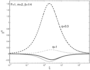
(a) Variation of $\Xi^{A}$ versus $\xi$

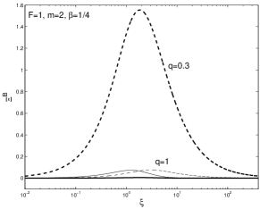
(b) Variation of $\Xi^{B}$ versus $\xi$

Figure 8: Variations of $\Xi^{A}$ and $\Xi^{B}$ versus $\xi$ for the two branches of $y=D^{2}$ solution with $m=2$, $\beta=1/4$, ${F}=1$, and $q=0.3,\ 1$. Solid and dashed curves stand for $y_{1}$ and $y_{2}$ branches, respectively, with heavy and light curves for $q=0.3$ and $q=1$, respectively. Note that $\Xi^{A}$ is positive and negative for $y_{2}$ and $y_{1}$ branches, respectively, while $\Xi^{B}$ is positive for both $y=D^{2}$ branches.

Meanwhile, we compute the other two perturbation contributions to the angular momentum flux, namely, those from the advective transfer and the magnetic torque. For the part of advective transport, we start from equation (85) and make use of phase relationship (80) to explicitly derive

$$\begin{split}&\Re(u_{1})=\frac{m\Omega\sigma\Re(\Theta_{S})}{\Sigma_{0}}r^{-1/2}\sin(\xi\ln r-m\theta)+\frac{m\Omega\sigma\Im(\Theta_{S})}{\Sigma_{0}}r^{-1/2}\cos(\xi\ln r-m\theta)\ ,\\ &\Re(j_{1}/r)=-(\Omega\sigma/\Sigma_{0})[1-(1/2+\beta)\Re(\Theta_{S})-\xi\Im(\Theta_{S})]r^{-1/2}\cos(\xi\ln r-m\theta)\\ &\qquad\qquad\qquad\qquad\qquad\qquad\qquad\ -(\Omega\sigma/\Sigma_{0})[(1/2+\beta)\Im(\Theta_{S})-\xi\Re(\Theta_{S})]r^{-1/2}\sin(\xi\ln r-m\theta)\ .\end{split}$$ (111)

It immediately follows that the advective torque is given by

$$\Lambda^{A}=r^{2}\Sigma_{0}\int_{0}^{2\pi}d\theta\Re(u_{1})\Re(j_{1}/r)=\frac{m\pi\sigma^{2}\Omega^{2}r}{\Sigma_{0}}[\xi|\Theta_{S}|^{2}-\Im(\Theta_{S})]=m\pi^{2}G\sigma^{2}\Xi^{A}\ ,$$ (112)

where

$$\Xi^{A}\equiv\frac{2D^{2}(1+2\beta)[\xi|\Theta_{S}|^{2}-\Im(\Theta_{S})]}{{F}{\cal C}[1+D^{2}-(1-4\beta)q^{2}/(2+4\beta)]}\ ,$$

that is independent of radius $r$. By specifying parameters $\beta$, $m$, ${F}$, $q$ and $\xi$, one finds that for the $y_{1}$ branch $\xi|\Theta_{S}|^{2}-\Im(\Theta_{S})<0$ for $\xi>0$ and $\xi|\Theta_{S}|^{2}-\Im(\Theta_{S})>0$ for $\xi<0$. Therefore, the advective angular momentum flux is radially inward for leading stationary spiral density waves and radially outward for trailing stationary spiral density waves for the $y_{1}$ branch of $D^{2}$ solutions. For the $y_{2}$ branch in comparison, the situation switches and the advective angular momentum flux is outward for leading stationary spiral density waves and inward for trailing stationary spiral density waves. Practically, to achieve the $y_{2}$ branch of stationary logarithmic spiral configurations requires a much lower $D^{2}$ which would be unusual for real magnetized disc systems. An example of illustration for $m=2$, ${F}=1$ and $\beta=1/4$ is shown in panel (a) of Fig. C2.

For the momentum flux associated with the magnetic torque, we start from equation (87) and make use of phase relationship (80) to first derive

$$\begin{split}&\Re(b_{r})=[mB_{0}\sigma\Re(\Theta_{S})/\Sigma_{0}]\ r^{-3/2}\sin(\xi\ln r-m\theta)+[mB_{0}\sigma\Im(\Theta_{S})/\Sigma_{0}]\ r^{-3/2}\cos(\xi\ln r-m\theta)\ ,\\ &\Re(b_{\theta})=[\xi B_{0}\sigma\Re(\Theta_{S})/\Sigma_{0}]\ r^{-3/2}\sin(\xi\ln r-m\theta)+[\xi B_{0}\sigma\Im(\Theta_{S})/\Sigma_{0}]\ r^{-3/2}\cos(\xi\ln r-m\theta)\ .\end{split}$$ (113)

It immediately follows that the momentum flux $\Lambda^{B}$ associated with the magnetic torque is given by

$$\Lambda^{B}=-\frac{r^{2}}{4\pi}\int_{0}^{2\pi}d\theta\int_{-\infty}^{\infty}dz\Re(b_{r})\Re(b_{\theta})=-\frac{m\pi\xi\sigma^{2}C_{A}^{2}|\Theta_{S}|^{2}}{\Sigma_{0}r}=-m\pi^{2}G\sigma^{2}\Xi^{B}\ ,$$ (114)

where

$$\Xi^{B}\equiv\frac{2q^{2}\xi|\Theta_{S}|^{2}}{{F}{\cal C}[1+D^{2}-(1-4\beta)q^{2}/(2+4\beta)]}\ ,$$

which is again independent of radius $r$; here, $\Lambda^{B}$ is inward for leading spiral density waves (i.e., $\xi>0$) and outward for trailing spiral density waves (i.e., $\xi<0$). An example of illustration for $m=2$, ${F}=1$ and $\beta=1/4$ is shown in panel (b) of Fig. C2.

By comparing the three contributions to the total angular momentum flux transport, we reach the following conclusions. First, the contribution from the advective transport part tends to be more dominant over those from the magnetic torque and the gravity torque. Secondly, for the $y_{1}$ branch for stationary fast MHD density waves that has a counterpart in the unmagnetized case, leading spiral density waves ($\xi>0$) transport angular momentum inward and trailing spiral density waves ($\xi<0$) transport angular momentum outward. Thirdly, for the $y_{2}$ branch for stationary slow MHD density waves caused by the very presence of the azimuthal magnetic field, leading spiral density waves ($\xi>0$) carry angular momentum outward and trailing spiral density waves ($\xi<0$) carry angular momentum inward. Note that all these results are only valid for stationary logarithmic spiral MHD density waves. There might be some reasons to rule out the $y_{2}$ branch in galactic contexts. For example, the $y_{2}$ branch is of lower $D^{2}$ which cannot be sustained in real galactic discs. Furthermore, for rotation curve parameter $\beta\neq 1/4$, the $y_{2}$ branch may be ruled out by inequality (17).

References

- [1] Balbus S. A., Hawley J. F., 1998, Rev. Mod. Phys., 70, 1
- [2] Beck R., Brandenburg A., Moss D., Shukurov A., Sokoloff D., 1996, ARA&A, 34, 155
- [3] Beck R., Hoernes P., 1996, Nat, 379, 47
- [4] Binney J., Tremaine S., 1987, Galactic Dynamics. Princeton University Press, Princeton, New Jersey
- [5] Caunt S. E., Tagger M., 2001, A&A, 367, 1095
- [6] Chandrasekhar S., 1961, Hydrodynamic and Hydromagnetic Stability. Dover, New York
- [7] Elmegreen B. G., 1995, MNRAS, 275, 944
- [8] Evans N. W., Read J. C. A., 1998a, MNRAS, 300, 83
- [9] Evans N. W., Read J. C. A., 1998b, MNRAS, 300, 106
- [10] Fan Z. H., Lou Y.-Q., 1996, Nat, 383, 800
- [11] Fan Z. H., Lou Y.-Q., 1999, MNRAS, 307, 645
- [12] Ferrière K. M., 2001, Rev. Mod. Phys., 73, 1031
- [13] Frick P., Beck R., Shukurov A., Sokoloff D., Ehle M., Kamphuis J., 2000, MNRAS, 318, 925
- [14] Frick P., Beck R., Berkhuijsen E. M., Patrickeyev I., 2001, MNRAS, 327, 1145
- [15] Goodman J., Evans N. W., 1999, MNRAS, 309, 599
- [16] Goldreich P., Lynden-Bell D., 1965, MNRAS, 130, 125
- [17] Goldreich P., Tremaine S., 1978, Icarus, 34, 240
- [18] Jog C. J., 1996, MNRAS, 278, 209
- [19] Julian W. H., Toomre A., 1966, ApJ, 146, 810
- [20] Kalnajs A. J., 1971, ApJ, 166, 275
- [21] Kim W.-T., Ostriker E. C., 2000, ApJ, 540, 372
- [22] Kronberg P. P., 1994, Reports on Progress in Physics, 57, 325
- [23] Lemos J. P. S., Kalnajs A. J., Lynden-Bell D., 1991, ApJ, 375, 484
- [24] Lin C. C., Shu F. H., 1964, ApJ, 140, 646
- [25] Lou Y.-Q., 2002, MNRAS, 337, 225
- [26] Lou Y.-Q., Fan Z. H., 1998a, ApJ, 493, 102
- [27] Lou Y.-Q., Fan Z. H., 1998b, MNRAS, 297, 84
- [28] Lou Y.-Q., Fan Z. H., 2000, MNRAS, 315, 646
- [29] Lou Y.-Q., Fan Z. H., 2002, MNRAS, 329, L62
- [30] Lou Y.Q., Walsh W. M., Han J. L., Fan Z. H., 2002, ApJ, 567, 289
- [31] Lou Y. Q., Yuan C., Fan Z. H., 2001, ApJ, 552, 189
- [32] Lou Y. Q., Yuan C., Fan Z. H., Leon S., 2001, ApJ, 553, L35
- [33] Lou Y.-Q., Shen Y., 2003, MNRAS, 343, 750 (astro-ph/0304270)
- [34] Lou Y.-Q., Wu Y., 2004, MNRAS, submitted
- [35] Lou Y.-Q., Zou Y., 2004a, MNRAS, 350, 1220 (astro-ph/0312082)
- [36] Lou Y.-Q., Zou Y., 2004b, MNRAS, submitted
- [37] Low B. C., Lou Y.-Q., 1990, ApJ, 352, 343
- [38] Lynden-Bell D., Kalnajs A. J., 1972, MNRAS, 157, 1
- [39] Lynden-Bell D., Lemos J. P. S., 1993, preprint (astro-ph/9907093)
- [40] Mathewson D. S., van der Kruit P. C., Brouw W. N., 1972, A&A, 17,468
- [41] Mestel L., 1963, MNRAS, 126, 553
- [42] Neininger N., 1992, A&A, 263, 30
- [43] Qian E., 1992, MNRAS, 257, 581
- [44] Rüdiger G., Kitchatinov L. L., 2000, Astro. Nachr., 3, 181
- [45] Safronov V. S., 1960, Ann. Astrophys., 23, 979
- [46] Shakura N. I., Sunyaev R. A., 1973, A&A, 24, 337
- [47] Shen Y., Lou Y.-Q., 2003, MNRAS, 345, 1340 (astro-ph/0308063)
- [48] Shen Y., Lou Y.-Q., 2004a, ChJAA, in press (astro-ph/0404190)
- [49] Shen Y., Lou Y.-Q., 2004b, MNRAS, 353, 249 (astro-ph/0405444)
- [50] Shu F. H., Laughlin G., Lizano S., Galli D., 2000, ApJ, 535, 190
- [51] Shu F. H., Li Z.-Y., 1997, ApJ, 475, 251
- [52] Sofue Y., Fujimoto M., Wielebinski R., 1986, ARA&A, 24, 459
- [53] Spruit H. C., 1987, A&A, 184, 173
- [54] Syer D., Tremaine S., 1996, MNRAS, 281, 925
- [55] Tagger M., Pellat R., 1999, A&A, 349, 1003
- [56] Toomre A., 1964, ApJ, 139, 1217
- [57] Toomre A., 1977, ARA&A, 15, 437
- [58] Visser H. C. D., 1980a, A&A, 88, 149
- [59] Visser H. C. D., 1980b, A&A, 88, 159
- [60] Widrow L. M., 2002, Rev. Mod. Phys., 74, 775
- [61] Zang T. A., 1976, PhD thesis, MIT, Cambridge MA