A High Galactic Latitude HI 21cm-line Absorption Survey using the GMRT: II. Results and Interpretation

Abstract

We have carried out a sensitive high-latitude ($|b|$ $>$ 15^∘) HI 21cm-line absorption survey towards 102 sources using the GMRT. With a $3\sigma$ detection limit in optical depth of $\sim$0.01, this is the most sensitive HI absorption survey. We detected 126 absorption features most of which also have corresponding HI emission features in the Leiden Dwingeloo Survey of Galactic neutral Hydrogen. The histogram of random velocities of the absorption features is well-fit by two Gaussians centered at V_lsr $\sim$ 0 km s^-1 with velocity dispersions of 7.6 $\pm$ 0.3 km s^-1 and 21 $\pm$ 4 km s^-1 respectively. About 20% of the HI absorption features form the larger velocity dispersion component. The HI absorption features forming the narrow Gaussian have a mean optical depth of 0.20 $\pm$ 0.19, a mean HI column density of (1.46 $\pm$ 1.03) $\times$ 10²⁰ cm^-2, and a mean spin temperature of 121 $\pm$ 69 K. These HI concentrations can be identified with the standard HI clouds in the cold neutral medium of the Galaxy. The HI absorption features forming the wider Gaussian have a mean optical depth of 0.04 $\pm$ 0.02, a mean HI column density of (4.3 $\pm$ 3.4) $\times$ 10¹⁹ cm^-2, and a mean spin temperature of 125 $\pm$ 82 K. The HI column densities of these fast clouds decrease with their increasing random velocities. These fast clouds can be identified with a population of clouds detected so far only in optical absorption and in HI emission lines with a similar velocity dispersion. This population of fast clouds is likely to be in the lower Galactic Halo.

1 Introduction

A number of HI 21cm-line absorption surveys have been carried out in the last 50 years or so. While interferometric surveys are a better alternative for such studies, since it rejects the more extended HI emission, the lack of collecting area of the interferometers has limited the sensitivity of the HI absorption surveys. Until recently, the Very Large Array (VLA) used to be the only instrument with a collecting area comparable to large single dish telescopes. From the various HI absorption surveys carried out so far, more than 600 absorption spectra are available, but the optical depth detection limits of more than 75% of these are above 0.1 (see for eg. Mohan et al, 2004 - hereafter paper I, for a summary of previous surveys).

The motivation for the present survey, the observing strategy, the sources observed, their HI 21cm line spectra and the parameters of the discrete HI line components are presented in paper I. Here, we discuss their interpretation. As was mentioned in paper I, the low optical depth regime of Galactic HI is largely unexplored, except for the HI absorption study by Dickey et al (1978) and by Heiles & Troland (2003a, b). Dickey et al. (1978) measured HI absorption/emission towards 27 extragalactic radio sources located at high and intermediate Galactic latitudes ($|b|$ $>$ 5^∘) using the Arecibo telescope. The rms optical depth in their spectra was $\sim$0.005. These profiles can be considered the best in terms of signal-to-noise ratio, though in many of the profiles the systematics in the band dominate the noise. Despite these limitations, Dickey et al (1978) noted that the velocity distribution of HI absorption features is dependent on their optical depths. For the optically thin clouds ($\tau$ $<$ 0.1), the velocity dispersion was $\sim$11 km s^-1, whereas for the optically thick clouds ($\tau$ $>$ 0.1) this value was $\sim$6 km s^-1. Similar trend was also noticed in the Effelsberg-Green Bank survey (Mebold et al, 1982). More recently, Heiles & Troland (2003b) also found indications for an independent population of lower optical depth HI absorption features.

One of the first efforts to study the nature of the ISM was the observation of interstellar absorption in the optical line of singly ionized calcium (CaII) towards early type stars by Adams (1949). He noted that the observed extent in the radial velocities exceeded 50 km s^-1 in the local standard of rest frame (LSR). Blaauw (1952) analysed the random velocity distribution of interstellar absorption lines in Adams’ data. One of the main conclusions of this analysis was that the random velocity distribution of interstellar absorption features cannot be explained by a single Gaussian distribution. Support for this conclusion came from the study of Routly & Spitzer (1952), who found the ratios of column densities of neutral sodium (NaI) to singly ionized calcium (CaI) to decrease systematically with increasing random velocities of the absorption features. This effect, called the “Routly-Spitzer effect” was later confirmed from a much larger sample of stars by Siluk & Silk (1974). Field, Goldsmith & Habbing (1969) modeled the ISM as cool dense concentrations of gas, often referred to as “interstellar clouds” (the Cold Neutral Medium or CNM), in pressure equilibrium with a warmer intercloud medium (the Warm Neutral Medium or WNM). While this initial model of the ISM has been refined considerably by later studies, the basic picture of the ISM with cold diffuse clouds and the warmer intercloud medium has remained. However, there has been a discrepancy in the velocity distribution of interstellar clouds (the CNM) obtained from the optical absorption line studies and from the HI 21-cm line observations. The optical as well as UV absorption line studies indicated the presence of features with larger spread in random velocities, which was absent in the 21-cm line observations (Mohan et al, 2001 & the references therein). This is clear from Fig. 1.

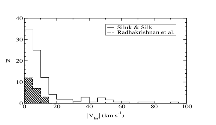
Figure 1: Histogram of radial (random) velocities from the optical absorption line studies by Siluk & Silk (1974), along with that from the HI absorption line survey by Radhakrishnan et al., 1972 (dashed line; shaded). The higher velocity tail is missing in the radio observations.

According to one hypothesis, the high velocity ($|v|$ $\stackrel{{\scriptstyle>}}{{{}_{\sim}}}$ 15 km s^-1) optical absorption lines arise in interstellar clouds, shocked and accelerated by supernova remnants in their late phases of evolution (Siluk & Silk, 1974; Radhakrishnan & Srinivasan, 1980). Such a mechanism would naturally result in the higher random velocity clouds being warmer and having lower column densities due to shock heating and evaporation, as compared to the low random velocity clouds. Lower column density explains the non detections of such clouds in HI emission, since the intensity of the HI 21cm line emission is directly proportional to the HI column density. Higher temperature, along with lower column density ($N_{\scriptscriptstyle{\rm{HI}}}$) results in lower optical depth, since $\tau_{\scriptscriptstyle{\rm{HI}}}$ $\propto$ $N_{{\scriptscriptstyle{\rm{HI}}}}/T$, where $T$ is the excitation temperature of the spectral line (Siluk & Silk, 1974; Radhakrishnan & Srinivasan, 1980; Rajagopal et al, 1998). If this scenario is correct, then a sensitive HI absorption survey should detect those features with lower optical depth and higher random velocities which are presumably the counterparts of the higher velocity optical absorption lines. We have used the present dataset to address this scenario.

In the next section we discuss a method to estimate the contributions from the Galactic differential rotation to the observed radial velocities of the HI absorption features. To supplement the absorption spectra, the corresponding HI 21cm emission profiles from the Leiden-Dwingeloo HI emission survey (LDS, Hartman & Burton, 1995) were analyzed. Appendices B & C of paper I list the HI line profiles (absorption & emission), and their fitted line parameters respectively. In section 3, we compare the present dataset with the previous HI absorption surveys. In Section 4, we discuss the statistics of HI absorption line parameters obtained from the GMRT. The velocity dispersion of the interstellar clouds estimated from the present survey and the low optical depth features are highlighted. In section 5, we compare our results with various other existing studies to discuss the location of the newly detected high random velocity and low optical depth features.

2 The differential Galactic rotation

As was discussed in paper I, we carried out a survey at higher Galactic latitudes to avoid the blending of components in the absorption spectra and to minimize the contribution of the systematic velocities in the observed radial velocities due to the Galaxy’s differential rotation. For a given Galactic longitude ($l$) and latitude ($b$), the observed radial component of differential Galactic rotation for objects in the solar neighbourhood is (Burton, 1988)

$${\rm{v}}_{\scriptscriptstyle{\rm{r}}}=Ar~{}sin~{}2l~{}~{}cos~{}b$$ (1)

where, $A$ = 14 km s^-1 Kpc^-1 is the Oort’s constant and $r$ is the heliocentric distance to the object.

In figure 2 we have plotted the radial velocities with respect to the local standard of rest (LSR) of the various HI absorption features as a function of the Galactic longitude. If the contribution to radial velocities from the Galactic differential rotation is dominant, there should be a pronounced signature of a “sine wave” in such a plot, provided the absorption features are at the same heliocentric distance $r$ (Eqn. 1). There is a suggestion that absorption features with $|V_{lsr}|$ $\stackrel{{\scriptstyle<}}{{{}_{\sim}}}$ 15 km s^-1 may have significant contribution from differential rotation.

Figure 2: The radial velocities (in the LSR frame) of the HI absorption features detected in the present survey as a function of Galactic longitude

Including an additional term for the random motion of the cloud, equation 1 becomes,

$${\rm{v}}_{\scriptscriptstyle{\rm{r}}}={\rm{v}}_{\scriptscriptstyle{\rm{random}}}~{}+~{}Ar~{}sin~{}2l~{}~{}cos~{}b\\$$ (2)

It would appear that this function can be fitted to the observed distribution (Fig. 2) to estimate the systematic component. However, the distances to the absorbing features are unknown. Consider an ensemble of interstellar clouds, each with its own random motion and distance. The random motions can be approximated by a Gaussian with a zero mean. If we assume the number density of clouds to be only a function of height, $|z|$, from the Galactic plane and the Sun to be in the plane, the distances for a distribution of clouds in the Galaxy can be assumed to be an exponential deviate with a scale height (Dickey & Lockman, 1990). Adding these two terms, the above equation can be re-written as

$${\rm{v}}_{\scriptscriptstyle{\rm{r}}}=a_{\scriptscriptstyle{\rm{1}}}{\rm{v}}_{\scriptscriptstyle{\rm{gauss}}}~{}+~{}a_{\scriptscriptstyle{\rm{2}}}\left(\frac{z_{\scriptscriptstyle{\rm{exp}}}}{|sin~{}b|}\right)~{}sin~{}2l~{}~{}cos~{}b\\$$ (3)

Where $z_{\scriptscriptstyle{\rm{exp}}}$ is an Exponential deviate with unit scale height and ${\rm{v}}_{\scriptscriptstyle{\rm{gauss}}}$ is a Gaussian deviate. The term $z_{\scriptscriptstyle{\rm{exp}}}/|sin~{}b|$ is to take into account the variation of path length through the disk as a function of the Galactic latitude. We have carried out a Monte-Carlo simulation to generate such a distribution and compare with the observed distribution (Fig. 2). The simulation used the Monte Carlo routines discussed by Press et al (1992).

We used the $F-test$ (Press et al, 1992) to check if the simulated and the observed data can be derived from the same distribution. We found no well defined peak for the probability distribution. The 3$\sigma$ level indicates that similar confidence levels can be achieved even with $a_{1}$ or $a_{2}$ = 0.0. Therefore, the $F-test$ results imply that a systematic pattern in the distribution is negligible (For a detailed discussion see Mohan, 2003). Hence, we have not applied any correction to the observed velocity for differential Galactic rotation. The observed radial velocities are considered to be random motions. A similar conclusion was also reached by Heiles & Troland (2003b) for the recent Arecibo survey of HI absorption/emission measurements for Galactic latitudes $|b|$ $>$ 10^∘.

3 Comparison of the GMRT data with the previous HI and optical surveys

In this section we compare the histogram of random velocity distribution obtained from the present survey with those from the previous HI absorption line surveys and optical absorption line surveys of interstellar NaI and CaII. For the case of radio surveys, we have used those lines of sight from the previous surveys with $|b|$ $>$ 15^∘. While comparing our data with the results obtained from optical surveys, we have not put this restriction since the stars observed are located in the solar neighbourhood and the contribution from the differential Galactic rotation (if any) would be negligible. We have, however, carefully analysed the optical surveys to exclude those lines of sight where the velocities of the absorption lines were due to systematic motions.

3.1 Comparison of the GMRT data with the previous HI surveys

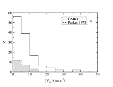
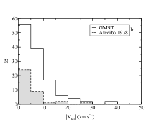
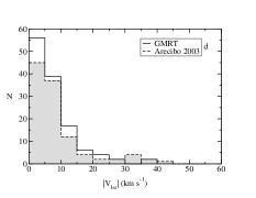
Figure 3: The frequency distribution of mean LSR velocities of the HI absorption features identified from the GMRT survey is compared with that from Radhakrishnan et al (1972) (a), Dickey, Salpeter & Terzian (1978) (b), Mebold et al (1982) (c) and from Heiles & Troland (2003a) (d) respectively.

Figure 3 shows the frequency distribution of radial velocities of HI absorption features from the present survey along with that of 22 HI absorption features from the Parkes Interferometer survey by Radhakrishnan et al (1972), 37 discrete HI absorption features from the Arecibo measurements by Dickey, Salpeter & Terzian (1978) and 51 absorption features from the Effelsberg-Green Bank HI absorption survey by Mebold et al (1981, 1982). No feature at radial velocities larger than 15 km s^-1 was detected in the Parkes survey (Fig. 3a). The Arecibo HI absorption survey by Dickey et al. (1978) had an rms sensitivity comparable to the present survey. Although the number of absorption features from their survey is smaller, the spread in the radial velocities are found to be similar to the present survey. The Effelsberg-Green Bank survey by Mebold et al (1982) lists 69 lines of sight. We have used only the Interferometric measurements from Mebold et al. (1982). Figure 3c shows a comparison of radial velocity histogram from the present survey to that by Mebold et al (1982). It is evident from the figure that except for the single absorption feature at $\sim$35 km s^-1, all the features in the survey by Mebold et al (1982) are at velocities below $\sim$ 20 km s^-1.

It is clear from figures 3a,b &c that the present dataset has not only detected more absorbing clouds, but also more higher velocity clouds. The peak optical depths of these features at higher velocities are found to be lower as compared to the rest of the clouds (See Figure 7). The random velocity distribution of the features detected in the present survey agrees well with that from the recent Arecibo survey by Heiles & Troland (2003a) (Fig. 3d).

There are six common sources between the present survey and the Arecibo observations. While the rms sensitivity in HI optical depth of the Arecibo survey is slightly worse ($\tau_{\scriptscriptstyle{\rm{HI}}}$ $\sim$0.006) compared to the present survey, its velocity resolution (0.16 km s^-1) is better compared to the current HI absorption measurements (3.3 km s^-1). Therefore, the number of HI absorption components detected in their observations are higher than that in the present survey. For the six common sources, the fitted values for the peak optical depths from the present survey and the Arecibo survey agree to within $\sim$ 30%. The fitted values for line centers and widths of the corresponding features differ by less than $\sim$ 2 km s^-1 between the two surveys.

3.2 Comparison of the GMRT HI Absorption data with the Optical surveys

The CaII and NaI absorption studies of Adams (1949), Blaauw (1952), Münch (1957), Münch & Zirin (1961) and others revealed two set of absorption features, one at lower and the other at higher random velocities. More recently, high resolution spectra of NaI lines (eg. Welty et al, 1994) and CaII lines (Welty et al, 1996) were obtained towards a number of stars.

Figure 4a shows the frequency distribution of the velocities of the HI absorption features from the present survey with that from Blaauw’s (1952) study. The secondary peak at high velocity in Blaauw’s histogram is an artifact of the binning used by Blaauw (1952). He counted all the features with radial velocities V_lsr $\geq$ 21 km s^-1 in a single bin. Excluding this secondary peak, there is reasonable agreement between the two histograms.

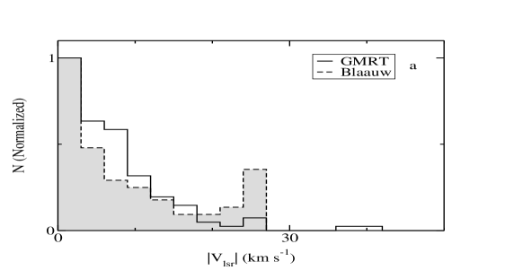
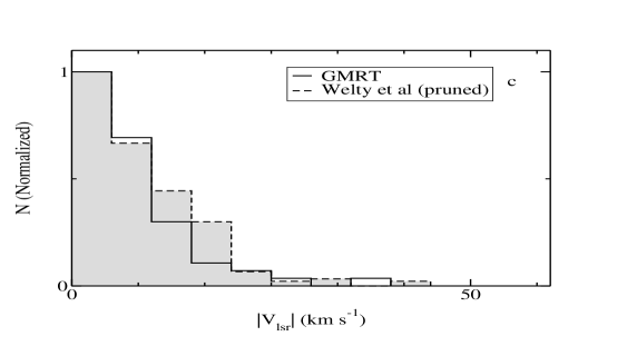
Figure 4: The frequency distribution of the radial velocities of HI absorption features identified from the present survey along with those from optical surveys. (a): Blaauw, 1952 (dashed line). The secondary peak at high velocity in Blaauw’s histogram is an artifact of the binning used by Blaauw. (b): Optical absorption line data from Siluk & Silk, 1974 (pruned), and (c): The CaII absorption survey by Welty, Morton & Hobbs, 1996 (pruned).

In Fig. 4b, we compare the velocity distribution of HI absorption components from the present survey with that from Siluk & Silk (1974). Some of the absorption at higher velocities in their data may not represent random velocities of diffuse HI clouds; they could be due to large systematic motions (Spiral arms, IVCs, HVCs, etc.) superimposed on random motions (Mohan, 2003). Excluding those features, we have re-constructed the histogram of optical absorption line velocities from the data of Siluk & Silk (Fig 4b). The modified histogram from Siluk & Silk (1974) is in good agreement with the current HI absorption velocity histogram.

Fig. 4c compares the frequency distributions of radial velocities from the present survey with that of a recent high resolution survey of CaII lines (Welty et al. 1996). Out of the 44 stars towards which they measured CaII absorption, eight stars were located at a distance of 450 pc, in the constellation Orion, and one star, HD72127, in Vela. The CaII absorption features towards these nine stars were not included in the comparison since the velocities of the absorption features were dominated by systematic motions.

It is clear from figure 4 that the extent of velocities of CaII absorption line features are comparable to that of the HI absorption lines in the present survey. The problem of larger spread in the velocities of interstellar optical absorption lines as compared to the HI 21-cm line features have been an open problem for decades. Our analysis makes it clear that many of the often quoted interstellar optical absorption features at higher velocities may not represent true random motions. Leaving aside such features, the higher velocity HI absorption features detected in the present survey can account for the “missing high random velocity” interstellar clouds in the earlier HI 21-cm line studies.

4 Statistics of the HI absorption line parameters

The details of the observing strategy, the HI absorption spectra from GMRT and the discrete line components identified by fitting Gaussians to the spectra are presented in paper I. Here we discuss their interpretation.

4.1 The frequency distribution of HI absorption line parameters

The frequency distribution of the mean LSR velocities of the HI absorption line components is shown in figure 5a. This histogram was discussed in section 3. It was noticed in earlier studies that the average optical depth of HI absorption features is higher at lower Galactic latitudes (See for eg. Mebold et al., 1982). This apparent excess of large optical depth features in the Galactic plane has been attributed to superposition of absorbing clouds along the line of sight. However, there are only seven features in our survey with their peak optical depths above 0.5 (Fig. 5b). This is an evidence that in the present dataset the superposition of more than one HI absorption feature along the line of sight is minimal. This is expected since we are sampling relatively small path lengths through the gas layer at higher Galactic latitudes.

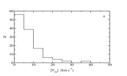
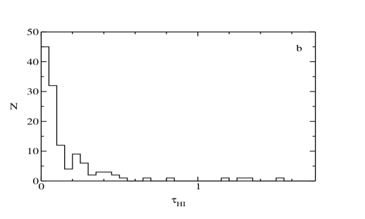
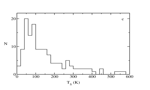
Figure 5: The frequency distribution of the absorption line parameters from the present survey. (a): The histogram of random velocities of the HI absorption components, in 5 km s^-1 bins. (b): The frequency distribution of peak optical depths of HI absorption features, in bins of 0.05 and (c): The frequency distribution of estimated spin temperatures of the HI absorption features in 20 K bins.

As we discussed in paper I, we have used the HI emission data from the Leiden-Dwingeloo survey along with the present GMRT HI absorption data to estimate the spin temperatures of the HI absorption features. The mean value of the spin temperature from the present survey was found to be $\sim$120K, with considerable scatter. For the lower optical depth features ($\tau$ $\stackrel{{\scriptstyle<}}{{{}_{\sim}}}$ 0.1), we find spin temperature, $T_{\scriptscriptstyle{\rm{S}}}$ = 150 $\pm$ 78 K. For the higher optical depth features ($\tau$ $\stackrel{{\scriptstyle>}}{{{}_{\sim}}}$ 0.1), we find $T_{\scriptscriptstyle{\rm{S}}}$ = 74 $\pm$ 30 K. The mean spin temperature of the lower optical depth features, though has a large scatter, is two times higher than that of the higher optical depth features. Figure 5c shows the histogram of the spin temperatures of the HI absorption features. The distribution of spin temperature peaks below 100 K, which agrees in particular with Heiles & Troland (2003b), who found the spin temperature distribution to peak near 40K. Both the Arecibo observations and the present survey indicate the presence of a higher temperature “tail” in the spin temperature histogram.

4.2 The $\tau-$ T_S relation

Several studies in the past had reckoned an inverse correlation between log(1 - e^-τ) and log(T_S) (Lazareff, 1975; Dickey et al., 1979; Crovisier 1981). It was noted that a relationship of the form

$$log\-T_{\scriptscriptstyle{\rm{S}}}=log\-T_{\scriptscriptstyle{\rm{S}0}}+A\-log(1-e^{-\tau})$$ (4)

exists between the observed optical depth and the estimated spin temperature. However, Mebold et al (1982) found no significant correlation between the spin temperature and optical depth. Figure 6 is a plot of (1 - e^-τ) $v/s$ (T_S) from the present dataset. We do find an inverse correlation, though the scatter is larger at lower optical depths. A least square fit to the present dataset provides $T_{\scriptscriptstyle{\rm{S}0}}$ = 43K and $A$ = –0.31 (eqn 4). The values obtained from the previous studies were $\sim$60K and –0.35 respectively (Kulkarni & Heiles, 1988). A similar least-squares fit to the recent Arecibo data yields $A$ = – 0.29 and T_S0 = 33K. However, Heiles & Troland (2003b) have carried out a detailed analysis of the correlation between the various parameters like the spin temperature, the HI column density, the optical depth and the kinetic temperature of the absorption features detected in the Arecibo survey. They emphasize that the mutual correlation that exists between the four parameters renders meaningless the results of least-square fit carried out on only selected pairs of variables. They conclude that there is no physically significant relation between optical depth, spin temperature and HI column density.

Figure 6: log(1 - e^-τ) $-$ log(T_S) plot for the HI absorption features detected in the present survey. HI emission data are from the Leiden-Dwingeloo survey. The dotted line is the best fit for the observed data points. The circles with crosses inside them correspond to the high random velocity HI absorption features (Table 1).

4.3 The $\tau_{\scriptscriptstyle{\rm{HI}}}$ $-$ V_LSR relation

The peak optical depth as a function of $|V_{\scriptscriptstyle{\rm{LSR}}}|$ is shown in figure 7. The peak $\tau_{\scriptscriptstyle{\rm{HI}}}$ drops sharply near $|V_{\scriptscriptstyle{\rm{lsr}}}|$ $\sim$ 10 km s^-1. No spectral features at velocities above 10 km s^-1 have peak optical depth above $\sim$ 0.1. On the other hand, low optical depth features are detected over a larger velocity range. In section 4.1 we found that lower optical depth features have higher mean spin temperature, almost a factor of two higher than the higher optical depth features. Fig. 7 conveys an extra information that these higher spin temperature features are also spread over a larger range in random velocity.

Figure 7: $\tau_{\scriptscriptstyle{\rm{HI}}}$ $-$ $|V_{\scriptscriptstyle{\rm{LSR}}}|$ plot. The higher optical depth features are confined to $|V_{\scriptscriptstyle{\rm{LSR}}}|$ $\stackrel{{\scriptstyle<}}{{{}_{\sim}}}$ 15 km s^-1.

4.4 The distribution of the HI optical depth as a function of $b$

Figure 8: The distribution of optical depth of the HI absorption line features as a function of Galactic latitude. The number of higher optical depth features drop gradually with increasing latitude, but the number of low optical depth features ($\tau$ $\stackrel{{\scriptstyle<}}{{{}_{\sim}}}$ 0.1) remain more or less the same.

HI optical depth of the absorption features are plotted against their Galactic latitude in Figure 8. The optically thick components ($\tau$ $>$ 1.0), though very few, are all confined to $|b|$ $\stackrel{{\scriptstyle<}}{{{}_{\sim}}}$ 30^∘. The low optical depth features ($\tau$ $\stackrel{{\scriptstyle<}}{{{}_{\sim}}}$ 0.1), on the other hand, are almost uniformly distributed with respect to the Galactic latitude. This is an indication that the scale height of the low optical depth features are different from that of the higher optical depth features.

4.5 The velocity dispersion of interstellar Clouds

The velocity distribution of cold atomic gas in the Galaxy is known to be a Gaussian with a dispersion of $\sim$7 km s^-1 (Dickey & Lockman, 1990). As we concluded in section 2, the observed radial velocities of the HI absorption components detected in the present survey are essentially random velocities. We have carried out a Gaussian fit to the observed frequency distribution of the radial velocities of the HI absorption features detected in the present study (Fig. 9). A non-linear least square method was used to fit Gaussians to this histogram. A two Gaussian model was found to be a good fit for the distribution, with a reduced chi-square value of 1.4. The low velocity features were found to form a Gaussian distribution with a velocity dispersion of $\sigma_{1}$ = 7.6 $\pm$ 0.3 km s^-1, which agrees well with the earlier results. For eg., Belfort & Crovisier (1984) had performed a statistical analysis of the radial velocities of HI clouds observed by surveys using the Arecibo (Dickey et al, 1978), and Effelsberg & Green Bank (Mebold et al, 1982). Their value for the velocity dispersion of HI clouds was $\sim$6.9 km s^-1. The higher velocity features in the present survey seem to form a distribution with a velocity dispersion of $\sigma_{2}$ = 21 $\pm$ 4 km s^-1 (Fig. 9). The presence of two Gaussian features in the velocity distribution of interstellar clouds is indicative of two distinct populations of interstellar clouds. From the area under the respective curves, this data indicates that $\sim$20% of the clouds belong to the second population, with larger velocity dispersion.

Figure 9: The frequency distribution of LSR (random) velocities of HI absorption components from the present survey. The dashed line is the sum of two Gaussian components with $\sigma_{1}$ = 7.6 $\pm$ 0.3 km s^-1 and $\sigma_{2}$ = 21 $\pm$ 4 km s^-1. Both the Gaussians are centered at v_LSR = 0 km s^-1. The lower panel shows the residual after subtracting the fitted model from the observed distribution.

A study of the velocities of interstellar optical absorption lines (NaI & CaII) were carried out by Sembach & Danks (1994). They observed that only a two component model can be fitted to the velocity distribution of CaII line components. The values which they obtained were: $\sigma_{1}$ $\sim$8 km s^-1 and $\sigma_{2}$ $\sim$21 km s^-1, which agree well with the velocity dispersions of the two components obtained from the present data of HI absorption lines.

4.6 The High velocity HI absorption features

We have detected 13 HI absorption features at higher random velocities ($|v|$ $>$ 15 km s^-1), out of the 126 total HI absorption features (Table 1). The optical depths of these higher velocity features are below 0.1. The mean value of peak optical depth of all these features is 0.04 $\pm$ 0.02. In most cases, we could identify the corresponding HI emission feature in the HI emission profile from the Leiden-Dwingeloo survey. If the velocity difference between the absorption and the emission line was less than or comparable to the channel width of the GMRT observations ($\sim$3.3 km s^-1), and if the difference between line widths was within $\sim$ 5 km s^-1, the spectral lines were assumed to originate in the same physical feature. The mean brightness temperature of these features was $\sim$4 K and a mean HI column density of (4.3 $\pm$ 3.4) $\times$ 10¹⁹ cm^-2. The mean value of the spin temperatures of these clouds is 125 $\pm$ 82 K.

Table 1: The higher random velocity ($|v|$ $\stackrel{{\scriptstyle>}}{{{}_{\sim}}}$ 15 km s^-1) HI absorption features detected in the present survey. Columns 2, 3 and 4 list the peak optical depth, the mean LSR velocity and the FWHM respectively of discrete components identified using the Gaussian fitting. The value of FWHM is deconvolved for a channel width of 3.26 km s^-1. The unresolved lines are marked with a ”–” . Columns 5, 6 and 7 list the same for the HI emission profile along the same line of sight, obtained from the Leiden-Dwingeloo survey of Galactic neutral hydrogen (Hartman & Burton, 1995) The formal 1$\sigma$ errors estimated in the last digit of the fitted parameters are given within brackets. The implied HI column densities are listed in column 8 and the estimated spin temperatures are given in column 9.

	HI Absorption (GMRT)				HI Emission (LDS)
Source	$\tau_{\scriptscriptstyle{\rm{HI}}}$	vlsr	$\Delta$v		TB	vlsr	$\Delta$v	NHI	TS
								$\times$ 1019
		(km/s)	(km/s)		(K)	(km/s)	(km/s)	cm-2	(K)
J0459+024	0.026(4)	–25.6(5)	4.6(8)		0.21(8)	–28(1)	6(3)	0.24	8
J0541–056	0.069(7)	+17.8(9)	3.2(5)		—	—	—	—
J0814+459	0.035(2)	+16.8(9)	4(2)		9.5(5)	+15.4(1)	3.8(1)	7.0	276
J1154–350	0.016(3)	–16(2)	13(5)		—	—	—	—
J1221+282	$\sim$0.01	–20	–		0.47(4)	–18.9(4)	11(1)	1.0	47
	$\sim$0.02	–38	–		1.06(4)	–34.8(1)	6.1(3)	1.2	53
J1257–319	0.108(6)	–16.0(2)	3.8(3)		—	—	—	—
J1351–148	0.020(4)	+22.0(6)	5(1)		5.7(1)	+22.9(1)	10.5(2)	12.0	285
J1554–270	0.04(2)	–16(8)	8(5)		—	—	—	—
J1638+625	0.028(4)	–20.1(4)	5(1)		4.50(6)	–21.05(2)	5.05(7)	4.4	161
J1751+096	0.066(3)	+25.6(2)	4.6(2)		3.9(1)	+25.1(1)	7.1(3)	5.3	61
J2005+778	0.05(1)	–25(4)	2(2)		7.2(3)	–23.59(8)	7.4(2)	10.0	148
J2232+117	0.040(4)	–15.3(3)	2.9(7)		3.83(7)	–13.88(3)	3.92(8)	2.3	96

We analysed the HI emission profiles from the Leiden-Dwingeloo survey towards 91 directions along which we measured HI absorption using the GMRT. HI column density of individual features along these directions were calculated using the emission data. However, 11 out of the 102 directions studied using the GMRT were beyond the declination limit of the Leiden-Dwingeloo survey. Towards these sources we assumed a spin temperature of 120 K and the observed widths of the HI absorption lines to estimate the column density.

Figure 10: The column densities of the HI absorption features detected in the present survey. The brightness temperature and line width of the HI emission feature corresponding to each absorption feature was obtained from the Leiden-Dwingeloo survey. For those directions where HI emission data is not available, we have assumed a spin temperature of 120K and the velocity width of the HI absorption line to calculate the column density. The squares are the HI column density estimates from the UV absorption line data from Martin and York (1982). and the arrows are the upper limits.

The estimated HI column density as a function of the LSR velocity is shown in fig. 10. The measured HI column density ranges from $\sim$2.4 $\times$ 10¹⁸ to $\sim$9 $\times$ ²⁰ cm^-2. It is clear from fig. 10 that the column densities of the features are decreasing systematically with increasing velocity. This is in agreement with the results from UV absorption line studies (Martin & York, 1982; Hobbs, 1984).

5 Discussion

The present high-latitude, high-sensitivity HI absorption survey from the GMRT has confirmed many of the known results. These results are summarised in the histograms (Fig. 5) of random velocity, peak optical depth, and spin temperature of the absorption components. In addition, variation of peak optical depth w.r.t. spin temperature, random velocity and Galactic latitude are displayed in Figs. 6, 7 and 8 respectively. However, a completely new result is the detection of the low optical depth absorption features forming the high velocity tail in the histogram shown in Fig. 5a. Most of these low optical depth features are below the detection limit of the earlier HI absorption surveys. The velocity histogram (Fig. 5a) is well-fit by two Gaussians indicating two populations of HI absorbing clouds identified by velocity dispersions $\sim$ 7 and $\sim$ 21 km s^-1 respectively (Fig. 9). While the slow clouds were first detected in the optical absorption lines and subsequently in the HI absorption and emission surveys, the fast clouds were only detected in optical absorption lines. The non-detection of the fast clouds remained a puzzle for a long time. The present observations have clarified the nature of the fast clouds to some extent.

There have been attempts in the past to explain the high velocity tail seen in the histogram of random velocities of the optical absorption lines ( Siluk & Silk (1974), Radhakrishnan & Srinivasan (1980), Rajagopal et al (1998)). According to these authors, the high velocity optical absorption lines arise in interstellar clouds, shocked and accelerated by supernova remnants in their late phases of evolution. The fast clouds are therefore warmer and also of lower HI column density as compared to the slow clouds, due to shock heating and evaporation. The present observations indicate that these fast clouds have three times larger velocity dispersion and ten times lower column densities compared to the slow clouds as might be expected if they were from a shocked population of clouds. The decrease in the HI column densities of the fast clouds as a function of their random velocities (Fig. 10) is also consistent with this scenario. The shocked HI clouds are also expected to be warmer than the slow clouds. The mean spin temperature of the fast clouds detected in the GMRT survey is similar to that of the standard slow clouds (Fig. 6). However, this might be a selection effect since for a given optical depth detection limit and an HI column density, clouds with lower spin temperature will be preferentially detected.

The fast clouds with three times higher dispersion are expected to have a scale height about ten times larger compared to the slow HI clouds. Given an effective thickness of 250 pc for the slow clouds, the fast clouds can have an effective thickness of $\sim$ 2.5 kpc. Therefore, fast clouds can be part of the halo of the Galaxy. Alternative evidence supports the existence of atomic gas in the Galactic halo. Albert (1983) selected lines of sight wherein a halo star and a nearby star are aligned one behind the other. Absorption lines of TiII, CaII and NaI were measured towards these stars. Though with a limited sample size of nine directions, the results of this study clearly indicate that the higher velocity absorption lines are seen only towards the distant star. She concludes that the high velocity tail seen in the optical line studies arise from the gas in the Galactic halo. Later, similar studies (Danly, 1989; Danly et al, 1992; Albert et al, 1994; Kennedy et al, 1996, 1998a, 1998b) confirmed this result. The halo gas shows a larger spread in velocity, as compared to the gas in the Galactic disk. Furthermore, recent HI emission studies using the Green Bank telescope have led to the discovery of a population of discrete HI clouds in the Galactic halo with a velocity dispersion similar to that of the fast clouds reported here (Lockman 2002). The mean HI column density of these clouds was estimated to be a few times 10¹⁹ cm^-2. He concludes that a cloud population with a line of sight velocity dispersions of $\sigma_{v}$ $\sim$15 – 20 km s^-1 is capable of explaining the observed velocity spread of these features. Lockman (2002) finds that many clouds in the halo have narrow line widths implying temperatures below 1000K. In addition, indications for a core-halo structure for these clouds was also found. The fast clouds detected in the present survey are likely to be part of the same halo gas detected in HI emission from Green Bank. The fast clouds, once detected only in optical absorption lines, have now been detected in both HI absorption and emission leading to a clearer picture of the interstellar medium.

Acknowledgements:
We wish to thank Shiv Sethi for useful discussions related to the numerical techniques. We thank the referee, Miller Goss, for detailed comments and constructive criticisms resulting in an improved version of this paper. We thank the staff of the GMRT who made these observations possible. The GMRT is operated by the National Centre for Radio Astrophysics of the Tata Institute of Fundamental Research. This research has made use of NASA’s Astrophysics Data System.

References

- [1] Albert, C.E., 1983, Astrophys. J., 272, 509.
- [2] Albert, C.E., Welsh, B.Y., Danly, L., 1994, Astrophys. J., 437, 204.
- [3] Adams, W. A., 1949, Astrophys. J., 109, 354.
- [4] Belfort, P., Crovisier, J., 1984, Astron. Astrophys., 136, 368.
- [5] Blaauw, A., 1952, Bull. Astr. Inst. Netherland., 11, 459.
- [6] Burton, W.B., 1988, in Galactic and Extragalactic Radio Astronomy, eds. G.L. Verschuur & K.I. Kellermann (New York: Springer-Verlag), 295.
- [7] Crovisier, J., 1981, Astron. Astrophys., 94, 162.
- [8] Danly, L., 1989, Astrophys. J., 342, 785.
- [9] Danly, L., Lockman, F.J., Meade, M.R., Savage, B.D., 1992, Astrophys. J. Suppl., 81, 125.
- [10] Dickey, J.M., Lockman, F.J., 1990, Ann. Rev. Astron. Astrophys., 28, 215.
- [11] Dickey, J.M., Salpeter, E.E., Terzian, Y., 1978, Astrophys. J. Suppl., 36, 77.
- [12] Dickey, J.M., Salpeter, E.E., Terzian, Y., 1979, Astrophys. J., 228, 465.
- [13] Field, G.B., Goldsmith, D.W., Habing, H.J., 1969, Astrophys. J.Lett., 155, L149.
- [14] Hartmann, D., Burton, W. B., 1995, An Atlas of Galactic Neutral Hydrogen, Cambridge Univ. Press.
- [15] Heiles, C., Troland, T. H., 2003a, Astrophys. J. Suppl., 145, 329.
- [16] Heiles, C., Troland, T. H., 2003b, Astrophys. J., 586, 1067.
- [17] Hobbs, L.M., 1984, Astrophys. J. Suppl., 56, 315.
- [18] Kennedy, D.C., Bates, B., Kemp, S.N., 1996, Astron. Astrophys., 309, 109.
- [19] Kennedy, D.C., Bates, B., Keenan, F.P., Kemp, S.N., Ryans, R.S.I., Davies, R.D., Sembach, K.R. 1998a, Mon. not. R. Astron. Soc., 297, 849.
- [20] Kennedy, D.C., Bates, B., Kemp, S.N., 1998b, Astron. Astrophys., 336, 315.
- [21] Kulkarni, S. R., Heiles, C. 1988, in Galactic and Extragalactic Radio Astronomy, eds. G.L. Verschuur & K.I. Kellermann (New York: Springer-Verlag), 95.
- [22] Lazareff, B., 1975, Astron. Astrophys., 42, 25.
- [23] Lockman, F.J., 2002, Astrophys. J. Lett., 580, L47.
- [24] Martin, E.R., York, D.G., 1982, Astrophys. J., 257, 135.
- [25] Mebold, U., Winnberg, A., Kalberla, P.M.W., Goss, W.M., 1981, Astron. Astrophys. Suppl., 46, 389.
- [26] Mebold, U., Winnberg, A., Kalberla, P.M.W., Goss, W.M., 1982, Astron. Astrophys. , 115, 223.
- [27] Mohan, R., Dwarakanath, K.S., Srinivasan, G., Chengalur, J.N., 2001, J. Astrophys. Astron., 22, 35.
- [28] Mohan, R., Ph.D. Thesis., 2003 Jawaharlal Nehru University, New Delhi.
- [29] Mohan, R., Dwarakanath, K.S., Srinivasan, G., 2004 (Paper I), J. Astrophys. Astron., this vol..
- [30] Münch, G., 1957, Astrophys. J., 125, 42.
- [31] Münch, G., Zirrin, H., 1961, Astrophys. J., 133, 11.
- [32] Press, W.H., Teukolsky, S.A., Vetterling, W.T., Flannery, B.P., 1992, Numerical Recipes, The Art of Scientific Computing, Cambridge Univ. Press, Cambridge.
- [33] Radhakrishnan, V., Goss, W.M., Murray, J.D., Brooks, J.W., 1972, Astrophys. J. Suppl., 24, 49.
- [34] Radhakrishnan, V., Srinivasan, G., 1980, J. Astrophys. Astr., 1, 47.
- [35] Rajagopal J., Srinivasan, G., Dwarakanath, K. S., 1998, J. Astrophys. Astr., 19, 117.
- [36] Routly, P. M., Spitzer, L. Jr., 1952, Astrophys. J., 115, 227.
- [37] Sembach, K.R., Danks, A.C., 1994, Astron. Astrophys. , 289, 539.
- [38] Siluk, R.S., Silk, J., 1974, Astrophys. J., 192, 51.
- [39] Welty, D. E., Hobbs, L. M., Kulkarni, V.P., 1994, Astrophys. J., 436, 152.
- [40] Welty, D. E., Morton D. C., Hobbs, L. M., 1996, Astrophys. J.Suppl., 106, 533.