Strategies for Spectral Profile Inversion using Artificial Neural Networks

Abstract

This paper explores three different strategies for the inversion of spectral lines (and their Stokes profiles) using artificial neural networks. It is shown that a straightforward approach in which the network is trained with synthetic spectra from a simplified model leads to considerable errors in the inversion of real observations. This problem can be overcome in at least two different ways that are studied here in detail. The first method makes use of an additional pre-processing auto-associative neural network to project the observed profile into the theoretical model subspace. The second method considers a suitable regularization of the neural network used for the inversion. These new techniques are shown to be robust and reliable when applied to the inversion of both synthetic and observed data, with errors typically below $\sim$100 G.

1 Introduction

The analysis of the spectral properties of the light intensity and its polarization state is the basis of modern solar physics. For over two decades, least-squares profile fitting has been the method of choice (see Socas-Navarro 2001; del Toro Iniesta 2003 and references therein). Many different inversion codes, based on a variety of physical models, have been developed and used extensively for the determination of magnetic and thermodynamic conditions in the atmosphere.

While the use of least-squares fitting has important benefits, there is an increasing demand for alternative procedures that are faster and more robust. By robust I mean capable of operating reliably without human intervention on a routine basis. This demand is driven by the development of a new generation of spectro-polarimeters, which will deliver enormous data flows (SOLIS, Keller 1998; Solar-B, Lites et al. 2001; Sunrise, Schmidt et al. 2003; DLSP, Sankarasubramanian et al. 2003).

The attention of solar physicist has turned in recent years towards a new breed of diagnostic techniques based on pattern recognition and machine learning. A considerable number of papers has been devoted to the investigation of these techniques (Rees et al. 2000; Socas-Navarro et al. 2001; Carroll & Staude 2001; Skumanich & López Ariste 2002; Socas-Navarro 2003; del Toro Iniesta & López Ariste 2003; Socas-Navarro 2004). Most of those works deal with the Principal Component Analysis, which is a series expansion of the spectra. Another line of research explores the use artificial neural networks (ANNs), which show considerable promise for the inversion of spectral observations (Carroll & Staude 2001; Socas-Navarro 2003).

The work presented here demonstrates the applicability of ANNs to actual observed data in typical working conditions. The radiative transfer computations that are needed to synthesize training profiles have been carried out using the Milne-Eddington approximation. This is helpful to simplify the problem and to allow for the synthesis of thousands of profiles in a reasonable computing time. All the calculations done for this work, and the CPU times quoted below, were obtained using a Pentium IV processor running at 1.2 GHz. The ANN inversions require very little computational resolurces both in terms of processor speed and memory storage. The training algorithm, on the other hand, can be very demanding.

2 The neural network

An ANN is a structure of interconnected neurons, where each neuron is a memory cell with the capability to store a real number. The number stored in a neuron can be modified according to the contents of its neighbors and the “synaptic weights” that connect each pair of neurons. A perturbation in the contents of a neuron propagates through the network following the structure of connections and synaptic weights. For a sake of tractability, it is customary to consider forward-propagating networks. These ANNs have a well defined signal propagation direction, starting at a set of input neurons and ending at the outputs. No feed-back loops are allowed in forward-propagating networks.

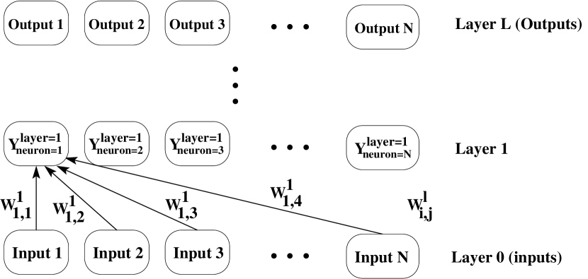
As a further simplification, we shall be concerned only with a particular network configuration: the multilayer perceptron. In this configuration the neurons are arranged in successive layers. Each neuron in any given layer has connections to all neurons in the previous layer. No connections are allowed between non-successive layers. An arbitrary number of intermediate layers may exist between the inputs and outputs. These are usually referred to as “hidden” layers in the ANN literature. A schematic representation of a multi-layer perceptron with hidden layers is given in Fig 1.

Figure 1: Schematic representation of a multi-layer perceptron. Figure reproduced from Socas-Navarro (2004)

When a set of input data is introduced in the ANN, it is propagated forward according to the following rule:

$$Y^{l}_{n}=f_{l}\left(\sum_{j=1}^{N}W^{l}_{n,j}Y^{l-1}_{j}+\beta^{l}_{n}\right)\,.$$ (1)

In Eq (1), $Y^{l}_{n}$ represents the contents of neuron $n$ in layer $l$, $W^{l}_{n,j}$ is the synaptic weight of the connection between this neuron and neuron $j$ in layer $l-1$ and $\beta^{l}_{n}$ is a bias level. We consider the input neurons as layer $l=0$. One or more of the ANN layers may have a non-linear “activation function” $f_{l}(x)$. The ANNs used in this work all have:

$$f_{l}(x) = x\,\,\,{\rm(for\,linear\,layers)}\,,$$

$$f_{l}(x) = a\tanh(bx)\,\,\,{\rm(for\,non-linear\,layers)}\,.$$ (2)

The hyperbolic tangent is a common choice for the non-linear activation function in many ANN applications and has been adopted here for that reason. Other suitable functions are likely to exist, but will not be pursued here. After some experimentation with a simplified problem, the parameters $a$ and $b$ have been set to $1.72$ and $0.67$, respectively.

Conceptually, a multilayer perceptron may be viewed as a non-linear mapping ${\bf F}$ between two multi-dimensional spaces. We can write down:

$${\bf o}={\bf F}({\bf x})\,,$$ (3)

where ${\bf x}$ is an N-dimensional input vector and ${\bf o}$ is an M-dimensional output vector. It can be shown (e.g., Jones 1990; Blum & Li 1991) that a multilayer perceptron with at least one hidden non-linear layer is able to approximate any continuous multidimensional non-linear function to any arbitrary precision, provided only that enough neurons are employed. This is a very interesting mathematical property that has received considerable attention in the ANN literature, since it provides a solid foundation for many applications.

An ANN is fully characterized by its structure and the individual properties of its neurons. The network structure is defined by a set of parameters such as the number of layers $N_{L}$, the number of neurons in a given layer $N_{N}(l)$ (where $l$ denotes the layer), and the activation function of each layer $f_{l}(x)$ which can only be one of the two options given explicitly in Eq (2) above. According to the choice of $f_{l}$ we shall use the terminology of linear/non-linear layers.

The other set of parameters that completely defines an ANN consists of the neural biases and synaptic weights ($\beta^{l}_{n}$ and $W^{l}_{n,j}$ in Eq [1]) for each single neuron.

The most important difference between these two sets of parameters is that the network structure is established a priori for a given problem and then kept fixed throughout. The neuron properties (synaptic weights and biases), however, are adaptive parameters that are continuously adjusted during the ANN training process (described below) to optimize the network performance. Although there are algorithms that modify the network structure during the training process seeking the optimum configuration, I have not made use of such techniques in the present work. The various ANN structures used here are the result of a number of trial-and-error experiments. A detailed study of the impact that the ANN structure has on its performance would be tremendously expensive from a computational point of view due to the long processing times involved in training a single network (typically several days running on a modern workstation).

The ANNs used for the calculations in this work have two linear and two non-linear layers interleaved. All layers, including the inputs, contain the same number of neurons (rectangular ANNs). The exception to this is the AANN of §4 which has a smaller number of neurons in one of the hidden layers.

2.1 Training a network

The previous section described the structure of a typical ANN with particular emphasis on the case of the multilayer perceptron, because this is the type of ANN employed here. However, nothing has been said thus far about the particular values that should be given to $W^{l}_{n,j}$ and $\beta^{l}_{n}$. It is obvious that the behavior of the ANN will be dictated by these parameters, which define the actual mapping ${\bf F}$ performed by the ANN.

The optimal synaptic parameters are obtained by means of a “training” process. For the training we need a large set of input vectors $x^{t}_{i}$ and the solutions or outputs $o^{t}_{j}$ that we wish the ANN to find (for this reason the outputs are sometimes referred to as “targets”). To fix ideas, suppose that we are training an ANN to take a set of observed spectral profiles as inputs and return as outputs some parameters of the atmosphere in which the profiles originated (e.g., temperature, velocity or magnetic field). In this case, the $x^{t}_{i}$ are the observable quantities and the $o^{t}_{j}$ are the atmospheric conditions (in practical situations, one should first pre-process the inputs and outputs as explained below; therefore these parameters are related to the actual physical quantities but they are not the quantities themselves).

It might seem that, in order to generate a suitable training set one needs to invert the $x^{t}_{i}$ in order to produce the $o^{t}_{j}$, which would require the use of some sort of inversion procedure. However, this is not necessarily the case. One could start with the atmospheric parameters (from which the $o^{t}_{j}$ are calculated) and then solve the forward problem to synthesize spectral profiles (thus obtaining the $x^{t}_{i}$).

When the input data are forward-propagated through the ANN we obtain a set of outputs $o_{j}$ which are, in general, different from the targets $o^{t}_{j}$. The training algorithm seeks to minimize the difference between the outputs $o_{j}$ and the targets $o^{t}_{j}$ over the entire training set, e.g. in a least-squares sense by minimizing $\chi^{2}=\sum_{j}(o_{j}-o^{t}_{j})^{2}$. The most widely used procedure to accomplish this task is the back-propagation algorithm, which performs a non-linear least-squares minimization of the distance between the network output and the targets (Rumelhart et al. 1986).

The back-propagation algorithm needs a starting guess for the synaptic parameters. I have found that a random initialization with a normal distribution works well for the applications described here. The amplitude of the distribution is set to 1/$N_{N}(l)$. This is done to ensure that the $Y_{n}^{l}$ are of the order of 1. Otherwise one risks entering the saturation regime of the non-linear activation function. For the same reason it is important to pre-process the inputs and outputs with a linear transformation to bring them within the [-1,1] interval (or at least within that order of magnitude). This has been done here by subtracting the mean value and normalizing to the standard deviation of each parameter over the entire dataset.

For a sake of simplicity, the ANNs used in this work have been trained to retrieve the magnetic field strength only. It is straightforward to train similar networks to retrieve any other model parameters that are deemed relevant. An alternative approach would be to train one single ANN to retrieve all the parameters. Unfortunately, numerical experimentation suggests that a much larger number of neurons is necessary if one wishes to achieve a comparable accuracy in each individual parameter, which increases the computational cost very rapidly. Therefore, it is probably more efficient to train a separate ANN for each parameter. In this manner the computing time for the training and the subsequent inversions scales linearly with the number of parameters. The additional expense for inverting more than one parameter is negligible, considering that a typical inversion such as the ones presented below take only a matter of seconds (compared to several hours for a full Milne-Eddington inversion).

2.2 The training and validation sets

The ANNs are trained in successive epochs. A batch of 15000 profiles are synthesized at each epoch of the training and presented to the network. The use of many batches helps to minimize “overfitting”, which is a common problem encountered in these applications. Overfitting makes an ANN reproduce noise or other irrelevant features of the dataset and lose generalization ability. In fact, accuracy and generalization ability are often opposing atributes and one needs to find an adequate compromise between the two. This is discussed in more detail in the following sections.

The Milne-Eddington approximation is used for all the spectral synthesis calculations in this paper. This approximation considers that all the relevant parameters that enter the radiative transfer equation (magnetic field, line strength, Doppler width, and damping) are constant with height in the line formation region, except for the source function which varies linearly with optical depth (see, e.g., Landi Degl’Innocenti 1992 for details). With these assumptions the solution to the radiative transfer equation is analytical, which alleviates considerably the burden of computing thousands of training spectral line profiles. In addition to these atmospheric parameters I consider a “filling factor” ($\alpha$) of the magnetic element, which is used to treat spatially unresolved fields. The magnetic profile is multiplied by $\alpha$ and added a quiet-Sun profile multiplied by $(1-\alpha)$.

The starting model atmospheres for the spectral syntheses are random but based on a distribution obtained from actual solar data. I have used existing observations in the archives of the Advanced Stokes Polarimeter (ASP, Elmore et al. 1992; Lites 1996) to obtain a realistic distribution of the Milne-Eddington parameters. Histograms of some of the most relevant parameters are shown in Fig 2. The various atmospheric parameters are not independent of one another. Fig 3 shows the correlations existing between some relevant parameters.

Figure 2: Histograms of the distribution of some atmospheric parameters used for the synthesis of training data.

The use of solar distributions has the advantage of optimizing the network performance for the observations that one expects to find in the real Sun (at least in a statistical sense).

Figure 3: Correlations between the magnetic field strength and some other atmospheric parameters used for the synthesis of training data.

The profiles calculated are those of the Fe I pair of lines near 6302 Å. The spectra are sampled in 52 mÅ  bins, about a factor of 4 lower than typical ASP observations. The wavelength range where two telluric lines are present in actual observations is removed from the synthetic profiles.

Once the ANN has been trained, two different tests are used to assess its performance. The first test uses synthetic profiles obtained from a Milne-Eddington inversion of ASP observations. The inversions were carried out by Lites et al. 1998 using the code developed by Skumanich & Lites (1987). The observed region can be considered rather typical and contains significant areas of quiet Sun, a fairly round sunspot and some plage, and has a fairly good spatial resolution ($\simeq$1”) consistently during the entire scan. Fig 4 shows several maps of the observed region.

Figure 4: Observed region. Upper left: Continuum intensity. Upper right: Intrinsic field strength. Lower left: Degree of circular polarization (saturated at $\pm$10%). Lower right: Filling factor of the magnetic element in the pixel ($\alpha$).

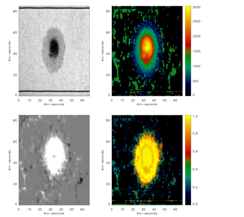
The test with synthetic profiles has the advantage that the sought solution is known beforehand. Both the training and the validation data have been produced using the Milne-Eddington approximation, so the models are consistent physically. Therefore, the errors obtained can be ascribed directly to the ANN performance.

Unfortunately, the performance of an ANN may be very different when it is applied to simplified synthetic profiles or to real observations. It is then crucial to consider a second test in which the validation data are observations. For this purpose I have used the spectral profiles from the ASP dataset described above. The ANN outputs are compared to the models resulting from the Milne-Eddington inversion to estimate the errors.

3 The direct approach

Let us first consider the most straightforward approach, which is to train the ANN with synthetic profiles as explained in §2.2. Each input vector has a total of 80 elements, corresponding to 4 Stokes parameters, 2 spectral lines and 10 spectral samples per line. Output vectors have only 1 element, namely the intrinsic magnetic field strength (see last paragraph of §2.1).

Some basic pre-processing is applied to the synthetic profiles before they are presented to the ANN. This is intended to reduce the dimensionality of the problem by removing trivial transformations. The following procedures are applied:

• The global bulk velocity is removed by shifting all profiles so that their Stokes $I$ “center of symmetry” are at the same position. The center of symmetry is defined so that the sum of quadratic differences of symmetric points in the line profile are minimal.

• Random noise is added to all profiles. The noise has a normal distribution and an amplitude of 10^-3 times the continuum intensity.

• All profiles are normalized to their respective continuum intensity.

• The spectral ranges of the two telluric lines are removed.

• The mean and standard deviation of each spectral sample over the entire training set are computed. These are then used to normalize the inputs so that they are of the order of 1. The same is done for the output magnetic fields.

The ANN is trained in successive epochs with batches of 15000 profiles. For each epoch, the back-propagation algorithm is applied until 500 iterations are performed or the last 50 iterations do not result in further improvement. After a training epoch, the ANN is presented with 500 new profiles that were not included in the training set. This validation set is used to estimate the performance of the network when presented with new data. The training process is repeated in successive training epochs with different sets until the validation error converges (i.e., it no longer decreases with additional training batches).

Figure 5: Results from ANN inversions with the direct approach. Top: Tests with synthetic data. Bottom: Tests with real observations. Left: Maps of the magnetic field stregnth retrieved by the ANN. Right: Comparison plots between the ANN outputs and the magnetic field from the Milne-Eddington inversion. Asterisks: mean value in each bin. Dashed line: Standard deviation of the scatter in each bin. Dotted line: Diagonal of the plot.

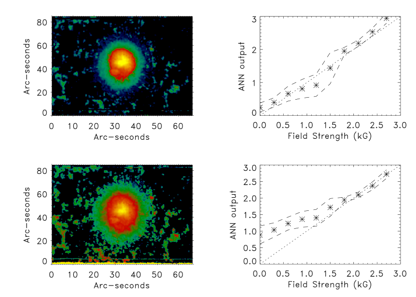
After the time-consuming training process ($\sim$2 days), the ANN was tested with both synthetic and observed ASP data. The results are presented in Fig 5. The performance with synthetic data is very good, as seen in that figure. However, when faced with actual observations, this ANN is unable to provide accurate field estimates below $\sim$1 kG.

The problem with observed profiles is that they exhibit conspicuous features that are not present in the training set. One has moderate to strong asymmetries and other departures from the ideal Milne-Eddington profiles that are unknown to the ANN. This is not so serious in the case of traditional least-squares inversions because those codes find the solution that is closest (in a least-squares sense) to the observation. However, the situation is very different with ANNs. Basically, our network is a multi-dimensional interpolating function, with the training set representing the gridpoints that the interpolating function mimics. When we introduce a point in the ANN that is outside the domain of the training data, the network is forced to perform an extrapolation instead of an interpolation.

There are two different approaches that one might take to overcome this issue. The first one is to take the observed profiles and pre-process them in order to bring them onto the Milne-Eddington hypersurface (see Socas-Navarro 2003 for details). By doing this one is effectively looking for the closest Milne-Eddington profile to the observation. This Milne-Eddington profile is then the one that will be inverted by the ANN. The second approach is to “regularize” the network to make it tolerant to small deviations of the profiles from the ideal shape. Both of these strategies are explored in the next sections.

4 Pre-processing with auto-associative networks

Let us consider first the approach of “projecting” the observed profile vector onto the hypersurface defined by synthetic Milne-Eddington profiles. This is implicitly done by traditional least-squares fitting codes, which find the Milne-Eddington profile that is closest to the observation.

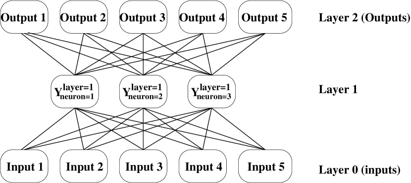
In the context of ANN inversion, the vector projection is not implicit in the method, and this needs to be done explicitly (e.g. as a pre-processing of the input data). In this section I explore a procedure by which an auto-associative neural network (AANN) is used for pre-processing. A previous paper (Socas-Navarro 2004) demonstrated the use of AANNs to decompose and reconstruct spectral Stokes profiles. The reader is referred to that paper for details but a brief explanation of AANNs is given here for completeness. An AANN is simply a neural network that is trained with targets equal to the input data ($o^{t}_{i}=x^{t}_{i}$). (Obviously this requires the same number of neurons in the input and output layers.) An AANN has at least one hidden layer (the “bottleneck” layer) that has fewer neurons than the input/output layers (see Fig 6).

Figure 6: Schematic representation of an auto-associative neural netowrk. Figure reproduced from Socas-Navarro (2004)

For the application presented here we shall depart slightly from the conventional definition of AANNs, but the underlying principle remains the same. One starts by synthesizing a large number of Milne-Eddington profiles that will be used as targets for the AANN. These profiles are then distorted by artificially adding asymmetries, molecular lines with random positions and amplitudes (like those found in the umbra of sunspots) and noise. The quiet Sun intensity profile used for the spatially-unresolved non-magnetic surrounding is randomized so that it is slightly different for each training datapoint. The relative velocity between magnetic and non-magnetic elements is random with an amplitude of 2 km s^-1. Finally, both the perturbed and original profiles undergo basic pre-processing and normalization as explained in §3.

The AANN is trained using the perturbed profiles as inputs and the original Milne-Eddington ones as targets. The bottleneck layer of this network has only 11 neurons, which is also the number of free parameters in the atmospheric model. In principle it should be possible for the AANN to extract a set of 11 parameters from the profiles from which these can then be reconstructed. In practice, however, there may be a significant loss of information due to the limited number of neurons present between the inputs and the bottleneck layer, which in turn limits the complexity of the non-linear transformations that the AANN can do.

Moreover, the problem we are dealing with here is complicated because the inputs have been distorted. This means that the AANN needs to find a suitable set of 11 “features” in the distorted spectra from which it can reconstruct a similar Milne-Eddington profile. Effectively, the AANN is doing the profile projection mentioned earlier, or at least an approximation to it.

Once the AANN is properly trained, we can construct another network that will take the profiles pre-processed by the ANN and do the actual inversion with them. Notice that the “inverting” ANN does not really need to take the full output vector from the AANN. We can simply take the 11-parameter vector in the bottleneck layer. This are the parameters that the AANN has determined contain all the necessary information to reconstruct the Milne-Eddington profiles.

The full data inversion strategy proposed in this section is as follows. We first train an AANN as explained above with distorted profiles as inputs and Milne-Eddington profiles as outputs. Once this network has been trained we shall not make any further use of the layers behind the bottleneck layer. We then construct a second ANN to do the inversion. To generate the training set for this new ANN we must first pre-process all the training profiles with the AANN. Each training profile is propagated through the AANN, but only up to the bottleneck layer. The features in the bottleneck layer are used as inputs to the inverting ANN, whereas the targets are the magnetic field strength properly normalized as in §3.

Figure 7: Results from ANN inversions with the pre-processing approach. Top: Tests with synthetic data. Bottom: Tests with real observations. Left: Maps of the magnetic field stregnth retrieved by the ANN. Right: Comparison plots between the ANN outputs and the magnetic field from the Milne-Eddington inversion. Asterisks: mean value in each bin. Dashed line: Standard deviation of the scatter in each bin. Dotted line: Diagonal of the plot.

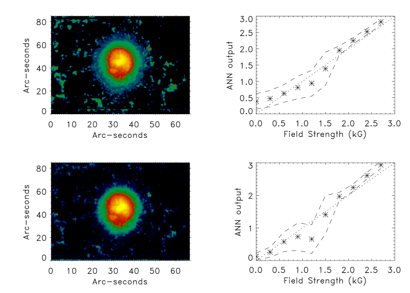
The results of the tests with this complex combination of inputs pre-processing and data inversion are shown in Fig 7. The performance with synthetic profiles has degraded somewhat with respect to the case of the direct approach (Section 3). However, we can see that now the accuracy of inversions with observed and synthetic profiles are very similar. The errors are reasonably small, close to (and sometimes smaller than) 100 G except for the range between 1 kG and 1.5 kG. This region is complicated because it contains most of the quiet Sun fields, which usually have small filling factors. Inverting these profiles is difficult because the polarization signals are typically much weaker (in spite of the fact that the intrinsic field may be strong) and there is rarely any linear polarization at all. The ANN-based inversion tends to underestimate these fields, although the correct solution is still within the 1-$\sigma$ scatter in the plot.

5 Network regularization

The third strategy proposed in this paper is based on the concept of “regularization”, which aims at making the ANN tolerant to small departures from the model. This is usually accomplished by training ANNs with noisy data. In our problem, however, the difficulties reside not only in the noise but more importantly in spurious features such as asymmetries or molecular lines that effectively produce distortions in the profiles.

Regularization may reduce the accuracy of an ANN, especially when working with high-quality data. However, it makes it more robust and improves its generalization ability. One usually needs to find a suitable compromise between these two qualities.

This section explores the applicability of a regularized ANN for the inversion of spectral Stokes data. I have trained a single ANN with input profiles that have been distorted exactly as those for the AANN in §4 and the magnetic fields as targets. The goal is to combine the two steps (pre-processing and inversion) in one. The overall training time is somewhat longer than in previous cases (about 50% longer than the direct approach).

Figure 8: Results from ANN inversions with the regularization approach. Top: Tests with synthetic data. Bottom: Tests with real observations. Left: Maps of the magnetic field stregnth retrieved by the ANN. Right: Comparison plots between the ANN outputs and the magnetic field from the Milne-Eddington inversion. Asterisks: mean value in each bin. Dashed line: Standard deviation of the scatter in each bin. Dotted line: Diagonal of the plot.

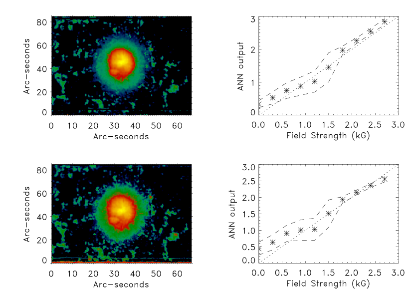
The results of applying this ANN to the test data are shown in Fig 8. As before, the network performance with synthetic data is slightly worse than that of the direct approach. However, we gain an important benefit in that it can invert observations practically with the same accuracy as synthetic data. Compared to the case of §4, this particular ANN performs only a little worse for the weaker fields (below $\sim$1 kG) which are slightly overestimated. These points are found mostly in the outer penumbra (some of them also in the quiet Sun, but they are few). The quiet Sun points between 1 kG and 1.5 kG are better retrieved than in the previous case. There is still a slight underestimation, but the effect is small.

6 Conclusions

This paper shows that ANNs are a viable alternative to least-squares fitting for the routine analysis of large amounts of data. While their accuracy is somewhat lower, the ability to process much larger datasets will probably present advantages for some application. The CPU times required for the ANN inversions presented here are $\sim$10 seconds, compared to $\sim$5 hours for the original Milne-Eddington inversion.

Furthermore, one does not have to be concerned with the algorithm finding secondary minima or not converging. Strictly speaking, the ANN inversion is not an inverse problem. It is rather a case of interpolating a multidimensional function that maps a set of gridpoints from the space of spectra into the space of models.

It is important to emphasize that pattern recognition techniques are not meant to replace traditional least-squares fitting algorithms, but to complement them. For detailed studies of a smaller data subset or individual profiles, or if one needs to consider more realistic model atmospheres (with line-of-sight gradients, Non-LTE effects, etc), it is still necessary to use a least-squares inversion.

References

- Blum & Li (1991) Blum, E. K., & Li, L. K. 1991, Neural Networks, 4, 511
- Carroll & Staude (2001) Carroll, T. A., & Staude, J. 2001, A&A, 378, 316
- del Toro Iniesta (2003) del Toro Iniesta, J. C. 2003, Astronomische Nachrichten, 324, 383
- del Toro Iniesta & López Ariste (2003) del Toro Iniesta, J. C., & López Ariste, A. 2003, A&A, 412, 875
- Elmore et al. (1992) Elmore, D. F., Lites, B. W., Tomczyk, S., Skumanich, A., Dunn, R. B., , Schuenke, J. A., Streander, K. V., Leach, T. W., Chambellan, C. W., Hull, & Lacey, L. B. 1992, in Proc SPIE, Vol. 1746, 22
- Jones (1990) Jones, L. K. 1990, Proceedings of IEEE, 78, 1586
- Keller (1998) Keller, C. U. 1998, Proc. SPIE, 3352, 732
- Landi Degl’Innocenti (1992) Landi Degl’Innocenti, E. 1992, in Solar Observations: Techniques and Interpretation, First Canary Islands Winter School of Astrophysics, ed. F. Sánchez, M. Collados, & M. Vázquez (Cambridge Univ. Press), 71
- Lites (1996) Lites, B. W. 1996, Solar Phys., 163, 223
- Lites et al. (2001) Lites, B. W., Elmore, D. F., & Streander, K. V. 2001, in ASP Conf. Ser., Vol. 236, ”Advanced Solar Polarimetry – Theory, Observation, and Instrumentation”, ed. M. Sigwarth, 33
- Lites et al. (1998) Lites, B. W., Thomas, J. H., Bogdan, T. J., & Cally, P. S. 1998, ApJ, 497, 464
- Rees et al. (2000) Rees, D., López Ariste, A., Thatcher, J., & Semel, M. 2000, A&A, 355, 759
- Rumelhart et al. (1986) Rumelhart, D., Hinton, G., & Williams, R. 1986, in Parallel Distributed Processing: Explorations in the Microstructure of Cognition, ed. D. Rumelhart & J. McClelland (Cambridge, MA: MIT Press), 318
- Sankarasubramanian et al. (2003) Sankarasubramanian, K., Elmore, D. F., Lites, B. W., Sigwarth, M., Rimmele, T. R., Hegwer, S. L., Gregory, S., Streander, K. V., Wilkins, L. M., Richards, K., & Berst, C. 2003, in Polarimetry in Astronomy. Edited by Silvano Fineschi . Proceedings of the SPIE, Volume 4843, pp. 414-424 (2003)., 414–424
- Schmidt et al. (2003) Schmidt, W., Beck, C., Kentischer, T., Elmore, D., & Lites, B. 2003, Astronomische Nachrichten, 324, 300
- Skumanich & López Ariste (2002) Skumanich, A., & López Ariste, A. 2002, ApJ, 570, 379
- Skumanich & Lites (1987) Skumanich, A., & Lites, B. W. 1987, ApJ, 322, 473
- Socas-Navarro (2001) Socas-Navarro, H. 2001, in ASP Conf. Ser. 236: Advanced Solar Polarimetry – Theory, Observation, and Instrumentation, 487
- Socas-Navarro (2003) Socas-Navarro, H. 2003, Neural Networks, 16, 355
- Socas-Navarro (2004) —. 2004, ApJ, submitted
- Socas-Navarro et al. (2001) Socas-Navarro, H., López Ariste, A., & Lites, B. W. 2001, ApJ, 553, 949