A new measurement of the altitude dependence of the atmospheric muon intensity

Abstract

We present a new measurement of atmospheric muons made during an ascent of the High Energy Antimatter Telescope balloon experiment. The muon charge ratio $\mu^{+}/\mu^{-}$ as a function of atmospheric depth in the momentum interval 0.3–0.9 GeV/c is presented. The differential $\mu^{-}$ intensities in the 0.3–50 GeV/c range and for atmospheric depths between 4–960 g/cm² are also presented. We compare these results with other measurements and model predictions. We find that our charge ratio is $\sim$1.1 for all atmospheric depths and is consistent, within errors, with other measurements and the model predictions. We find that our measured $\mu^{-}$ intensities are also consistent with other measurements, and with the model predictions, except at shallow atmospheric depths.

I Introduction

Measurements and theoretical calculations of atmospheric neutrino fluxes have consistently disagreed, and this disagreement was interpreted in terms of neutrino oscillations. However, this interpretation requires an accurate understanding of neutrino fluxes in the atmosphere. Simulations of the absolute fluxes have been conducted (barr:muons ; wentz:muons ; gaisser:muons , and references therein) but suffer from systematic uncertainty in the normalization of the atmospheric neutrino spectrum. These simulations also predict the spectrum of other atmospheric secondaries, specifically muons. Indeed, the production of neutrinos in the atmosphere is closely coupled with that of muons, as they are produced together in pion and kaon decays, and as some muons themselves decay and contribute to the neutrino flux. Therefore, measurements of atmospheric muons by ascending high altitude balloon borne instruments can be used to reduce the neutrino model uncertainties. It should be pointed out that other experimentally accessible quantities can also be used to that end, such as the absolute primary cosmic ray flux impinging on the atmosphere, or other atmospheric secondaries such as gamma rays or secondary nucleons. The atmospheric muon flux is therefore an important element in any comprehensive strategy to improve our understanding of neutrino production in the atmosphere.

An earlier version of the High Energy Antimatter Telescope (HEAT-e^±) instrument had been used to measure air-shower muons during atmospheric ascent coutu:muons . The HEAT instrument is described elsewhere barwick:heat ; beach:heat . In its present configuration, HEAT-pbar is optimized to study antiprotons. It combines a superconducting magnet spectrometer using a drift-tube hodoscope (DTH), a time-of-flight system (TOF), and two stacks of multiwire proportional chambers (dE/dx). We report here a new measurement of the muon charge ratio $\mu^{+}/\mu^{-}$ as a function of atmospheric depth in the momentum interval 0.3–0.9 GeV/c, and differential $\mu^{-}$ intensities in the 0.3–50 GeV/c range and for atmospheric depths between 4–960 g/cm² for a balloon flight from Fort Sumner, NM, USA on June 3, 2000.

II Muon Identification and Backgrounds

The ascent phase of the flight lasted $\sim$3 hours during which more than 1.5 million events were recorded at an average vertical geomagnetic rigidity cutoff of 4.5 GV. The flight occurred under solar maximum conditions ($\Phi$ = 1330 MV). The atmospheric overburden ranged from a high of 960 g/cm² with the instrument on the ground to a low of 4 g/cm² at float altitude.

Muon events were identified using the three main detectors onboard the HEAT-pbar instrument. The methods of muon identification and selection criteria involving the TOF and DTH detectors are described in detail elsewhere coutu:muons . To select muon events using the TOF detector, the incident particle must have $0.85\leq\beta\leq 2.00$, where $\beta=v/c$ is the particle’s velocity in units of the speed of light. Also, for $\mu^{+}$, the particle must have 0.3 GV $<$ R $<$ 0.9 GV and for $\mu^{-}$, R $<$ -0.3 GV, where ${\rm R}=pc/Ze$ is the particle’s magnetic rigidity, or momentum per unit electric charge. Muon events with R $>$ 0.9 GV cannot be selected based on rigidity as a function of $\beta$, due to proton contamination. The range of $\beta$ selected also ensures that the particle was traveling downward through the instrument. To select muon events with the DTH detector, the particle track must have passed through at least 4 of the 8 drift tube planes in the non-bending view, and at least 8 of the 18 planes in the bending view. This is to ensure that there are enough samples along the particle’s track to produce a valid track and rigidity measurement through the DTH. We retain only events with average fit residuals along the track that are better than 6 mm in the x direction, 1.5 mm in the y direction, and 1 mm in the z direction. This rejects only $\sim$0.1% of events, and provides basic track cleanliness criteria. Lastly, the event is required to have a tracking fit goodness parameter $\chi^{2}_{DT}\leq$ 10.0 and $\mid$(Maximum Detectable Rigidity)/R$\mid$ $\geq$ 4, which are used to ensure good track quality.

II.1 The dE/dx Detector

II.1.1 Physical Construction

The dE/dx detector consists of two stacks of 70 segmented multi-wire proportional chambers, one stack above and one below the magnetic hodoscope as shown in Figure 1. The 140 chambers are each $\sim$1 cm thick and filled with a gas mixture of 95% Xenon and 5% Methane (used as a quench gas). Xenon was used since it yields the strongest possible logarithmic rise in the energy loss curve from minimum ionization to relativistic saturation (70%), and hence gives the highest possible velocity resolution.

Figure 1: Schematic view of the HEAT-pbar Instrument. The solid black line labeled “S” is a piece of scintillator and is part of the instrument trigger.

II.1.2 Energy Loss Determination

Each chamber’s anode wires are connected in groups of 4-6 wires. In addition to the ionization energy deposits, there are occasional spurious signals in wire groups away from the particle track. For analysis, only wire groups less than 5 cm (the average width of two adjacent wire groups) from the particle’s track are used in the energy loss determination for each chamber. The signals are corrected for detector response changes during the flight, electronic gain variations, and particle incident angle. Some particle trajectories are within the instrumental acceptance but miss some of the chambers near their edges, so that the mean number of chambers hit in an event is 128 out of 140. We require the particle to have left a signal in at least 103 of 140 chambers to ensure sufficient sampling points for a determination of the average energy loss. The restricted mean average energy loss is determined by eliminating chambers whose signal is not in the lowest 58% of the signals from all chambers hit. The restricted mean average is used to minimize the effects of Landau fluctuations on the final energy loss determination. A typical plot of restricted mean energy loss (dE/dx) versus positive rigidity for ascent data is shown in Figure 2. Included on the plot are the Bethe-Bloch energy loss curves for deuterons, protons, muon/pions, and positrons. Various particle species clearly populate the plot. Note the geomagnetic cutoff effect on the proton data at $\sim$4.5 GV (Fort Sumner, NM, USA).

Figure 2: Distribution of dE/dx as a function of rigidity for ascent data for positive rigidities. Superimposed are the Bethe-Bloch energy loss curves for various particle species.

Figure 3 shows the restricted mean energy loss for events in the rigidity range -0.9 GV $<$ R $<$ -0.3 GV, as an example, which highlights the highly gaussian nature of the restricted mean energy loss. Distributions in other rigidity ranges look similar.

Figure 3: Restricted mean energy loss distributions for ascent data with gaussian fits for -0.9 GV $<$ R $<$ -0.3 GV.

II.1.3 dE/dx Event Selection

For the dE/dx detector, the difference between the restricted mean energy loss for the upper and lower dE/dx stacks must be within approximately two standard deviations from the mean of the difference distribution. This ensures that an event that showers below the top dE/dx stack is rejected. The restricted mean dE/dx signal of the particle must fall between 0 and 65 (inclusive, in arbitrary units) for 0.3 GV $<|$R$|<$ 0.8 GV, between 0 and 70 for 0.8 GV $<|$R$|<$ 4.0 GV, and between 0 and 78 for 4.0 GV $<|$R$|<$ 50.0 GV. See Figure 4 for a plot of restricted mean energy loss versus rigidity.

Figure 4: Restricted mean energy loss as a function of rigidity for ascent data for (top) positive rigidities and (bottom) negative rigidities. The event selections (solid lines) are shown on each plot as well as the Bethe-Bloch energy loss prediction curves (dashed). Note that the apparent higher density of negative muons compared to positive muons is an artifact of the plotting routine used for the figure; there are approximately equal numbers of points shown on each panel.

II.2 Backgrounds to the Differential Muon Intensity

Protons, electrons, and pions are the major background contaminations of the differential muon intensity. The pion intensity, though relatively small with respect to the muon intensity, increases with altitude. From stephens:pions , the pion/muon ratio is $\sim$0.035 at a depth of 3 g/cm². Fortunately, the intensities of other products of atmospheric showers, such as kaons, are small in relation to the muon intensity.

Particle interactions within the HEAT-pbar instrument also produce pions that can contaminate the muon intensity. A GEANT 3.21 Monte Carlo simulation of the instrument with an input proton spectrum falling with an index of $-2.7$ and an input momentum range of 4.5 GV $\leq$ R $\leq$ 50 GV yielded a secondary interaction pion to proton fraction of $1.1\times 10^{-3}$, which decreased to $9.7\times 10^{-5}$ after application of the muon selection criteria. In order to determine what percentage of the muon intensity this represents, and hence the contamination percentage, the proton to muon ratio must be known. As a first order estimate, we used proton and muon information from grieder:CRearth , and determined that the proton-to-muon ratio ranges from $1.6\times 10^{-4}$ at the ground to a maximum of $3.0$ at 13 g/cm². Choosing the highest value for the ratio offers a worst case contamination fraction, since the ratio decreases with depth. Using a ratio of 3.0 yielded an interaction pion intensity that was 0.01% of the proton intensity and 0.03% of the muon intensity at atmospheric depths greater than 13 g/cm². These percentages only decrease further with atmospheric depth, so the interaction pion contamination of the muon intensity is ignored since the error introduced is much less than the statistical error of the measurement. The number of kaons produced in the instrument is even smaller than the pion number, so they are ignored as well.

III Results and Discussion

III.1 Muon Charge Ratio

The number of muons for various atmospheric depths for the rigidity range 0.3 $\leq$ $\mid$R$\mid$ $\leq$ 0.9 GV is shown in Table 1.

Table 1: Muon charge ratio as a function of atmospheric depth (d) for 0.3 $\leq$ $\mid$R$\mid$ $\leq$ 0.9 GV. Errors on the ratios are statistical only.

d	$\overline{d}$	$N_{\mu^{+}}$	$N_{\mu^{-}}$	$N_{\mu^{+}}/N_{\mu^{-}}$
$(g/cm^{2})$	$(g/cm^{2})$
4–7	5.572	228	200	1.14 $\pm$ 0.11
7–13	9.583	428	346	1.237 $\pm$ 0.089
13–32	22.49	910	837	1.087 $\pm$ 0.052
32–67	49.68	1539	1251	1.230 $\pm$ 0.047
67–140	105.2	2460	2099	1.172 $\pm$ 0.035
140–250	190.8	1552	1447	1.073 $\pm$ 0.039
250–350	296.7	658	642	1.025 $\pm$ 0.057
350–840	497.5	949	852	1.114 $\pm$ 0.053
840–960	887.3	688	562	1.224 $\pm$ 0.070

The $\mu^{+}/\mu^{-}$ ratio is shown as a function of atmospheric depth in Figure 5 for a geomagnetic cutoff of $\sim$4.5 GV (Fort Sumner, NM, USA), and in Figure 6 for a very small cutoff at northern latitudes (Lynn Lake, Manitoba, Canada). Shown are the new HEAT-pbar measurements (labeled HEAT 00), as well as two previous HEAT-e^± measurements and other recent measurements (coutu:muons ; boezio:muons ; bellotti:muons ). The various measurements were made at different solar epochs, so that direct comparison is problematic. However, there is good agreement between the various measurements at Fort Sumner, irrespective of the solar modulation conditions, which is to be expected since the primary flux modulation is small above 4.5 GV. There are only two measurements at Lynn Lake, with relatively large uncertainties, and where solar modulation effects are expected to be more important. Both measurements were made under near solar maximum conditions, and are compatible with each other given the large uncertainties. Also shown on Figures 5 and 6 are 3-dimensional calculations of the air shower development with the TARGET algorithm agrawal:target , widely used for neutrino flux calculations. Curves are shown for both solar maximum and minimum conditions, for average primary fluxes (which may not represent the actual spectrum at the time of any individual measurement). The agreement between the calculations and the measurements (especially the HEAT measurements) appears reasonably good, with the caveat that statistical uncertainties at high altitudes for the HEAT 95 measurements are large.

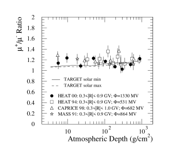
Figure 5: Atmospheric muon charge ratio as a function of atmospheric depth for a geomagnetic cutoff of 4.5 GV (Fort Sumner, NM, USA). Also shown are the ratios for the HEAT 1994 flight as well as other measurements. The curves are calculations with the 3-dimensional TARGET algorithm. Indicated are the solar modulation parameters for each data set.

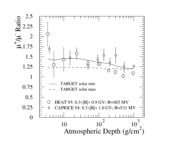
Figure 6: Atmospheric muon charge ratio as a function of atmospheric depth for a geomagnetic cutoff of $\ll$ 1 GV (Lynn Lake, Manitoba, Canada) for two data sets. The curves are calculations with the 3-dimensional TARGET algorithm. Indicated are the solar modulation parameters for each data set.

III.2 $\mu^{-}$ Differential Intensity

Our measurement of the $\mu^{-}$ differential intensities was made using similar corrections as for previous HEAT-e^± flights coutu:muons , with only minor modifications for differing instrument configuration. The results are shown in Figures 7,  8, and 9, and listed in Table 2. The differential intensities as a function of rigidity and atmospheric depth are shown multiplied by $R^{2}$ for better comparison. Also shown are the results of other measurements (boezio:muons ; bellotti:muons ; motoki:muons ). The level of agreement is quite good despite the differing solar epochs and rigidity cutoffs. The curves shown are for calculations with the TARGET algorithm with the same parameters as for Figure 5.

The agreement between the HEAT measurements and model predictions is for the most part excellent, except for the very highest altitudes where the predictions are below the measured intensities. We note that in Fig. 7 there appears to be a tendency for the measurements of the ground $\mu^{-}$ intensities made at a 4.5 GV geomagnetic cutoff to be slightly higher than those at sub-GV cutoff. We do not expect this effect to be real, as energetic muons ($R>1$ GV) at the ground are the end products of parent cosmic rays well above the geomagnetic cutoff at either location. We note that differential intensities are rescaled by $R^{2}$, so that the effect of any small systematic error in the rigidity determination is magnified.

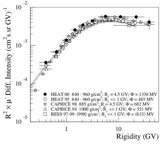
Figure 7: Ground level differential $\mu^{-}$ intensities as a function of rigidity. Also shown are results from various other instruments. The plots have been scaled by a factor of $R^{2}$. The curves are calculations with the 3-dimensional TARGET algorithm for solar minimum (solid) and solar maximum (dashed).

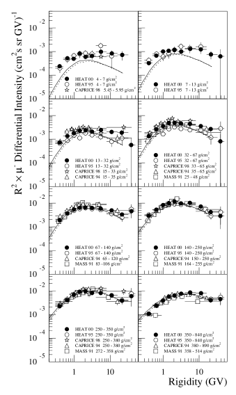
Figure 8: Differential $\mu^{-}$ intensities as a function of rigidity for various atmospheric depth ranges. Also shown are results from various other instruments. (Note: only subsets of measurements by other groups are shown here, where the choice of atmospheric depth bins matches with ours.) The plots have been scaled by a factor of $R^{2}$. The curves are calculations with the 3-dimensional TARGET algorithm for solar minimum (solid) and solar maximum (dashed). See Figures 5 and 6 for each measurement’s solar and geomagnetic conditions.

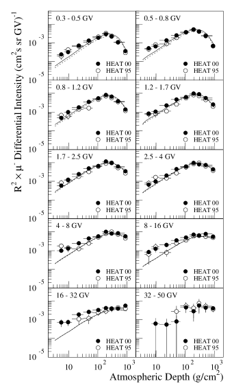
Figure 9: $\mu^{-}$ growth curves for various rigidity intervals. (Note: other groups have used different rigidity bins in their analyses, so that we only report HEAT measurements here.) The plots have been scaled by a factor of $R^{2}$. The curves are calculations with the 3-dimensional TARGET algorithm for solar minimum (solid) and solar maximum (dashed). See Figure 7 for each measurement’s solar and geomagnetic conditions.

Table 2: Atmospheric $\mu^{-}$ intensities [in (cm² s sr GeV/c)^-1] and number of recorded events as a function of rigidity and atmospheric depth.

	4–7 g/cm2	7–13 g/cm2	13–32 g/cm2	32–67 g/cm2	67-140 g/cm2
0.3–0.5	$(1.51\pm 0.26)\times 10^{-3}$	$(2.06\pm 0.31)\times 10^{-3}$	$(4.62\pm 0.61)\times 10^{-3}$	$(8.5\pm 1.1)\times 10^{-3}$	$(1.18\pm 0.15)\times 10^{-2}$
GV	61	108	279	415	672
0.5-0.8	$(1.23\pm 0.18)\times 10^{-3}$	$(1.58\pm 0.21)\times 10^{-3}$	$(3.27\pm 0.41)\times 10^{-3}$	$(6.14\pm 0.74)\times 10^{-3}$	$(8.82\pm 1.09)\times 10^{-3}$
GV	110	186	440	670	1116
0.8–1.2	$(5.21\pm 0.85)\times 10^{-4}$	$(1.02\pm 0.14)\times 10^{-3}$	$(1.84\pm 0.24)\times 10^{-3}$	$(3.61\pm 0.44)\times 10^{-3}$	$(5.58\pm 0.69)\times 10^{-3}$
GV	71	185	380	607	1086
1.2-1.7	$(4.08\pm 0.67)\times 10^{-4}$	$(5.26\pm 0.76)\times 10^{-4}$	$(1.12\pm 0.15)\times 10^{-3}$	$(2.32\pm 0.29)\times 10^{-3}$	$(3.10\pm 0.39)\times 10^{-3}$
GV	71	120	294	498	768
1.7-2.5	$(1.42\pm 0.27)\times 10^{-4}$	$(2.75\pm 0.41)\times 10^{-4}$	$(5.63\pm 0.75)\times 10^{-4}$	$(1.18\pm 0.15)\times 10^{-3}$	$(1.55\pm 0.20)\times 10^{-3}$
GV	41	104	246	415	629
2.5–4.0	$(6.7\pm 1.3)\times 10^{-5}$	$(1.01\pm 0.16)\times 10^{-4}$	$(2.10\pm 0.29)\times 10^{-4}$	$(4.63\pm 0.59)\times 10^{-4}$	$(6.34\pm 0.81)\times 10^{-4}$
GV	37	73	174	311	494
4.0–8.0	$(3.11\pm 0.59)\times 10^{-5}$	$(4.13\pm 0.67)\times 10^{-5}$	$(8.0\pm 1.1)\times 10^{-5}$	$(1.43\pm 0.19)\times 10^{-4}$	$(1.88\pm 0.24)\times 10^{-4}$
GV	43	75	165	239	363
8.0–16.0	$(6.6\pm 1.8)\times 10^{-6}$	$(9.9\pm 2.0)\times 10^{-6}$	$(1.62\pm 0.28)\times 10^{-5}$	$(2.87\pm 0.45)\times 10^{-5}$	$(4.01\pm 0.58)\times 10^{-5}$
GV	17	34	63	90	145
16.0–32.0	$(1.52\pm 0.64)\times 10^{-6}$	$(1.68\pm 0.62)\times 10^{-6}$	$(4.3\pm 1.0)\times 10^{-6}$	$(6.1\pm 1.4)\times 10^{-6}$	$(7.2\pm 1.4)\times 10^{-6}$
GV	6	8	23	25	39
32.0–50.0		$(4.1\pm 4.1)\times 10^{-7}$	$(3.7\pm 3.7)\times 10^{-7}$	$(5.4\pm 5.4)\times 10^{-7}$	$(3.0\pm 1.1)\times 10^{-6}$
GV	0	1	1	1	9

	140-250 g/cm2	250-350 g/cm2	350-840 g/cm2	840-960 g/cm2
0.3–0.5	$(1.88\pm 0.24)\times 10^{-2}$	$(1.40\pm 0.19)\times 10^{-2}$	$(6.69\pm 0.88)\times 10^{-3}$	$(2.28\pm 0.31)\times 10^{-3}$
GV	477	213	247	172
0.5-0.8	$(1.29\pm 0.16)\times 10^{-2}$	$(9.7\pm 1.2)\times 10^{-3}$	$(5.51\pm 0.68)\times 10^{-3}$	$(1.64\pm 0.21)\times 10^{-3}$
GV	730	329	457	283
0.8–1.2	$(8.4\pm 1.1)\times 10^{-3}$	$(6.83\pm 0.86)\times 10^{-3}$	$(3.97\pm 0.49)\times 10^{-3}$	$(1.39\pm 0.18)\times 10^{-3}$
GV	737	359	509	373
1.2-1.7	$(4.84\pm 0.62)\times 10^{-3}$	$(4.37\pm 0.56)\times 10^{-3}$	$(2.74\pm 0.34)\times 10^{-3}$	$(1.22\pm 0.15)\times 10^{-3}$
GV	538	291	448	421
1.7-2.5	$(2.72\pm 0.35)\times 10^{-3}$	$(2.23\pm 0.29)\times 10^{-3}$	$(1.47\pm 0.18)\times 10^{-3}$	$(8.01\pm 0.99)\times 10^{-4}$
GV	501	247	396	457
2.5–4.0	$(1.00\pm 0.13)\times 10^{-3}$	$(8.2\pm 1.1)\times 10^{-4}$	$(7.57\pm 0.95)\times 10^{-4}$	$(4.37\pm 0.54)\times 10^{-4}$
GV	348	171	392	482
4.0–8.0	$(3.34\pm 0.45)\times 10^{-4}$	$(2.67\pm 0.38)\times 10^{-4}$	$(2.69\pm 0.34)\times 10^{-4}$	$(1.77\pm 0.22)\times 10^{-4}$
GV	288	138	349	491
8.0–16.0	$(5.89\pm 0.93)\times 10^{-5}$	$(5.27\pm 0.95)\times 10^{-5}$	$(6.20\pm 0.87)\times 10^{-5}$	$(4.64\pm 0.62)\times 10^{-5}$
GV	95	51	152	230
16.0–32.0	$(9.5\pm 2.4)\times 10^{-6}$	$(8.4\pm 2.6)\times 10^{-6}$	$(9.0\pm 1.9)\times 10^{-6}$	$(1.15\pm 0.18)\times 10^{-5}$
GV	21	12	30	93
32.0–50.0	$(1.9\pm 1.4)\times 10^{-6}$	$(3.9\pm 2.3)\times 10^{-6}$	$(3.0\pm 1.4)\times 10^{-6}$	$(2.66\pm 0.83)\times 10^{-6}$
GV	2	3	5	12

IV Conclusions

We have measured with good statistics the muon charge ratio $\mu^{+}/\mu^{-}$ as a function of atmospheric depth in the momentum interval 0.3–0.9 GeV/c and the differential $\mu^{-}$ intensities in the 0.3–50 GeV/c range and for atmospheric depths between 4–960 g/cm². We have found that our charge ratio is $\sim$1.1 for all atmospheric depths and is consistent, within errors, with other measurements and the model predictions. We have found that our measured $\mu^{-}$ intensities are also largely consistent with other measurements, and with the model predictions, despite varying solar epochs and geomagnetic rigidity cutoffs. This reinforces the conclusion of coutu:muons that model calculations are adequate to the task of predicting neutrino fluxes. The discrepancy between our measurements and the model predictions at shallow atmospheric depths is of little import to our understanding of neutrino fluxes, as the bulk of the neutrinos come from decay processes much deeper in the atmosphere.

- (1) G. Barr et al. Phys. Rev. D (Rapid Comm), 39:3532, 1989.
- (2) J. Wentz et al. Phys. Rev. D, 67(073020), 2003.
- (3) T. K. Gaisser & M. Honda. Ann. Rev. Nucl. Part. Sci., 2002.
- (4) S. Coutu et al. Phys. Rev. D, 62(032001), 2000.
- (5) S. Barwick et al. Nucl. Inst. Meth. A, 400:34, 1997.
- (6) A. S. Beach et al. Phys. Rev. Lett., 87:271101, 2001.
- (7) S. A. Stephens. Proceedings of the 17th International Cosmic Ray Conference (Paris), 4:282, 1981.
- (8) Peter K. F. Grieder. Cosmic Rays at Earth. Elsevier Science B. V., 2001.
- (9) M. Boezio et al. Phys. Rev. D, 67(072003), 2003.
- (10) R. Bellotti et al. Phys. Rev. D, 60(052002), 1999.
- (11) V. Agrawal et al. Phys. Rev. D, 53:1314, 1996.
- (12) M. Motoki et al. Astropart. Phys., 19(113), 2003.