Orbital solutions to the HD 160691 ($\mu$ Arae) Doppler signal

Abstract

We perform a dynamical analysis of the recently updated set of the radial velocity (RV) measurements of the HD 160691 ($\mu$ Arae). The purely kinematic, 2-Keplerian model of the measurements leads to the best-fit solution in which the eccentricity of the outer planet is about 0.7 and its semi-major axis is about 4 AU. The parameters of the inner planet are well determined. The eccentricity is about 0.3 and the semi-major axis is about 1.65 AU. In such circumstances, the best 2-Keplerian model leads to a catastrophically unstable configuration, which is self disrupting in less than 20,000 yr. In order to derive dynamically stable configurations which are simultaneously consistent with the RV data, we use the so called GAMP (Genetic Algorithm with MEGNO Penalty) which incorporates the genetic fitting algorithms and a verification of the stability by the fast indicator of the dynamics (MEGNO). Using this method, we derive meaningful limits on the parameters of the outer planet which also provide a stable behavior of the system. It appears, that the best-fit solutions are located in a shallow valley of ${(\chi^{2}_{\nu})^{1/2}}$, in the $(a_{{\mbox{\scriptsize c}}},e_{{\mbox{\scriptsize c}}})$-plane, extending over 2 AU (for the formal $1\sigma$ confidence interval of the best fit). We find two equally good best-fit solutions leading to the qualitatively different orbital configurations. One of them corresponds to the center of the 5:1 mean motion resonance (MMR) and the second one describes a configuration between the 6:1 and 17:2 MMRs. Generally, the HD 160691 system can be found in the zone confined to other low-order MMRs of the type $p$:1 with $p>5$. Our results support the classification of the $\mu$ Ara as a hierarchical planetary system, dynamically similar to other known multi-planet systems around HD 12661 and HD 169830. The results of the GAMP analysis on the extended data set are fully consistent with our previous conclusions concerning a much shorter observational window. It constitutes a valuable confirmation that the applied method is well suited for the analysis of the RV data series which only partially cover the longest orbital period.

1. Introduction

Precise measurements of the radial velocity (RV) of two stars, HD 160691 ($\mu$ Ara ) and HD 154857, from the Anglo-Australian survey for extrasolar planetary systems have been recently published by McCarthy et al. (2004). Our particular attention is devoted to the HD 160691 system. Butler et al. (2001) reported a planet with a 2 yr orbital period about the $\mu$ Ara . This discovery was confirmed by Jones et al. (2002b) and the observational window extended to 4 yr revealed an additional linear trend in the RV signal, interpreted as the signature of a more distant planet. The data presented in the new paper by the Anglo-Australian Planet Search team cover about 6 yr. This extended observational window allows to confirm the existence of the second Jovian planet in the system. Very recently, Santos et al. (2004) discovered a small, $14~{}$-Earth masses object in a circular orbit, at the distance of only 0.09 AU from the $\mu$ Ara star and confirmed the findings of (McCarthy et al., 2004). The Anglo-Australian team determined the Keplerian elements of the Jovian companions: the orbital periods of 645 d, 3000 d and the eccentricities of 0.2, 0.57, respectively (McCarthy et al., 2004). According to these authors, the current data set covers about 70% of the longer period.

The detection of multiple, Jovian-like planets in stages from shorter to longer orbital periods are obviously expected from the Doppler surveys and (McCarthy et al., 2004) announce another possible multiple system around HD 154857. It is interesting to follow the subsequent estimations of the orbital parameters of such system, derived on the basis of an increasing number of observations. In the preprint by Jones et al. (2002a), the preliminary orbital solution for $\mu$ Ara suggested a proximity of the two putative planets to the 2:1 mean motion resonance (MMR). Such configuration would be the third occurrence of this particular low-order resonance among only about 15 multi-planet systems known at that time. However, the formal 2-Kepler solution found in the preprint appeared to be very unstable. In the published paper, Jones et al. (2002b) excluded the possibility of the 2:1 MMR due to an increased orbital period of the outer planet (by about 300 d). Our independent analysis of the same RV data set (Goździewski et al., 2003) has revealed that in the specific case of $\mu$ Ara , when one has only a part of the orbital RV signal of the additional planetary companion, the application of 2-Kepler model of RV signal certainly leads to artifacts. The formally best-fit configurations are self-disrupting on a short time-scale! The newest set of measurements leads to the 2-Kepler solution with the outer planets’ period increased to $\simeq 3000$ d (McCarthy et al., 2004). This 2-Keplerian fit still describes a configuration which disintegrates after only $20,000$ yr. It can be easily checked by direct integration of the 3-body problem. In fact even a simple analysis shows that this best fit is located in the proximity of the planetary collision zone. The exact collision curve can be determined through $a_{{\mbox{\scriptsize b}}}(1+e_{{\mbox{\scriptsize b}}})=a_{{\mbox{\scriptsize c}}}(1-e_{{\mbox{\scriptsize c}}})$. This means that the large eccentricity of the companion c would be possible only if an orbital dynamical mechanism protecting the planets from an encounter existed. Another possibility is that the real orbital elements are in fact different from those determined by McCarthy et al. (2004).

Clearly, one needs a method of dynamical analysis of the orbital fits which will reproduce an observed RV signal and simultaneously fulfill stability criteria. In our method, we not only account for the mutual interactions between the planets (Laughlin & Chambers, 2001) but also eliminate the orbital fits corresponding to strongly chaotic orbits, regardless of their goodness of fit expressed by ${(\chi^{2}_{\nu})^{1/2}}$. We treat the dynamical behavior in terms of the chaotic and regular (or weakly-chaotic) states as an observable, at the same level of importance as the RV measurements are. Details of the algorithm which will be called from hereafter the Genetic Algorithm with MEGNO Penalty (GAMP) are presented in (Goździewski et al., 2003). This method seems to be particularly useful for systems undergoing strong mutual interactions such as the $\mu$ Ara system. According to the quoted preliminary estimates of the semi-major axes of the companions and their eccentricities, the likely configurations are related to the zone of strong low-order mean motion resonances like 5:2, 4:1, 5:1, 6:1, 7:1. The widths of these resonances rapidly increase with the growing eccentricity of the outer companion, finally leading to their overlapping and a creation of a zone of global instability (see section 4 in this work). In this instance, the MMRs-originating chaotic diffusion leads to violent, macroscopic changes in the physical state of the system (Froeschlé & Lega, 1999). In a planetary system, it means close encounters between the planets and/or the parent star, collisions or ejection of a body from the system. Following this reasoning, to find configurations which are stable over long periods of time, it is essential to eliminate the strongly chaotic solutions. These solutions originate in the unstable MMRs and lead to a discontinuity of the searched parameter space, in the sense of the dynamical stability. The sophisticated structure of the phase space can be understood in terms of the KAM theorem. Obviously, both the kinematic models of the Doppler signal as well as the gradient-like methods of the RV data fitting which require the ${(\chi^{2}_{\nu})^{1/2}}$ to be a continuous function of its variables, are not well suited to this case. On the contrary, the discontinuous structure of the orbital parameter space justifies the application of non-gradient fitting and Monte-Carlo based techniques.

Taking into account these very basic considerations, we analyzed the RV data published by Jones et al. (2002b). We found that the quasi-linear trend present in the reflex motion of HD 160691 permitted a continuum of equally good solutions in the $(a_{{\mbox{\scriptsize c}}},e_{{\mbox{\scriptsize c}}})$-plane. Moreover, using the GAMP algorithm and assuming that $a_{{\mbox{\scriptsize c}}}<5$ AU, it was possible to reduce the space of stable fits, permitted by the RV data, to a number of solutions confined to the zone of low-order mean motion resonances (MMRs) like 3:1, 7:2, 4:1, 9:2, 5:1, 11:2, 6:1. Moreover, the short observational window did not permit a distinction between them. At present, having the access to the updated observations, we have an occasion to verify these early predictions and to test the reliability of the fits obtained with GAMP. Many stars accompanied by Jovian planets reveal linear trends in the Doppler signal indicating the presence of additional companions (e.g., Butler et al., 2003). Hence, we have a chance to test if our method is helpful in obtaining preliminary and realistic estimates of their orbital parameters.

2. The numerical setup

As the basic tool for searching for the best fit solutions to the RV data, we use the genetic algorithm scheme (GA) implemented by Charbonneau (1995) in his publicly available code named PIKAIA. The synthetic reflex motion of the star is described by the 2-Keplerian RV model (as in Goździewski et al., 2003) and the self-consistent Newtonian, $N$-body model (Laughlin & Chambers, 2001) incorporating the MEGNO indicator penalty (Goździewski et al., 2003). It is known that the genetic scheme is not efficient for finding very accurate best-fit solutions but provides good starting fits for much faster and more precise gradient methods, like the Levenberg-Marquardt (LM) algorithm (Stepinski et al., 2000). Nevertheless, the GA makes it possible, in principle, to find the global minimum of ${(\chi^{2}_{\nu})^{1/2}}$ while the gradient methods are basically local. In our experiments, the GA fits were finally refined by a yet another very accurate non-gradient minimization scheme by Melder and Mead (Press et al., 1992), widely known as the simplex method. The fractional convergence tolerance to be achieved in the simplex code has been set in the range $10^{-6}$–$10^{-9}$. Typically, the lower accuracy has been forced by time consuming GAMP tests. The application of the simplex refinement in the CPU expensive GAMP code is essential because it reduces the CPU usage dramatically (by a factor of ten, at least).

For the stability analysis, we use two numerical tools which are helpful in resolving the regular (quasi-periodic) and irregular (chaotic) character of a tested configuration. The already mentioned MEGNO algorithm (Cincotta & Simó, 2000; Cincotta et al., 2003; Giordano & Cincotta, 2004) is already used in a few our papers. In this work (also to avoid a routine approach in our stability studies), we apply an alternative method derived on the basis of the Fast Fourier Transform (FFT). This spectral method (SM) was developed by Michtchenko & Ferraz-Mello (2001). Its idea is very simple: in the quasi-periodic system, the spectral signal, (here $f(t)=a(t)\exp(\mbox{i}\lambda(t)$ where $a(t)$ and $\lambda(t)$ are the heliocentric canonical elements (Laskar & Robutel, 1995), the semi-major axis and mean longitude, respectively), has only a small number of leading frequencies while in the chaotic system the spectrum of these frequencies becomes very complicated. By counting the number of the frequencies (the spectral number, $SN$) in the FFT spectrum of the signal that have amplitudes over a given noise level (typically, we use a threshold of about a few percent of the largest amplitude), one can distinguish between a regular and chaotic motion. It appears that these two fast indicators are similarly well sensitive to the chaotic diffusion generated by the MMRs in the systems with Jupiter-like planets and the required integration time is relatively very short, typically, about $10^{4}$ periods of the outermost planet. The spectral method seems to have many advantages. Its simplicity is appealing. Under certain conditions, the SM is even more efficient than MEGNO because one avoids integrating complex variational equations. It provides a straightforward identification of the MMRs. To summarize the differences between the two methods, one could say that the SM detects the chaotic diffusion as an ”analogue” device, while the MEGNO (Lyapunov exponent type indicator) is more of a ”digital” tool. Details of the comparison of these two complementary methods will be described elsewhere.

3. Searching for the Newtonian best fits

First, we performed the analysis of the 2-Keplerian fits to the RV data of the HD 160691 system similarly to (Goździewski et al., 2003). The best fit solution has ${(\chi^{2}_{\nu})^{1/2}}=1.644$ and the rms of $4.147$ m/s (see Table 1). This fit is catastrophically unstable. It is not surprising because $e_{{\mbox{\scriptsize c}}}\simeq 0.72$ by far exceeds eccentricities corresponding to the collision curve for the two planets. Our 2-Keplerian fit has significantly larger $e_{{\mbox{\scriptsize c}}}$ and the orbital period of the outer planet than found by the discovery team. At present, $P_{{\mbox{\scriptsize c}}}\simeq 3360$ d is also longer than from the previous 2-Keplerian estimate (Jones et al., 2002b; Goździewski et al., 2003). This conclusion and our experiments (not only from this work) seem to follow an empirical rule: if the measurements cover only a fragment of the longest orbital period, widening the observational window leads to an even longer period. Obviously, the current set of RV data still does not permit to identify a stable solution, when assuming the purely kinematic 2-Keplerian model of the RV data. The synthetic RV curve of the best 2-Keplerian fit in Fig. 1 is barely different from the curve corresponding to the synthetic curve derived from the $N$-body model (more details will be given further). Yet, they describe completely different configurations. Obviously, their ${(\chi^{2}_{\nu})^{1/2}}$ and rms must be almost the same. This example clearly shows that the smallest ${(\chi^{2}_{\nu})^{1/2}}$ or rms cannot be the decisive factor for the choice of the proper description of the observed planetary configuration.

In the next experiments, we used only the full $N$-body model of the reflex motion of the parent star. The first question is how (if at all) the self-consistent fits (for the moment—without the instability penalty) change the character of the best fit solutions. Such fits have been initialized by the GA and refined by the simplex. The results are illustrated in Fig. 2. It shows the projections of the best fits to which the simplex converged in every individual run (expressed by osculating heliocentric elements) on the planes of the relevant orbital parameters. Hundreds of independent runs of the fitting code have been preformed. The osculating elements are given at the moment of the first observation. The best fit solution is given in Table 1 as the NL1 fit. Its rms is about 4.15 m/s and ${(\chi^{2}_{\nu})^{1/2}}\simeq 1.643$, thus almost the same as for the 2-Keplerian model. Yet, the derived minimal mass of the outer planet is much smaller than in the 2-Keplerian solution.

The collected fits make it possible to obtain a general view of the orbital configurations of the system permissible by the $N$-body model. It appears that the elements of the inner planet are already well fixed. This is not the case for the outer companion. Its eccentricity, in the range of $1\sigma$ confidence interval of the best fit solution NL1, can vary over 0.1-0.8 and the semi-major axis spreads over 2-3 AU. Also the mass of the outer planet cannot be precisely estimated. Surprisingly, the angular elements of both companions are relatively well bounded. Assuming a coplanar configuration, this result makes it possible to reduce the space of barely determined parameters to three dimensions: $(M_{{\mbox{\scriptsize c}}},a_{{\mbox{\scriptsize c}}},e_{{\mbox{\scriptsize c}}})$. This is quite comfortable for the studies of the system dynamics because it can be limited to a representative $(a_{{\mbox{\scriptsize c}}},e_{{\mbox{\scriptsize c}}})$-plane parameterized by the mass of the outer companion. The assumption of coplanarity may be justified by the recent results (Santos et al., 2004). As we already mentioned, these authors discovered a small, Neptune-like planet around the HD 160691 . They also measured the projection of the rotational velocity, $v\sin i$, of HD 160691 and found it close to the theoretical, maximal value. Let us suppose that the orbital plane of the smallest planet is almost perpendicular to the rotational axis of HD 160691 . This means that the orbit is almost ”edge-on”. In the presence of a possibly highly inclined Jovian planet, the orbit of the smaller companion would be influenced by the Kozai resonance. For a large relative inclination, this mechanism forces a large eccentricity of the inner, smaller body and finally can destabilize its motion. Because the eccentricity of the inner planet is very small (Santos et al., 2004), the two most inner orbits should not be significantly inclined. Assuming that the planetary system emerged from a coplanar proto-planetary disk, the whole system is likely close to the coplanar configuration. Still, the recent results by Thommes & Lissauer (2003) and Adams & Laughlin (2003) indicate that a large fraction of planetary systems which interact gravitationally can be in fact significantly non-coplanar. Unfortunately, the currently available data do not permit to investigate such a possibility.

As we have already noticed, the NL1 solution is formally as good as the fit obtained with the 2-Kepler model. Unfortunately, there is also a similar problem with the stability of the relevant configuration. The evolution of the orbital elements (Fig. 3) clearly shows that the motion is strongly chaotic and, in fact, corresponds to collisional orbits. In the specific integration, the Lyapunov time is only 233 yr. It will be shown later that this fit corresponds to the border of 5:1 MMR (Fig. 10).

In order to estimate the formal errors of the best fit NL1, we followed Goździewski & Maciejewski (2003). The actual error of the determination of the RV consists of two parts: the measurement error and the contribution from the variability of the star itself. For chromospherically quiet G and K dwarfs the stallar jitter is about the level of the measurements errors. In this paper we adopted $\sigma_{{\mbox{\scriptsize jitter}}}\simeq 3$ m/s, following the estimates of the stellar variability of G dwarfs by McCarthy et al. (2004) (see their Fig. 1). These estimates are based on 6 yr monitoring of a few representative G-type stars similar to $\mu$ Ara . To estimate the error of the best fit NL1, we added to every original measurement a random Gaussian noise with the zero mean value and the mean dispersion $\sigma\simeq 4$ m/s and the Gaussian noise of the stellar jitter with $\sigma_{{\mbox{\scriptsize jitter}}}\simeq 3$ m/s. Next, the best fit was recalculated with the simplex algorithm using the synthetic data set. This procedure was repeated 5000 times. After finding the mean values of the best fit parameters, we calculated their dispersions. These dispersions are used as the estimates of the mean errors of the osculating elements and shown in parentheses in Table 1. These estimates confirm our earlier findings indicating that the planetary phases can be relatively well fixed while the mostly unconstrained elements are the mass, the semi-major axis and the eccentricity of the outer planet.

Further, to see whether the formal RV errors increased by a contribution from the stellar jitter influence the overall distribution of the best fit elements, we repeated the GA search using the original data points and their mean errors changed to $\sigma\rightarrow\sqrt{\sigma^{2}+\sigma_{{\mbox{\scriptsize jitter}}}^{2}}$. The parameters of the best fit found in this search are given in Table 1 as the NL2 solution and the distribution of the best fit elements is shown in Fig. 4 and Fig. 5. Obviously, the larger mean errors do not lead to a significant modification of the overall distribution of the best fits. Let us note that the projections shown in Fig. 2,4 and 5 serve as an alternative, realistic estimation of the fit errors. The errors obtained in this way are even larger than the previously derived.

The experiments utilizing the $N$-body model of the RV measurements confirm that the existence of the second planetary companion. Nevertheless, all the best-fit initial conditions still lead to self-disrupting configurations and, additionally, are not well constrained. Recalling the discussion in the introduction and the results of dynamical analysis in Goździewski et al. (2003), we already have a rough picture of the phase space in the relevant zone of $(a_{{\mbox{\scriptsize c}}},e_{{\mbox{\scriptsize c}}})$. This zone is confined to strong, unstable low-order MMRs. Due to the preferably large initial $e_{{\mbox{\scriptsize c}}}$, the chances of finding stable configurations by a straightforward Keplerian or Newtonian fit to the RV data are poor.

Thus, to find the best-fit orbital solution in a zone of stability, we have made extensive calculations by applying the GAMP. The code has been restarted hundreds of times. The control parameters of the code have been changed and adjusted to give an additional degree of randomness in the GA search. The results are illustrated in Fig. 6. As in the previous cases, this figure shows a projection of the found best-fit solutions onto different planes of osculating elements. Only those fits are shown which have ${(\chi^{2}_{\nu})^{1/2}}<1.668$. This limit corresponds to the formal $1\sigma$ confidence interval of the best fit solution (GM1, see Table 1) having ${(\chi^{2}_{\nu})^{1/2}}=1.64701$ and rms 1.147 m/s. As we can expect, the stable solutions have $e_{{\mbox{\scriptsize c}}}<0.5$. This strongly confirms our prediction from Goździewski et al. (2003).

The reader may notice that the ${(\chi^{2}_{\nu})^{1/2}}$ for GM1 (Table 1) is given with an unusually high precision of 5 decimal places. This is due to another solution (GM2, see Table 1) having almost the same ${(\chi^{2}_{\nu})^{1/2}}$ while its $a_{{\mbox{\scriptsize c}}}$ is shifted by 0.4 AU. The orbital behavior of the corresponding configurations (see Fig. 7 and Fig. 8) clearly shows that they belong to qualitatively different dynamical regimes. The GM1 fit corresponds to a very stable, regular behavior which is confirmed by the MEGNO rapidly converging over 1 Myr. Surprisingly, the GM2 fit describes a system whose stability is marginal. This system is trapped into the 5:1 MMR. This is illustrated in panel Fig. 7c showing one of the critical arguments of the resonance, $\sigma_{{\mbox{\scriptsize 5:1}}}=5\lambda_{{\mbox{\scriptsize c}}}-\lambda_{{\mbox{\scriptsize b}}}-\varpi_{{\mbox{\scriptsize c}}}-3\varpi_{{\mbox{\scriptsize c}}}$.

4. Dynamics and stability analysis

In principle, the best-fit solutions found by the GAMP search should be dynamically stable. The chaos in the GM2 solution can be explained by a relatively short integration time used in the algorithm (about 1000 $P_{{\mbox{\scriptsize c}}}$ at 5 AU) which does not allow to eliminate mildly chaotic configurations. We assume here that the chaos manifestating through a linear growth of MEGNO after a relatively long time (much longer than adopted in the GAMP) is regarded as a week one. This can be considered as a desired property of the method rather than its drawback. In fact, it can hardly be expected that multi-planet extrasolar systems found so far should be strictly quasi-periodic and regular, in terms of the Lyapunov exponent. Nevertheless, due to the fast convergence of the MEGNO and its great sensitivity to the chaotic evolution, the short integration times make it possible to eliminate the strongly chaotic configurations which very likely would lead to significant changes of the orbital elements. To verify the long-term stability of the best fit solutions found in this way, we should always analyze the structure of the phase space in their vicinity. Such analysis (using numerical or analytical tools) helps us to explore the dynamical environment of the nominal configuration, estimate whether the fits are robust to the errors and the found configurations do not change qualitatively under small adjustments of the initial conditions.

First, we have examinated the GM1 fit by computing the stability map in the $(a_{{\mbox{\scriptsize c}}},e_{{\mbox{\scriptsize c}}}$)-plane using the SM code. The relevant orbital parameters were varied and other elements were fixed at the values quoted in Table 1. The results of this test are illustrated in Fig. 9. The integration time for this map is $\simeq 10^{5}$ yr ($\simeq 10^{4}$ orbital periods at 5 AU). The best fit solution is marked by a big circle. The planetary collision line for fixed initial $a_{{\mbox{\scriptsize b}}},e_{{\mbox{\scriptsize b}}}$ is depicted as a smooth curve. The dynamics over this line or in its proximity is very chaotic and the planets’ eccentricities grow rapidly to $1$, indicating collisions or ejections from the system. As we could expect, the stability map reveals an amazingly complex and beautiful structure of MMRs. These MMRs can be easily identified. It appears that the GM1 fit is close to the border of the 11:2 and 17:2 MMRs. In the previous paper on the HD 160691 system, we already suggested that this system may be very similar do the HD 12661 planetary system. It appears that, according to the current best-fit solutions, the dynamical environment of HD 160691 may be a close analogue of this system. Let us recall that in Goździewski & Maciejewski (2003) we found that the HD 12661 may be located close to the 6:1 MMR while the orbital fits of Butler et al. (2003) are related to the proximity of 11:2 MMR (Goździewski, 2003). Due to the mentioned tendency that the estimated orbital period of the outermost body increases with a longer observational time span, the proximity of the HD 160691 system to 6:1 MMR may also be quite possible.

A similar stability test has been performed for the GM2 solution (Fig. 10). The upper panel is for the SM stability map in the ($a_{{\mbox{\scriptsize c}}},e_{{\mbox{\scriptsize c}}})$-plane. The middle panel is for the maximum eccentricity of the planet c attained during the integration period. In both plots the best fit is marked with a big circle. For comparison, in the stability map (Fig. 10, upper panel), the solution corresponding to NL1 fit is marked with a smaller circle. Note that due to very similar orbital elements in the NL1 and GM2 fits, depicting both of them at the same stability map is reasonable. Now it is clear why the NL1 fit leads to a chaotic configuration. According to the identification of MMRs in this map, the GM2 fit is inside the libration island of the 5:1 MMR, while the NL1 fit lies in a close vicinity or within the separatrix of this resonance.

In the $\max e_{{\mbox{\scriptsize c}}}$-map (Fig. 10, the middle panel), we also marked (small circles) all fits gathered in the GAMP search within $1\sigma$ confidence interval of the best fit solutions GM1, GM2. Such illustration of the best fit solutions is justified because, as we already mentioned, $(a_{{\mbox{\scriptsize c}}},e_{{\mbox{\scriptsize c}}})$-plane is representative for the dynamical state of the system. The distribution of the best fits in this plane makes it possible to derive some interesting conclusions. In spite of the fact that the points representing the fits are spread over $a_{{\mbox{\scriptsize c}}}\in[4,6)$ AU, the tendency of a decreasing $e_{{\mbox{\scriptsize c}}}$ with larger values of $a_{{\mbox{\scriptsize c}}}$ is clear. Extrapolating this trend, the outer planet should have a small initial eccentricity for large $a_{{\mbox{\scriptsize c}}}\simeq 6$–$7$ AU. The acceptable fit values within the $1\sigma$ error of $e_{{\mbox{\scriptsize c}}}$ can be varied over 0–0.4. Similarly to the previously analyzed LN1 and LN2 fits, the distribution of the osculating elements in the ($a_{{\mbox{\scriptsize c}}},e_{{\mbox{\scriptsize c}}}$)-plane gives us an insight into realistic error estimates of these orbital elements.

Obviously, all the relevant fits ”avoid” the neighborhood of the collision zone. Close to and over the collision line, $\max e_{{\mbox{\scriptsize c}}}$ grows to 1 which means that the system should be disrupted. The comparison of the stability maps for the GM1 and GM2 shows that the width of the MMRs significantly depends on the particular orbital parameters. Nevertheless, their positions do not change much. Let us recall, that the stability maps in Fig. 9 and 10 correspond to $a_{{\mbox{\scriptsize c}}}$ altered by about 0.5 AU and $e_{{\mbox{\scriptsize c}}}$ by $\simeq 0.1$.

The last panel shown in Fig. 10 refers to the maximum of the argument $\theta=\varpi_{{\mbox{\scriptsize c}}}-\varpi_{{\mbox{\scriptsize b}}}$ attained during the integration time. Librations of $\theta$ correspond to the so called secular apsidal resonance (SAR) when the planetary apsides remain aligned or anti-aligned. The behavior of $\theta$ is important for the discussion of the dynamics of 2-planet configurations in the absence of strong MMRs. In this instance, the motion of the planetary system may be averaged over the mean longitudes. The secular behavior of the averaged system can be described in terms of the secular octupole theory of hierarchical planetary systems by Lee & Peale (2003b) and the recent more general secular theory of 2-planet systems by Michtchenko & Malhotra (2004). According to the results of these authors, the generic 2-planet coplanar system which is far from low-order MMRs and collision zones exhibits a long-term stable behavior. This behavior can be characterized by the time evolution of $\theta$. This angle can librate about $0^{\circ}$ or $180^{\circ}$, circulate, or librate about $0^{\circ}$ in the large-eccentricity regime corresponding to the true secular resonance (for details see Michtchenko & Malhotra, 2004). When the eccentricities are moderate, the two first possibilities (modes) are alternative for the secular evolution of the planetary system. Under some conditions (Lee & Peale, 2003b), the SAR regime appears with a probability close to 1.

The octupole secular theory by Lee & Peale (2003b) is well suited for the HD 160691 system in the range of $a_{{\mbox{\scriptsize c}}}>4$ AU and under the assumption that a given initial condition (IC) is distant from low-order MMRs. In this case, the best-fit solutions are characterized by a relatively small ratio $\alpha=a_{{\mbox{\scriptsize b}}}/a_{{\mbox{\scriptsize c}}}\simeq 0.3$, as for hierarchical configurations. The bottom panel in Fig. 10 illustrates the extent of the SAR in the range of $a_{{\mbox{\scriptsize c}}}\in[4,6]$ AU. Besides the centers of the MMRs, the SAR with the anti-aligned apsides appears over an extended range of $a_{{\mbox{\scriptsize c}}}$ and for relatively small $e_{{\mbox{\scriptsize c}}}$. Let us recall that this map has been derived numerically, simultaneously with calculating the SM stability map. It is very well reproduced by means of the octupole theory, see the map in the left panel in Fig. 11, which is obtained by the numerical integration of the averaged equations of motion (Lee & Peale, 2003b, a). Another SAR map of the secular system, computed in the eccentricities plane, is shown in the right panel of Fig. 11. In both of these maps, the best fit GM1 is found in the extended zone of circulations of $\theta$. Figure 12 illustrates the evolution of $\theta(e_{{\mbox{\scriptsize b}}})$ and $\theta(e_{{\mbox{\scriptsize c}}})$ for the IC defined by GM1. These plots have been derived by the numerical integration of the full $N$-body equations of motion. The phase plots are computed for the constant values of the semi-major axes and the total angular momentum, $J$. Let us recall that the averaged system is governed by 1 degree of freedom Hamiltonian in which $\theta$ and the eccentricity of one planet are the relevant canonical variables. To construct the phase plots, we fixed the initial $\theta$ either at $0^{\circ}$ or $180^{\circ}$ and $e_{{\mbox{\scriptsize b}}}$ was varied appropriately while the other initial eccentricity, $e_{{\mbox{\scriptsize c}}}$, was derived from the $J$ integral. The fact that the phase curves are not ideally smooth can be explained by the proximity to the two MMRs, 11:2 and 17:3. This confirms that the GM1 fit corresponds to the configuration with $\theta$ confined to the extended zone of circulation. The large amplitudes of eccentricities shown in Fig. 8 can be also explained by the phase plots.

The secular features of the GM1 configuration remind us of another hierarchical system about HD 169830. The dynamical environments of their secular configurations are very similar. For instance, compare the discussed figures with the corresponding ones from Goździewski & Konacki (2004) (their Fig. 14 and Fig. 15). The appearance of the SAR in extrasolar systems with well separated giant companions is not an extraordinary feature as sometimes claimed. In the light of the mentioned secular theories, in the regime of moderate eccentricities, the secular systems should be found in one of two distinct regimes of stable motion characterized by the circulation of librations of the critical argument $\theta$. Nevertheless, one should be aware that the secular theories give us only an approximate description of the long-term behavior. In the proximity to the strong MMRs, the stability should be investigated by an application of theories suitable for every individual resonance or long-term direct integrations.

5. Conclusions

The new RV data of the HD 160691 system published by the Anglo-Australian Planet Search team McCarthy et al. (2004) enable us to refine the orbital best-fit solutions. The preliminary observations published in Jones et al. (2002b) suggested the presence of the second companion inducing a linear trend in the RV signal. In the light of the currently available data, it is very likely that the semi-major axis of the outer planet cannot be smaller than about $4$ AU. This makes the system relatively separated. Curiously, the kinematic 2-Keplerian model of the RV signal constantly produces artifacts e.g. the apparent proximity to the 2:1 MMR or large eccentricities of the outer companion. These configurations lead to collisions between the planets in a very short time. In this work, we applied the ”dynamical” fitting by forcing a requirement that a real system should not be disrupted over a short time-span (thousands of years). Our analysis with the proposed GAMP algorithm reveals that the current data set still does not well constrain the semi-major axis of the outer companion. But the requirement of dynamical stability puts strong limits on the initial eccentricity of the outermost planet. The current set of observations is equally well modeled by a continuum of statistically equivalent best-fit solution which are distributed over $a_{{\mbox{\scriptsize c}}}\in[4,6)$ AU and $e_{{\mbox{\scriptsize c}}}$ about $[0-0.4]$, along a flat valley of ${(\chi^{2}_{\nu})^{1/2}}$ in the $(a_{{\mbox{\scriptsize c}}},e_{{\mbox{\scriptsize c}}})$-plane of osculating orbital parameters. Surprisingly, the initial longitudes of the coplanar configurations seem to be already well fixed.

The dynamical analysis of the best-fit solutions reveals that the currently determined parameters of the outer planet are confined to the zone of low order MMRs with the inner planet, like 5:1, 11:2, 6:1, 13:2, 7:1. The distribution of the best solutions, within the formal $1\sigma$ confidence interval of the best fit, reveals a clear correlation between initial values of $a_{{\mbox{\scriptsize c}}}$ and $e_{{\mbox{\scriptsize c}}}$—the larger semi-major axis of the outer planet, the smaller its initial eccentricity. According to the empirically observed law, the increase of the observational window results in the increase of the determined orbital periods. This would mean that in the current best fit $a_{{\mbox{\scriptsize c}}}\simeq 4.79$ AU is still smaller than the real value. It is difficult to predict the real $a_{{\mbox{\scriptsize c}}}$ but very likely it is in the range $[5,6]$ AU.

During the final preparation of this paper, we have learned about a discovery of a Neptunian-mass body in the HD 160691 system, close to the parent star (Santos et al., 2004). The semi-major axis of this small planet is about $0.09$ AU. Obviously, it is interesting to verify whether the presence of this body can affect the best-fit solutions and the dynamical behavior of the whole planetary system. The RV measurements published by the Anglo-Australian Planet Search team have the mean errors comparable to the RV semi-amplitude variations imposed by the new planet (4 m/s). For the moment, the newest observations, as reported in the discovery paper, span a very short period of time (at present, about 80 d). Unfortunately, these measurements are not available. They would be very helpful in improving our fits because they cover the end-part of the longer period and should constrain the parameters of the outer companion. We tried to refine our fits using the data from a scanned figure published by the Swiss team on their WWW page. The full data set, produced by a combination of the Anglo-Australian measurements and these synthetic RV points, has been firstly modeled using the $N$-body signal. We used velocity offsets different for the two observatories. Still, we encountered similar problems as in the case of the Anglo-Australian data itself. The best $N$-body fits for the 3-planet system converge to $a_{{\mbox{\scriptsize c}}}\simeq 3.8$ AU and $e_{{\mbox{\scriptsize c}}}>0.6$. According to the stability analysis, such fits locate the Jovian planets in a strongly chaotic zone. For the 3-planet best-fit solutions, we have ${(\chi^{2}_{\nu})^{1/2}}\simeq 1.56$ and the rms of $\simeq 3.6$ m/s. Assuming that the innermost planet does not disturb the motion of the Jovian companions too much and applying the GAMP for these two planets only (otherwise, the CPU time requirement is very significant), we derived solutions qualitatively similar to the GM1 and GM2 fits (although the rms of these solutions exceeds $4.7$ m/s). They tend to have a large $e_{{\mbox{\scriptsize c}}}\simeq 0.5$. Simultaneously, through the requirement of stability, the GAMP places the best fits about $a_{{\mbox{\scriptsize c}}}\simeq 5.5~{}AU$. Thus, in spite of a better time coverage, the curious inconsistency between the pure $N$-body and the GAMP-derived solutions is still evident. These results can only be preliminary. A reliable modeling of the RV data is a difficult task without having access to the actual measurements.

Although the elements of the innermost planet seem to be determined, due to the barely determined parameters of the outer planet, we think that the dynamical studies concerning the whole system do not make at present a great sense. As we have shown, the two Jovian planets can be coupled by a strong, low-order MMRs or can be well separated and relatively far from MMRs. These situations create completely different dynamical environments for the whole planetary system.

In terms of the overall dynamical behavior, the $\mu$ Ara system appears to be similar to the HD 12661 and to the HD 169830. The Jovian planets in these systems are well separated. The variation of eccentricities spans a similar, relatively extended range from 0 to 0.5-0.6. Their semi-major axes ratio corresponds to a proximity of low-order MMRs, like 6:1 or 11:2 (for the HD 12661) or 7:1, 8:1 (similar to the HD 169830). Whether a real link exists between these systems is not clear at the moment. We still have to wait for new observations which eventually make it possible to derive significantly accurate determination of their parameters.

Using the GAMP algorithm we performed a very preliminary analysis of the RV data of the HD 154857 system. Similarity to the HD 160691 , these data reveal the presence of one Jovian planet and a linear trend, indicating the presence of the second, more distant body. Our $N$-body fits make it possible to approximate the elements of this planet: its mass is about 0.5 M${}_{{\mbox{\scriptsize J}}}$, semi-major axis about $4$ AU and large eccentricity $\simeq 0.78$. Of course, these elements are barely constrained. Nevertheless, the parameters of the inner planet are quite well fixed and we can already compute the stability map of this system. It is shown in Fig. 13. The relevant zone is filled up by strong MMRs, similarly to the HD 160691 system. By the same reasoning, as applied to the HD 160691 system, the eccentricity of the outer planet should be strongly limited by the requirement of dynamical stability.

Our work advocates a dynamical analysis of the RV data. Even if the observational window covers only partially the longest orbital period, we are able to derive a lot of characteristics of the discussed system, avoiding falsifying the orbital elements by the purely kinematic approach. In fact, the analysis presented in this paper shows that the application of the GAMP-like algorithm is essential for finding reliable solutions which well reproduce the RV data and simultaneously lead to orbitally stable configurations of the planetary companions.

6. Acknowledgments

This work is supported by the Polish Committee for Scientific Research, Grant No. 2P03D 001 22. K.G. is also supported by the UMK grant 428-A. M.K. is also supported by NASA through grant NNG04GM62G.

Table 1 Initial conditions of the HD 160691 system. The first column is for the best 2-Kepler fit expressed in Jacobi elements, according to the model in Goździewski et al. (2003). Fit marked by NL1 is derived by the self-consistent $N$-body fitting and expressed by osculating heliocentric Keplerian elements at the moment of first observation (JD=2,450,915.2911). The NL2 solution is derived by the same approach, when the measurement errors are scaled by the stellar jitter ($\simeq 3$ m/s). Fits denoted by GM1 and GM2 are formally the best fits obtained in the GAMP search. The osculating heliocentric Keplerian elements are given at the date of first observation. The mass of the parent star is equal to $1.08~{}\mbox{M}_{\sun}$.

	2K		NL1		NL2		GM1		GM2
Parameter	b	c	b	c	b	c	b	c	b	c
$\mbox{m}_{2}\sin i$ [M${}_{{\mbox{\scriptsize J}}}$]	1.675	7.675	1.674 (0.068)	2.707 (0.898)	1.683	5.689	1.670	2.981	1.677	2.398
a [AU]	1.499	4.551	1.497 (0.007)	4.325 (0.560)	1.499	4.683	1.497	4.788	1.498	4.364
P [d]	644.7	3368.7
e	0.202	0.719	0.201 (0.029)	0.470 (0.215)	0.203	0.585	0.204	0.340	0.201	0.411
$\omega$ [deg]	115.14	348.53	114.83 (6.37)	341.14 (16.23)	115.15	347.03	116.89	343.15	116.42	342.70
$T_{{\mbox{\scriptsize p}}}$ [JD-2,450,000]	2196.8	3681.4
$M$ [deg]			4.68 (4.54)	49.79 (26.13)	3.67	66.50	1.45	65.2	2.75	46.42
${(\chi^{2}_{\nu})^{1/2}}$	1.64378		1.64464		1.12871		1.64701		1.64707
RMS [m/s]	4.15		4.15		4.12		4.17		4.15
$V_{0}$ [m/s]	-37.2		-22.08 (6.12)		-33.37		-22.08		-16.49

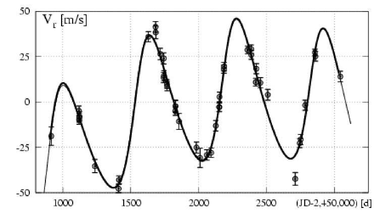
Figure 1.— Synthetic radial velocity curves for the HD 160691 system. The thin line is for the best 2-Keplerian solution (2K, see Table 1). The thick line is for a stable, $N$-body fit GM1 (see the text for explanation). Open circles are for the RV measurements published in (McCarthy et al., 2004).

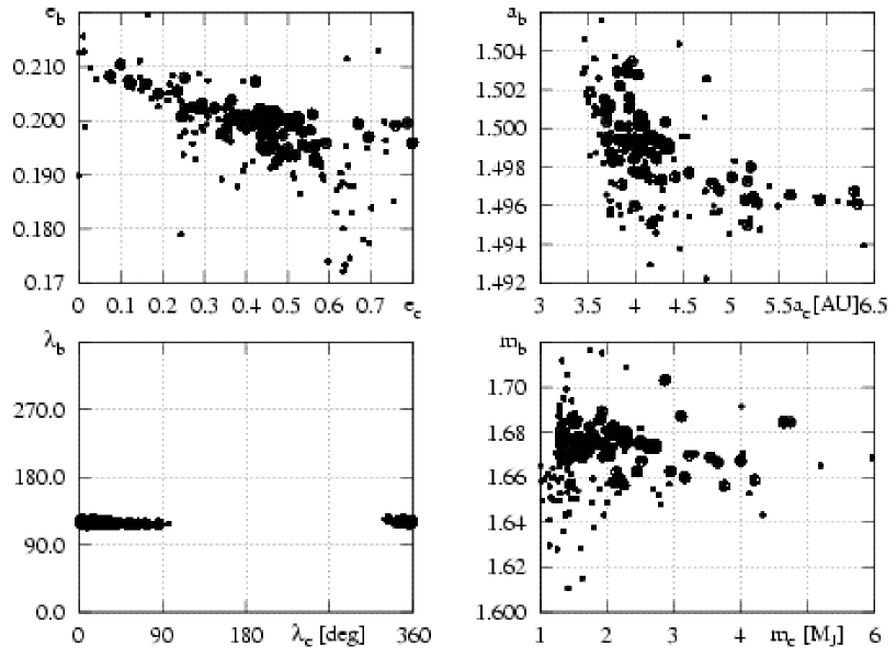
Figure 2.— The best fits obtained by the Newtonian model for the RV data published in McCarthy et al. (2004). Small filled circles are for solutions with ${(\chi^{2}_{\nu})^{1/2}}$ within the formal $3\sigma$ confidence interval of the NL1 fit (see Table 1, ${(\chi^{2}_{\nu})^{1/2}}<1.75$). Bigger, open circles are for ${(\chi^{2}_{\nu})^{1/2}}<1.667$ corresponding to $1\sigma$ confidence interval of the best fit NL1. Largest filled circles are for the fits of ${(\chi^{2}_{\nu})^{1/2}}<1.646$, marginally larger, by about 1%, from the ${(\chi^{2}_{\nu})^{1/2}}\simeq 1.644$ of the best fit solution NL1.

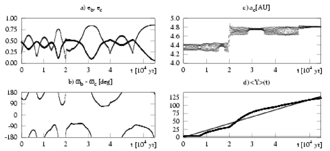
Figure 3.— Orbital behavior in the best self-consistent, Newtonian fit NL1. Panel a) is for the eccentricities. Panel b) is for the argument of the SAR. Panel c) is for the semi-major axis of the outer companion. Panel d) is for the MEGNO, $\langle Y\rangle$. The thin line illustrates the linear fit $\langle Y\rangle(t)=(\lambda_{{\mbox{\scriptsize max}}}/2)t+d$. The derived Lyapunov time, $T_{L}=1/\lambda_{{\mbox{\scriptsize max}}}$, is about 233 yr.

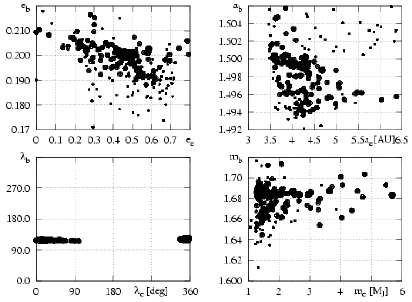
Figure 4.— The best fits obtained by the Newtonian model of the RV data and their errors scaled by the stellar jitter with the mean dispersion about 3 m/s (see the text for explanation). Small filled circles are for solutions with ${(\chi^{2}_{\nu})^{1/2}}<1.277$, within the formal $3\sigma$ confidence interval of the NL2 fit (see Table 1). Bigger, open circles are for ${(\chi^{2}_{\nu})^{1/2}}<1.16$ corresponding to $1\sigma$. Largest filled circles are for the fits of ${(\chi^{2}_{\nu})^{1/2}}<1.130$, marginally larger, by about 1%, from the ${(\chi^{2}_{\nu})^{1/2}}\simeq 1.129$ of NL2.

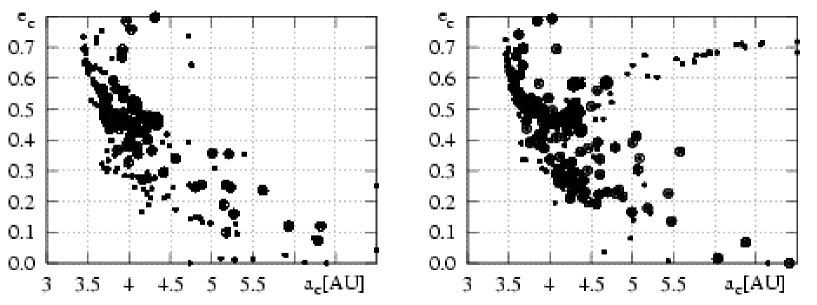
Figure 5.— A comparison of the distribution of the best fits obtained by the $N$-body fitting in the $(a_{{\mbox{\scriptsize c}}},e_{{\mbox{\scriptsize c}}})$-plane. The left panel is for the original data set, the right panel is for the case when the measurements error are scaled by the stellar jitter (see the text for explanation). The meaning of symbols is the same as in Fig. 2 and 4, respectively.

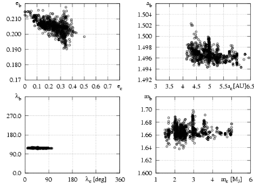
Figure 6.— The best fits obtained by the GAMP. Open circles are for ${(\chi^{2}_{\nu})^{1/2}}<1.668$, i.e., within formal $1\sigma$ confidence interval of the best fit solution having ${(\chi^{2}_{\nu})^{1/2}}=1.647$.

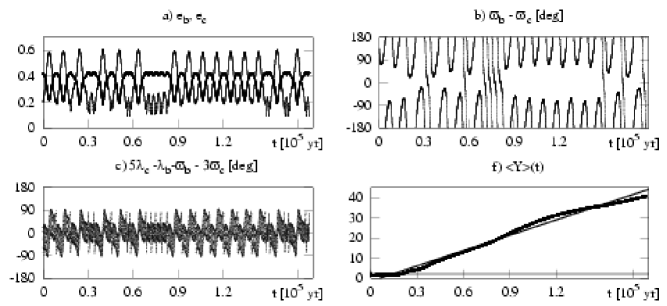
Figure 7.— Orbital behavior in the GM2 fit. Panel a) is for the eccentricities. Panel b) is for the argument of the SAR. Panel c) is for the critical argument of the 5:1 MMR. Panel d) is for the MEGNO, $\langle Y\rangle$. The thin line illustrates the linear fit $\langle Y\rangle(t)=(\lambda_{{\mbox{\scriptsize max}}}/2)t+d$. The derived Lyapunov time, $T_{L}=1/\lambda_{{\mbox{\scriptsize max}}}$, is about 35,000 yr.

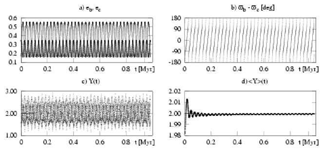
Figure 8.— Orbital behavior in the GM1 fit. Panel a) is for the eccentricities. Panel b) is for the argument of the SAR. Panel c) is for the the temporal MEGNO, $Y(t)$. Panel d) is for the MEGNO, $\langle Y\rangle$.

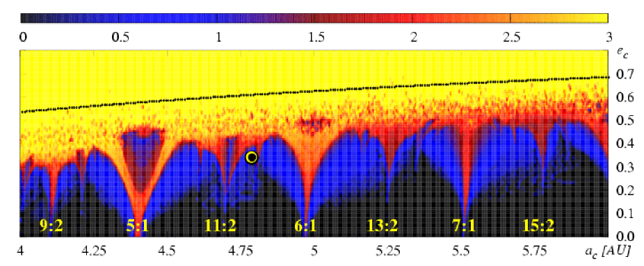
Figure 9.— The stability map in the $(a_{{\mbox{\scriptsize c}}},e_{{\mbox{\scriptsize c}}})$-plane, in terms of the spectral number, $\log SN$, (see the text for an explanation) for the best fit solution GM1 (see Table 1). Color code is for $\log SN$: black means quasi-periodic, regular configurations, and yellow strongly chaotic systems. Labels are for the identification of the low-order MMRs. A big circle marks the parameters of the GM1 fit.

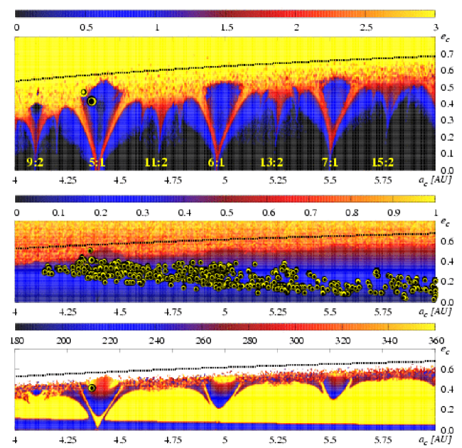
Figure 10.— The upper plot is for the stability map in the $(a_{{\mbox{\scriptsize c}}},e_{{\mbox{\scriptsize c}}})$-plane, in terms of the spectral number, $\log SN$, (see the text for an explanation) for the best fit solution GM2 (see Table 1). Color code is for $\log SN$: black means quasi-periodic, regular configurations and yellow strongly chaotic systems. A big circle marks the parameters of the GM2 fit. For comparison, the elements of NL1 fit are depicted as a smaller circle. The middle plot is for maximum eccentricity of the outer planet attained during the integration period (about $10^{5}$ yr). Circles in this plot mark parameters of the fits obtained in the GAMP search within $1\sigma$ confidence interval of the GM1 fit. The lower plot is for the maximum of $\theta$. The resolution of the maps is is $600\times 100$ data points.

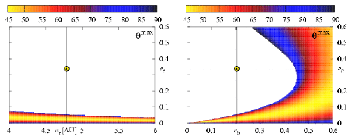
Figure 11.— The semi-amplitude of the critical argument of SAR, $\theta$, about the libration center $180^{\circ}$, derived by the application of the secular octupole theory by Lee & Peale (2003b, a). The nominal parameters of the GM1 fit are marked by circles and intersecting lines. Compare with the lower plot in Fig. 10.

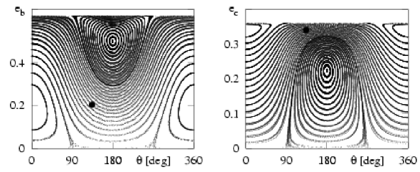
Figure 12.— Phase diagram of the GM1 fit obtained by numerical integration of the full, $N$-body model for constant values of the integrals of the total angular momentum and total energy. The nominal configuration is marked by a filled circle in both panels. See the text for explanation.

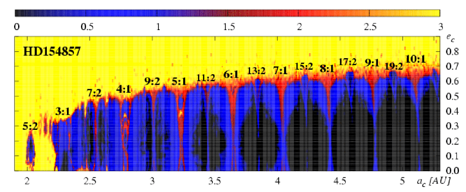
Figure 13.— The stability map in the $(a_{{\mbox{\scriptsize c}}},e_{{\mbox{\scriptsize c}}})$-plane, in terms of the spectral number, $SN$, for the HD 154857 planetary system. Color code is for $SN$: black means quasi-periodic, regular configurations and yellow (light gray) strongly chaotic systems. Labels are for the identification of the low-order MMRs. Resolution of the plot is $640\times 100$ data points.

References

- Adams & Laughlin (2003) Adams, F. C. & Laughlin, G. 2003, Icarus, 163, 290
- Butler et al. (2003) Butler, R. P., Marcy, G. W., Vogt, S. S., Fischer, D. A., Henry, G. W., Laughlin, G., & Wright, J. T. 2003, ApJ, 582, 455
- Butler et al. (2001) Butler, R. P., Tinney, C. G., Marcy, G. W., Jones, H. R. A., Penny, A. J., & Apps, K. 2001, ApJ, 555, 410
- Charbonneau (1995) Charbonneau, P. 1995, ApJS, 101, 309
- Cincotta et al. (2003) Cincotta, P. M., Giordano, C. M., & Simó, C. 2003, Physica D, 182, 151
- Cincotta & Simó (2000) Cincotta, P. M. & Simó, C. 2000, A&AS, 147, 205
- Froeschlé & Lega (1999) Froeschlé, C. & Lega, E. 1999, in NATO ASIC Proc. 522: The Dynamics of Small Bodies in the Solar System, A Major Key to Solar System Studies, 463–+
- Giordano & Cincotta (2004) Giordano, C. M. & Cincotta, P. M. 2004, A&A, 423, 745
- Goździewski & Konacki (2004) Goździewski, K. & Konacki, M. 2004, ApJ, 610, 1093
- Goździewski et al. (2003) Goździewski, K., Konacki, M., & Maciejewski, A. J. 2003, ApJ, 594
- Goździewski & Maciejewski (2003) Goździewski, K. & Maciejewski, A. J. 2003, ApJ, 586, L153
- Goździewski (2003) Goździewski, K. 2003, A&A, 398, 1151
- Jones et al. (2002a) Jones, H., Butler, P., Marcy, G., Tinney, C., Penny, A., C., M., & B., C. 2002a, MNRAS, astro-ph/0206216
- Jones et al. (2002b) Jones, H. R. A., Paul Butler, R., Marcy, G. W., Tinney, C. G., Penny, A. J., McCarthy, C., & Carter, B. D. 2002b, MNRAS, 337, 1170
- Laskar & Robutel (1995) Laskar, J. & Robutel, P. 1995, Celestial Mechanics and Dynamical Astronomy, 62, 193
- Laughlin & Chambers (2001) Laughlin, G. & Chambers, J. E. 2001, ApJ, 551, L109
- Lee & Peale (2003a) Lee, M. H. & Peale, S. J. 2003a, ApJ, 597, 644
- Lee & Peale (2003b) —. 2003b, ApJ, 592, 1201
- McCarthy et al. (2004) McCarthy, C. et al. 2004, ApJ
- Michtchenko & Ferraz-Mello (2001) Michtchenko, T. & Ferraz-Mello, S. 2001, ApJ, 122, 474
- Michtchenko & Malhotra (2004) Michtchenko, T. A. & Malhotra, R. 2004, Icarus, 168, 237
- Press et al. (1992) Press, W. H., Teukolsky, S. A., Vetterling, W. T., & Flannery, B. P. 1992, Numerical Recipes in C. The Art of Scientific Computing (Cambridge Univ. Press)
- Santos et al. (2004) Santos, N. C. et al. 2004, A&A, 426, L19
- Stepinski et al. (2000) Stepinski, T. F., Malhotra, R., & Black, D. C. 2000, ApJ, 545, 1044
- Thommes & Lissauer (2003) Thommes, E. W. & Lissauer, J. J. 2003, ApJ, 597, 566