Curvature Perturbations from Broken Symmetries

Abstract

We present a new general mechanism to generate curvature perturbations after the end of the slow-roll phase of inflation. Our model is based on the simple assumption that the potential driving inflation is characterized by an underlying global symmetry which is slightly broken.

I Introduction

One of the most successful predictions of the inflationary theory, the current paradigm for understanding the evolution of the early universe guth81 , is the redshifting of quantum fluctuations of the field driving inflation – the inflaton – beyond the Hubble radius, leading to an imprint on the background scalar (density) and tensor (gravitational waves) metric perturbations lrreview ; muk81 ; hawking82 ; starobinsky82 ; guth82 ; bardeen83 ; Hu:2004xd ; Mukhanov:1990me ; Durrer:2004fx ; Langlois:2004de ; Brandenberger:2003vk that subsequently seeds structure formation.

For simplicity, most inflation models assume that there is only one scalar field involved in the dynamics of inflation. This is also the case when the mechanism of converting the energy driving inflation into radiation is considered. In this work we point out a qualitatively new effect that might arise if one relaxes the assumption of a single dynamical field. In a multi-field scenario in which the inflationary potential is characterized by a broken symmetry, the quantum fluctuations generated during the inflationary stage represent fluctuations in the initial conditions for the dynamics of the inflaton in the subsequent stage, thus implying that the background dynamics after the slow-roll phase has ended will differ in different regions of the universe. Since the background fields are coupled to the other fields into which they decay, the fluctuations generated during the slow-roll phase will affect the subsequent decay process.

The present work, assuming that the inflaton decay into other fields through the non-perturbative process of preheating Kofman:1997yn ; Felder:1998vq , is then aimed to understand whether isocurvature inflaton fluctuations, generated during the slow-roll stage, can lead to perturbations of the background metric through variations of the preheating efficiency. While the generation of curvature perturbations during the stages following the slow-roll phase has already been considered in some works Dvali:2003em ; Dvali:2003ar ; Matarrese:2003tk ; Lyth:2001nq ; Liddle:1999hq ; Wands:2000dp ; Malik:2002jb ; Gupta:2003jc , the present work is the first one to show that in a multi-field scenario a global broken symmetry of the potential is sufficient to yield curvature perturbations. Curvature perturbations produced through this mechanism can even represent the main source of perturbations to the background metric if the inflationary potential is such that the mass required to produce quantum fluctuations along the field trajectory is large, so that the latter result exponentially suppressed.

The structure of the present work is the following. In Sec. II we obtain a general formula for the curvature perturbations generated from an inhomogeneous preheating efficiency related to the quantum fluctuations produced during inflation. Sec. III presents an application of the general result obtained in Sec. II to the case of a broken $U(1)$ symmetry. The conclusions are contained in Sec. IV.

II General Results

One of the main objectives in any particular preheating model is the calculation of the comoving number density of particles produced during the process, usually denoted by $n_{\chi}$. In general, $n_{\chi}$ is a functional of the evolution and of the couplings of the preheat field $\chi$ to the dynamically evolving field(s): $n_{\chi}=F[\vec{\phi}(t)]$, where $\vec{\phi}=\phi_{1},\ \phi_{2},\ \cdots,\ \phi_{n}$ denotes the background inflaton fields that couple to $\chi$. Choosing a specific preheating model is then equivalent to specifying the functional $F$ that relates $\vec{\phi}(t)$ to $n_{\chi}$.

In general, the dynamics of the background fields and of the scale factor is given by the solution of the system of coupled differential equations

$$\ddot{\phi}_{i}+3H\dot{\phi}_{i}+\frac{\partial V}{\partial\phi_{i}}=0,\quad i=1,...,n,$$ (1a)

$$H^{2}=\left(\frac{\dot{a}}{a}\right)^{2}=\frac{8\pi}{3M_{p}^{2}}\left[\sum_{i}\frac{\dot{\phi}_{i}^{2}}{2}+V(\vec{\phi})\right],$$ (1b)

once the particular landscape of the potential $V(\vec{\phi})$ and a set of initial conditions $\{\vec{\phi}(t_{0}),\dot{\vec{\phi}}(t_{0})\}$ are specified.

The main subject of the present work is to analyze how quantum fluctuations generated during the slow-roll stage of inflation may affect the efficiency of the subsequent preheating process. As inflation proceeds, quantum fluctuations will in fact cause the value of the background inflaton field to fluctuate in space about a mean value $\vec{\phi}_{0}(t)$:

$$\vec{\phi}(t,x)=\vec{\phi}_{0}(t)+\delta\vec{\phi}(t,x).$$ (2)

Denoting by $t_{0}$ the epoch when inflation has ended but preheating has not yet commenced, it is possible to note that Eq. (2) above shows that at each point in space the initial conditions $\vec{\phi}(t_{0},x)$ that will determine the subsequent background field dynamics through Eqs. (1a,1b) are affected by the quantum fluctuations produced during inflation. Since the preheating efficiency is related to the dynamics of the background, it is then possible to conclude that quantum fluctuations produced during inflation may lead to fluctuations in the preheating efficiency through different background dynamics.

Broken Symmetry. It is then necessary to point out that the mere presence of quantum fluctuations in the initial conditions for the dynamics of the background during the preheating stage are not sufficient to yield different background evolutions leading to fluctuations of the preheating efficiency. If in fact the background potential $V(\vec{\phi})$ is perfectly symmetric – that is $V(\vec{\phi})=V(|\vec{\phi}|)$—then the fluctuations in the initial conditions will only lead to background evolutions that are time translations of each other: in this case a simple rotation of the coordinate system in field space would again yield the well know case of a single scalar field. If the inflationary potential is characterized by a broken symmetry, on the other hand, then fluctuations in the initial conditions will lead to background trajectories that are not just time translations of one another. Two such background trajectories are shown in Fig. 1 for the case of a two-dimensional field space. Notice that the minimum distance to the origin in the trajectories are different. If the efficiency of the preheating process depends on the minimum distance obtained in the trajectory, then the preheating history will differ.

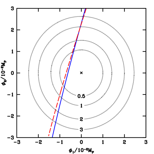
Figure 1: Two background trajectories arising from fluctuations in the initial conditions in the case in which the background field space is two dimensional. Also shown are the equipotential contours (units of $10^{-16}M_{p}^{4}$). The potential used in this figure is the one given in Eq. (16) and further analyzed in Sec. III, which is characterized by a global $U(1)$ broken symmetry. In this case, and for illustration purposes only, the symmetry breaking parameter has been arbitrarily set to $x=0.15$.

Initial Conditions. It is important to distinguish here between the “initial conditions” for the background dynamics specified at the beginning of the slow-roll phase and those specified at time $t_{0}$, that is once the slow-roll phase has terminated and the preheating phase has not yet commenced. Since the present work deals with the particle production during preheating, the term “initial conditions”—and their fluctuations—refers here to the initial conditions for the preheating phase, that is to $\vec{\phi}(t_{0},x)$.

Considering the presence of the friction term $3H\dot{\phi}_{i}$ in Eqs. (1a), it also seems reasonable to assume that the background dynamics during the preheating stage is mostly affected by the position that the background occupies in field space at the beginning of such a phase. Since the comoving number density of particles produced during preheating is a functional of the background trajectory, it is then possible to conclude that

$$n_{\chi}=n_{\chi}[\vec{\phi}(t_{0}),...].$$ (3)

Let’s then turn to the preheating process and to the generation of curvature perturbations. As a first approximation, let’s assume that preheating is complete and that the products of preheating are therefore the only particles populating the universe when the preheating stage has ended. Neglecting the possible contributions stemming from non-adiabatic pressure perturbations present during the preheating stage, an estimate for the curvature perturbation $\zeta$ can be obtained considering the number density perturbation,

$$\zeta\equiv\psi-H\frac{\delta\rho_{\chi}}{\dot{\rho}_{\chi}}\approx\alpha\frac{\delta n_{\chi}}{n_{\chi}},$$ (4)

where the spatially flat gauge has been assumed and the proportionality constant $\alpha$ depends on the redshifting of the particle produced. The above expression then allows to obtain an estimate of the curvature perturbations produced during the preheating stage induced by the fluctuations in the initial conditions $\delta\vec{\phi}(t_{0})$ present at the beginning of such a stage because of the preceding inflationary stage. To proceed further it is then necessary to note that the coordinate system chosen to express the potential is not necessarily the one suited to analyze the perturbations arising during inflation, since in this coordinate system adiabatic and isocurvature perturbations are not decoupled. Adiabatic perturbations are most commonly thought to be the ones dominating the energy density during the inflationary stage, while the isocurvature ones are usually considered not to affect the energy density. Recalling the work of by Gordon et al. Gordon:2000hv , it is also possible to note that given the inflationary trajectory $\vec{\phi}(t)$, adiabatic perturbations correspond to perturbations along the direction tangent to the trajectory $\dot{\vec{\phi}}(t)$, while isocurvature perturbations correspond to perturbations in the hyperplane orthogonal to $\dot{\vec{\phi}}(t)$. This point can be intuitively understood once Eq. (1a) is considered: since the motion of the background is driven by the gradient of the potential, it is reasonable to expect that the trajectory will be tangent to the gradient. This in turn means that perturbations perpendicular to the trajectory will necessarily be isocurvature perturbations since they lie on equipotential hypersurfaces (thus perturbing the field values but not the energy density). Perturbations along the direction of the trajectory, on the other hand, being orthogonal to equipotential hypersurfaces, will necessarily affect the value of the energy density and therefore correspond to adiabatic perturbations. To decouple adiabatic and isocurvature perturbation it is then necessary to rotate the field space coordinate system so that one of the unit vectors lies along the tangent to the trajectory. Let’s first of all define the unit vector $\hat{u}_{\parallel}$ which points in the direction of field space parallel to the (tangent to the) trajectory by

$$\hat{u}_{\parallel}=\frac{\dot{\vec{\phi}}(t_{0})}{|\dot{\vec{\phi}}(t_{0})|},$$ (5)

which allows to determine the component of the perturbation parallel to the trajectory simply by $\delta\phi_{\parallel}=\delta{\vec{\phi}}(t_{0})\cdot\hat{u}_{\parallel}$. Using the latter, it is then possible to define the unit vector $\hat{u}_{\perp}$ which is orthogonal to the (tangent to the) trajectory by

$$\hat{u}_{\perp}=\frac{\delta\vec{\phi}(t_{0})-\delta\phi_{\parallel}\hat{u}_{\parallel}}{|\delta\vec{\phi}(t_{0})-\delta\phi_{\parallel}\hat{u}_{\parallel}|},$$ (6)

which then leads to the component of the perturbation orthogonal to the trajectory $\delta\phi_{\perp}=\delta{\vec{\phi}}(t_{0})\cdot\hat{u}_{\perp}$. A new coordinate system in field space has then been defined, and the perturbation $\delta\vec{\phi}(t_{0},x)$ has been decomposed accordingly:

$$\delta\vec{\phi}(t_{0},x)=\delta\phi_{\parallel}\hat{u}_{\parallel}+\delta\phi_{\perp}\hat{u}_{\perp}.$$ (7)

In this new coordinate system $\delta\phi_{\parallel}$ represents an adiabatic perturbation while $\delta\phi_{\perp}$ represents an entropy perturbation. It is now quite intuitive to note that if the potential is characterized by a broken symmetry, then while adiabatic perturbations of the initial conditions $\delta\phi_{\parallel}$ will lead to background trajectories that are differing just by a time translation, entropy perturbations will lead to trajectories that substantially differ from each other and that will therefore produce variations of the preheating efficiency.

With this redefinition of the coordinate system of field space it is then possible to estimate the variation of the comoving density of particles produced during preheating due to fluctuations in the initial conditions generated during inflation. Note in fact that

$$\frac{\delta n_{\chi}}{n_{\chi}}=\frac{\partial\ln(n_{\chi})}{\partial\phi_{\parallel}}\delta\phi_{\parallel}+\frac{\partial\ln(n_{\chi})}{\partial\phi_{\perp}}\delta\phi_{\perp}=\nabla\ln(n_{\chi})\cdot\delta\vec{\phi}(t_{0},x),$$ (8)

but since perturbations of the initial conditions parallel to the field velocity will simply lead to background evolutions that are time translations of each other it is possible to conclude that $\partial\ln(n_{\chi})/\partial\phi_{\parallel}=0$ and that the mechanism under analysis is thus able to convert entropy perturbations into adiabatic ones. Also, it is possible to envision models in which the inflationary dynamics is such that the adiabatic perturbations $\delta\phi_{\parallel}$ are exponentially suppressed. Combining Eqs. (4) and (8) it is therefore possible to conclude that an estimate of the curvature perturbations produced by the inhomogeneous preheating efficiency connected to fluctuations in the background field dynamics originated during the inflationary phase is given by

$$\zeta\approx\alpha\frac{\partial\ln(n_{\chi})}{\partial\phi_{\perp}}\delta\phi_{\perp},$$ (9)

where it is interesting to note that while the $\delta\phi_{\perp}$ factor is determined during the inflationary stage, the $\alpha\left[{\partial\ln(n_{\chi})}/{\partial\phi_{\perp}}\right]$ factor is determined by the details assumed for the preheating process (and the associated particle theory). The general conclusion that really seems worth stressing though is that on rather general grounds this model allows the conversion of entropy perturbations into curvature perturbations.

It seems important to stress once more that the “initial conditions” that are considered in this work for the background field dynamics are the initial condition that result once inflation has ended (that is when $\ddot{a}$ becomes negative). This is because what does affect the preheating efficiency is the evolution history of the background $\phi(t)$ when it oscillates about the minimum of its potential. The value of $\delta\phi_{\perp}$ appearing in Eq. (9) should then be evaluated at the beginning of the oscillatory phase of the background, after the slow roll phase has ended. Considering a specific $k-$mode, it is then possible to note that the value of the amplitude of the quantum fluctuations $\delta\phi_{\perp}(k)$ is frozen after the corresponding wavelength has exited the horizon and that therefore it can safely be evaluated when the wavelength $\lambda=2\pi/k$ crosses the horizon. Recalling the general definition for the power spectrum of a generic quantity $\delta\sigma$

$$\mathcal{P}_{\delta\sigma}(k)\equiv\frac{k^{3}}{2\pi^{2}}|\delta\sigma_{k}|^{2},$$ (10)

it is possible to see that the power spectrum and the spectral index of the curvature perturbations obtained through this mechanism are given by

$$\mathcal{P}_{\zeta}(k) = \left[\alpha\frac{\partial\ln(n_{\chi})}{\partial\phi_{\perp}}\right]^{2}\mathcal{P}_{\delta\phi_{\perp}}(k),$$ (11a)

$$n-1 = \frac{d\ln\mathcal{P}_{\zeta}}{d\ln k}=\frac{d\ln\mathcal{P}_{\delta\phi_{\perp}}}{d\ln k}.$$ (11b)

From these expressions it is also important to point out that while the power spectrum is affected by the specific nature of the preheating process, the spectral index is affected only by the characteristics of the potential in the region where quantum fluctuations are stretched to superhorizon scales (which are reflected in the power spectrum of $\delta\phi_{\perp}$).

III Application to the Broken $U(1)$ Case

Let’s apply the previous general results to the case in which the scalar field landscape is described by two degrees of freedom, $\phi_{1}$ and $\phi_{2}$. In this case, it is useful to express the potential in terms of a complex field $\phi$,

$$\phi=\phi_{1}+i\phi_{2}=|\phi|e^{i\theta}.$$ (12)

If the potential $V(\phi_{1},\phi_{2})$ is characterized by an exact $U(1)$ global symmetry, then at the end of inflation the trajectory in field space will be in the radial direction. In this case a simple rotation of the coordinate system in field space would yield again the well known case of a single scalar field, which then implies that fluctuations in the angular component – which in this case corresponds to the previous $\hat{u}_{\perp}$ direction – of the initial conditions would not affect the background dynamics. Let’s then investigate what are the consequences on the preheating process of an inflationary potential characterized by a slightly broken $U(1)$ symmetry.

III.1 Assumptions and Basic Results

Following the notation of the previous section, the initial conditions for the background field trajectory can be specified by $[\phi_{1}(t_{0}),\phi_{2}(t_{0})]$ or by $[|\phi_{0}|,\theta_{0}]$ (where, since there is no possibility of confusion, the subscript $0$ here refers to the initial conditions) and their corresponding time derivatives. As was argued in the general case, the fluctuations in the initial field velocities can be neglected. Furthermore, recalling the presence of the $3H\dot{\phi}_{i}$ damping term in the background equations of motion it is possible to argue that after a first transient the trajectory in field space will be mostly along the radial direction. It is therefore immediate to identify the new coordinate system for the field space as

$$\hat{u}_{\parallel} \simeq \widehat{|\phi_{0}|},$$ (13a)

$$\hat{u}_{\perp} \simeq \widehat{\theta_{0}}.$$ (13b)

In the present case the comoving number density of particles produced during preheating $n_{\chi}$ will therefore be a function of the initial conditions: $n_{\chi}=n_{\chi}[|\phi_{0}|,\theta_{0},...]$. It is then possible to apply Eq. (9) above to produce an estimate of the curvature perturbations produced during the preheating stage caused by the fluctuations in the angular direction $\delta\theta_{0}$ present at the beginning of such a stage,

$$\zeta\approx\alpha\frac{d\ln(n_{\chi})}{d\theta_{0}}|\delta\theta_{0}|.$$ (14)

The power spectrum and the spectral index of the curvature perturbation thus obtained can also be estimated applying Eqs. (11a,11b):

$$\mathcal{P}_{\zeta}(k) = \left[\alpha\frac{d\ln(n_{\chi})}{d\theta_{0}}\right]^{2}\mathcal{P}_{\delta\theta_{0}}(k),$$ (15a)

$$n-1 = \frac{d\ln\mathcal{P}_{\zeta}}{d\ln k}=\frac{d\ln\mathcal{P}_{\delta\theta_{0}}}{d\ln k}.$$ (15b)

To proceed any further in the calculation it is necessary to specify the two details that so far have been left completely general. The first detail pertains the actual form of the inflatonary potential. Since the $U(1)$ symmetry is assumed to be slightly broken, we assume that it takes the simple form

$$V(\phi_{1},\phi_{2})=\frac{m^{2}}{2}\left[\phi_{1}^{2}+\frac{\phi_{2}^{2}}{(1+x)}\right],$$ (16)

where $x$ represents a measure of the symmetry breaking. The origin of a nonvanishing value of $x$ may be gravitational effects which can strongly violate global symmetries gravity . In such a case, $x$ is likely to be given by (some power of) the ratio of the fundamental energy scale in the problem to the Planckian scale.

The second detail that needs to be specified is the actual preheating model, thus nailing the specific functional that connects the background dynamics to the comoving number density of particles. In the present work the preheating model assumed is the instant preheating model of Felder et al. Felder:1998vq . It is in fact not so unreasonable to suppose that the preheat field $\chi$ is coupled to some other fields into which it can decay. Furthermore, this choice for the preheating model is also characterized by some computational simplicity since in this case it is possible to express $n_{\chi}$ as a function of the initial conditions imposed on the background dynamics without having to resort to heavy numerical simulations.

The instant preheating model Felder:1998vq assumes that the inflaton field $\phi$ is coupled to the preheat field $\chi$ through the standard (and simplest) preheating interaction, $\mathcal{L}_{\phi\chi}=-\frac{1}{2}g^{2}|\phi|^{2}\chi^{2}$, and that the field $\chi$ is also coupled to a fermion field $\psi$ by the interaction $\mathcal{L}_{\chi\psi}=h\bar{\psi}\psi\chi$. Depending on the value of the coupling constants, the process $\phi\rightarrow\chi\rightarrow\psi$ can be very efficient and turn the energy density initially stored in the background field into fermions in a single half oscillation of the inflaton about the minimum of its potential.

Applying the results first obtained by Kofman et al. Kofman:1997yn , it is possible to compute the comoving number density of particles produced during the first pass of the background inflaton about the minimum of the potential. Given the interaction Lagrangian, it is important to note that if the inflaton trajectory doesn’t exactly pass through the minimum of the potential (located at the origin of the coordinates in field space) but at a minimum distance $|\phi_{*}|$, then the preheat particles generated will be characterized by an effective mass $m_{\chi}=g|\phi_{*}|$. The comoving number density of $\chi$ particles produced in this case is then given by Felder:1998vq ; Kofman:1997yn

$$n_{\chi}=\frac{\left(g|\dot{\phi}_{*}|\right)^{3/2}}{8\pi^{3}}\exp\left[-\frac{\pi g|\phi_{*}|^{2}}{|\dot{\phi}_{*}|}\right],$$ (17)

where $t_{*}$ denotes the instant in which the inflaton reaches the minimum of the potential $V$ along its trajectory and $|\dot{\phi}_{*}|$ and $|\phi_{*}|$ respectively denote the field velocity and distance from the origin at such an instant.

III.2 Estimate of the Curvature Perturbations

Estimation of the curvature perturbations are not so complicated. Given the interaction Lagrangian connecting the preheat field $\chi$ with the fermion field $\psi$, the decay rate for the perturbative process $\chi\rightarrow\psi\bar{\psi}$ is given by $\Gamma_{\chi\rightarrow\psi\bar{\psi}}=h^{2}m_{\chi}/8\pi=h^{2}g|\phi|/8\pi$. Since the decay rate for this process increases as the inflaton moves away from the minimum, it is not so unreasonable to assume that the whole process $\phi\rightarrow\chi\rightarrow\psi$ may be completed in a single half oscillation and that at the end only the fermions $\psi$ are going to be present. In the spatially flat gauge, the curvature perturbations will then be given by

$$\zeta\approx-H\frac{\delta\rho_{\psi}}{\dot{\rho_{\psi}}},$$ (18)

where $\rho_{\psi}$ is the energy density of the fermion field.

Recalling the form of the interaction Lagrangian that connects the inflaton and the preheat fields, it is also possible to note that when the inflaton moves away from the minimum of its potential it will endow the preheat field with an effective mass $m_{\chi}=g|\phi|$ which will quickly grow, rendering the preheat field nonrelativistic. Its energy density will therefore be given by $\rho_{\chi}\approx n_{\chi}m_{\chi}=n_{\chi}g|\phi|$. As a first approximation, let’s suppose that all the $\chi$ particles decay in one single instant $t_{1}$ when the background inflaton field value is $|\phi(t_{1})|$. Then

$$\rho_{\psi}(t_{1})=\rho_{\chi}(t_{1})=n_{\chi}g|\phi(t_{1})|,$$ (19)

which in turn implies

$$\zeta\approx-H\frac{\delta\rho_{\psi}}{\dot{\rho}_{\psi}}\approx\alpha\frac{\delta n_{\chi}}{n_{\chi}},$$ (20)

where the constant $\alpha$ depends on the redshift of the $\psi$ particles. In the present case, the $\psi$ particles are assumed to be massless so $\alpha=1/4$. From Eq. (17), it is then straightforward to compute

$$\frac{\delta n_{\chi}}{n_{\chi}}=\left(\frac{3}{2}+\frac{\pi g|\phi_{*}|^{2}}{|\dot{\phi}_{*}|}\right)\frac{\delta|\dot{\phi}_{*}|}{|\dot{\phi}_{*}|}-\frac{2\pi g|\phi_{*}|^{2}}{|\dot{\phi}_{*}|}\frac{\delta|\phi_{*}|}{|\phi_{*}|}.$$ (21)

To connect this expression with fluctuations of the initial conditions in the angular direction it is then necessary to express $|\phi_{*}|$ and $|\dot{\phi}_{*}|$ as functions of the initial conditions. This is not such a complicated task given the fact that if we may neglect the expansion of the universe on the time scale of the single oscillation during which preheating occurs, we may exactly solve for the background dynamics (for more details, see Appendix A). Expressing the initial conditions in polar coordinates as $[|\phi_{0}|,\theta_{0}]$, the two parameters are approximately given by

$$|\phi_{*}(|\phi_{0}|,\theta_{0};x)| \approx \frac{|\phi_{0}|\pi x}{2\sqrt{2}}|\sin(2\theta_{0})|,$$ (22a)

$$|\dot{\phi}_{*}(|\phi_{0}|,\theta_{0};x)| \approx m|\phi_{0}|\sqrt{1-x\sin^{2}(\theta_{0})}.$$ (22b)

As an intuitive check, it is possible to note that as $x\rightarrow 0$ and the symmetry is unbroken, Eqs. (22a,22b) yield the correct asymptotic behavior: $|\phi_{*}|$ vanishes because all background trajectories pass through the origin, and the $\theta_{0}$ dependence of $|\dot{\phi}_{*}|$ also disappears.

Given Eqs. (22a,22b), it is straightforward to compute their relative variations as a function of the variation in the initial condition of the angle $\delta\theta_{0}$:

$$\frac{\delta|\phi_{*}|}{|\phi_{*}|} = 2\frac{\cos(2\theta_{0})}{\sin(2\theta_{0})}\delta\theta_{0}=2\cot(2\theta_{0})\delta\theta_{0},$$ (23a)

$$\frac{\delta|\dot{\phi}_{*}|}{|\dot{\phi}_{*}|} = -\frac{x}{2}\frac{\sin(2\theta_{0})}{[1-x\sin^{2}(\theta_{0})]}\delta\theta_{0}.$$ (23b)

Use of the above expressions in Eq. (21) then yields

$$\frac{\delta n_{\chi}}{n_{\chi}} = f(\theta_{0})\delta\theta_{0}=-\Bigg{[}\left(\frac{3}{2}+\frac{\pi g|\phi_{*}|^{2}}{|\dot{\phi}_{*}|}\right)\frac{x\sin(2\theta_{0})}{2[1-x\sin^{2}(\theta_{0})]}+\frac{4\pi g|\phi_{*}|^{2}}{|\dot{\phi}_{*}|}\cot(2\theta_{0})\Bigg{]}\delta\theta_{0}$$ (24)

$$= -x\frac{\sin(2\theta_{0})}{\sqrt{1-x\sin^{2}(\theta_{0})}}\Bigg{\{}\frac{3}{4\sqrt{1-x\sin^{2}(\theta_{0})}}+\frac{\pi^{3}|\phi_{0}|gx}{8m}\left[\frac{x\sin^{2}(2\theta_{0})}{2[1-x\sin^{2}(\theta_{0})]}+4\cos(2\theta_{0})\right]\Bigg{\}}\delta\theta_{0}.$$

It is interesting to note that while the second and third term in the curly brackets are coming from the exponential present in Eq. (17), the first one comes from the multiplicative term. This means that for very small values of the symmetry-breaking parameter $x$ the exponential suppression appearing in Eq. (17) does not apply since the trajectories of the background field all pass extremely close to the origin of the coordinate system and the $\chi$ particles generated are almost massless. For larger values of the symmetry-breaking parameter the exponential suppression sets in and therefore the last two terms become crucial in determining $\delta n_{\chi}/n_{\chi}$ because small variation in the angle can lead to significant variations in the suppressing exponential. A plot comparing the expression obtained for $f(\theta_{0})$ with the results of a numerical simulation is given in Fig. 2. The final expression for the curvature perturbations $\zeta$ produced through this mechanism is thus given by

$$\zeta=-\frac{x\sin(2\theta_{0})}{4\sqrt{1-x\sin^{2}(\theta_{0})}}\Bigg{\{}\frac{3}{4\sqrt{1-x\sin^{2}(\theta_{0})}}+\frac{\pi^{3}|\phi_{0}|gx}{8m}\left[\frac{x\sin^{2}(2\theta_{0})}{2[1-x\sin^{2}(\theta_{0})]}+4\cos(2\theta_{0})\right]\Bigg{\}}\delta\theta_{0},$$ (25)

where it is furthermore possible to note that in the $x\rightarrow 0$ limit $\zeta$ vanishes. This fact is consistent with the point raised above regarding the case of a perfect symmetry: if the symmetry is unbroken then entropy perturbations will only lead to background evolutions that are time translations of one another and therefore the term ${d\ln(n_{\chi})}/{d\theta_{0}}$ vanishes because $n_{\chi}$ doesn’t depend on the angular initial condition. Since $x$ plays a crucial role in determining the overall scale of the density perturbations, it would be interesting to investigate its value in realistic models, e.g. in those cases in which the breaking of the global symmetry is due to gravitational effects.

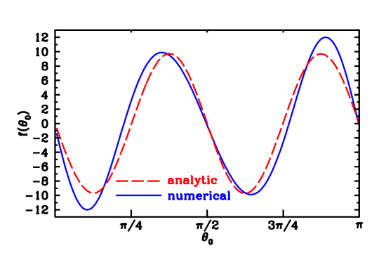
Figure 2: Values of $f(\theta_{0})$ obtained through numerical simulation and using the approximate expression given in Eq. (24) for a value of the symmetry breaking parameter of $x=0.05$ and for a coupling constant $g=0.01$.

Let’s then proceed to compute the power spectrum and the spectral index of the curvature perturbations. It has already been argued that the amplitude $|\delta\theta_{0}(k)|$ can be evaluated at horizon exit. Letting $H_{k}$ be the value of the Hubble parameter when the wavelength $\lambda=2\pi/k$ crossed the Hubble radius during inflation, it is possible to show that for the potential of Eq. (16) the square of the amplitude of the quantum fluctuations is given by

$$|\delta\theta_{0}(k)|^{2}=\frac{H_{k}^{2}}{2k^{3}|\phi|^{2}}\left(\frac{k}{aH}\right)^{2\eta_{1}}\left[1-2x\eta_{1}\cos^{2}(\theta_{0})\ln\left(\frac{k}{aH}\right)\right],$$ (26)

where $\eta_{1}=m^{2}/3H^{2}\ll 1$. Eq. (26) shows that the symmetry breaking induces an very small correction to the ordinary flat power spectrum

$$\mathcal{P}_{\delta\theta_{0}}=\left(\frac{H_{k}}{2\pi|\phi|}\right)^{2}\left(\frac{k}{aH}\right)^{2\eta_{1}}\left[1-2\eta_{1}x\cos^{2}(\theta_{0})\ln\left(\frac{k}{aH}\right)\right].$$ (27)

Now note that the factor $f(\theta_{0})$ is uniquely determined by the initial conditions on the angle and by the specification of the potential. The power spectrum of the curvature perturbations can then be obtained by

$$\mathcal{P}_{\zeta}(k)=\frac{f^{2}(\theta_{0})}{16}\mathcal{P}_{\delta\theta_{0}}(k)=\frac{f^{2}(\theta_{0})}{16}\left(\frac{H_{k}}{2\pi|\phi|}\right)^{2}\left(\frac{k}{aH}\right)^{2\eta_{1}}\left[1-2\eta_{1}x\cos^{2}(\theta_{0})\ln\left(\frac{k}{aH}\right)\right]\approx\frac{f^{2}(\theta_{0})}{16}\left(\frac{H_{k}}{2\pi|\phi|}\right),$$ (28)

where the explicit form obtained for $f(\theta_{0})$ in this case [Eq. (24)] has not been entered for sake of brevity. Eq. (28) then shows that the power spectrum of the curvature perturbations generated through this process is flat to a very good degree. This last aspect can be further stressed by the calculation of the spectral index, which gives

$$n-1=\frac{d\ln\mathcal{P}_{\zeta}}{d\ln k}=2\eta_{1}-\frac{2\eta_{1}x\cos^{2}(\theta_{0})}{1-2\eta_{1}x\cos^{2}(\theta_{0})\ln(k/aH)}\approx 2\left[1-x\cos^{2}(\theta_{0})\right]\frac{m^{2}}{3H^{2}},$$ (29)

thus showing that a very small tilt is induced by the symmetry breaking of the potential and the angle of the background trajectory.

IV Discussion

The analysis of this paper suggests that the production of curvature perturbations due to a broken symmetry of the inflationary potential and the resulting inhomogeneous efficiency of the preheating stage may be a rather common phenomenon. It is, in fact, appropriate to stress that while the magnitude of the curvature perturbations produced through this mechanism will depend on the details chosen for the specific model (potentials, coupling constants, interaction Lagrangians, preheating mechanism, and so forth), the mere fact that the inflationary potential has a minimum characterized by a broken symmetry is sufficient to guarantee the generation of curvature perturbations during the preheating phase. This is because perturbations in a direction orthogonal to the field trajectory yield evolutions of the background that are not just time translations of one other (as would be the case with perturbations along the direction of the trajectory) but that might differ substantially. Such different background evolutions then necessarily lead to different preheating efficiencies, thus resulting in perturbations in the comoving particle number and energy densities.

As it has been shown in Sec. III, choosing a specific preheating model allows one to quantify the magnitude of the curvature perturbations produced by this mechanism and to assess whether these may or may not represent a dominant component with respect to the adiabatic perturbation produced during the slow-roll phase by fluctuations along the radial direction. In the present context, the choice of the instant preheating model of Felder et al. Felder:1998vq has been made because it seems plausible that the preheat field $\chi$ may be coupled to some other fields. Moreover, the nature of such process allows one to obtain convenient analytic estimates of the comoving number density of particles produced that are not affected by the stochasticity, related to the build up of preheat particles, usually present in the standard preheating models Kofman:1997yn . Nonetheless, it seems important to stress that the main conclusions of this work do not depend on the choice of the preheating process, but only on the fact that $n_{\chi}$ depends on the background history, which in turn depends on the initial conditions.

Finally, it seems important to note that if the preheat field is coupled to, and decays into, one single field, then the effect of a broken symmetry of the inflationary potential is to convert isocurvature perturbations into adiabatic perturbations Gordon:2000hv . In this sense, the above model resembles in spirit the curvaton model of Lyth and Wands Lyth:2001nq , but does not require the assumption of an external field.

Appendix A Approximate values of $|\phi_{*}(|\phi_{0}|,\theta_{0};x)|$ and $|\dot{\phi}_{*}(|\phi_{0}|,\theta_{0};x)|$

First consider Eq. (22a). It is straightforward to note that given the inflationary potential, Eq. (16), the exact solution for the background dynamics can be computed once the expansion of the Universe is neglected. The background field dynamics is then given by

$$\phi_{1}(t) = |\phi_{0}|\cos(\theta_{0})\cos(mt),$$ (30a)

$$\phi_{2}(t) = |\phi_{0}|\sin(\theta_{0})\cos\left(\frac{mt}{\sqrt{1+x}}\right).$$ (30b)

Letting $\Delta=\pi x/4$, it is possible to linearize the trajectory by

$$\phi_{1}(t) \approx -|\phi_{0}|\cos(\theta_{0})\sin(\Delta)\lambda$$ (31a)

$$\phi_{2}(t) \approx |\phi_{0}|\sin(\theta_{0})\sin(\Delta)(1-\lambda),$$ (31b)

with $\lambda\in[0,1]$. Then solving for the minimum distance from the origin yields $\lambda=\sin^{2}(\theta_{0})$, which corresponds to a minimum distance $|\phi_{*}|$ of

$$|\phi_{*}|=\frac{|\phi_{0}|\pi x}{2\sqrt{2}}\sin(2\theta_{0}),$$ (32)

where the approximation $\sin(\Delta)\approx\Delta$ has also been used. A plot comparing the analytical approximation obtained in this way with a numerical simulation is shown in Fig. 3.

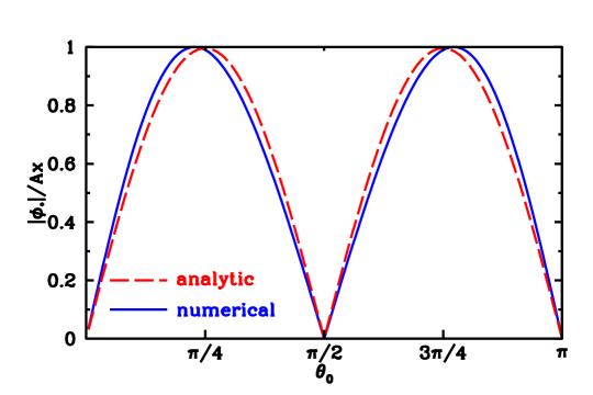
Figure 3: Values of $|\phi_{*}|/(|\phi_{0}|\pi x/2\sqrt{2})$ obtained through numerical simulation and using the above approximate expression Eq. (32) for a value of the symmetry breaking parameter of $x=0.05$.

Not let’s then turn to Eq. (22b). It is a basic fact of a simple harmonic oscillator that $|\dot{\phi}_{*}|=m\Phi$ where $\Phi$ is the amplitude of the oscillation and the mass $m$ is given by the second derivative of the potential along the trajectory

$$m^{2}=\frac{d^{2}V}{dl^{2}}.$$ (33)

Here, $l$ parametrizes the trajectory. To obtain a good estimate for $|\dot{\phi}_{*}|$ let’s first assume that all trajectories pass through the origin. We define

$$m_{1}^{2} = \frac{\partial^{2}V}{\partial\phi_{1}^{2}}=m^{2},$$ (34a)

$$m_{2}^{2} = \frac{\partial^{2}V}{\partial\phi_{2}^{2}}=\frac{m^{2}}{1+x}.$$ (34b)

If the trajectory makes an angle $\beta$ with the $\phi_{1}$ axis, it is then straightforward to show that

$$m_{\beta}^{2}=m_{1}^{2}\cos^{2}(\beta)+m_{2}^{2}\sin^{2}(\beta)=m^{2}\left[\cos^{2}(\beta)+\frac{\sin^{2}(\beta)}{1+x}\right],$$ (35)

which for small value of $x$ reduces to

$$m_{\beta}\approx m\sqrt{1-x\sin^{2}{\beta}}.$$ (36)

Assuming that the trajectory is perfectly radial, which is correct to a good approximation as long as the symmetry breaking parameter $x$ is not too large, then $\beta=\theta_{0}$, and therefore

$$|\dot{\phi}_{*}|\approx|\dot{\tilde{\phi}}_{*}|\sqrt{1-x\sin^{2}{\theta_{0}}},$$ (37)

where $|\dot{\tilde{\phi}}_{*}|=m|\phi_{0}|$ depends only on the initial radial condition. A plot comparing the analytical approximation given by Eq. (36) with numerical simulation is shown in Fig. 4.

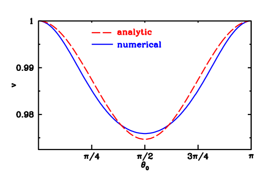
Figure 4: Values of $|\dot{\phi}_{*}|/|\dot{\tilde{\phi}}_{*}|$ obtained through numerical simulation and using the approximate expression Eq. (36) for a value of the symmetry breaking parameter of $x=0.05$.

Appendix B Calculation of the Power Spectrum and the Spectral Index

Start from the fact that

$$\theta = \tan^{-1}\left(\frac{\phi_{2}}{\phi_{1}}\right)$$ (38)

$$\Rightarrow\delta\theta_{0} = \sqrt{\left(\frac{\partial\theta}{\partial\phi_{1}}\right)^{2}\delta\phi_{1}^{2}+\left(\frac{\partial\theta}{\partial\phi_{2}}\right)^{2}\delta\phi_{2}^{2}},$$ (39)

where the two scalar fields are supposed to be uncorrelated. Then for a generic massive scalar field $\sigma_{k}$ we know that on superhorizon scales the amplitude of the quantum fluctuations is given by

$$|\delta\sigma_{k}|\simeq\frac{H_{k}}{\sqrt{2k^{3}}}\left(\frac{k}{aH}\right)^{\frac{3}{2}-\nu_{\sigma}},$$ (40)

where $\nu_{\sigma}^{2}=9/4-m_{\sigma}^{2}/H^{2}$ and it is possible to define the parameter $\eta_{\sigma}=m_{\sigma}^{2}/3H^{2}\simeq 3/2-\nu_{\sigma}$. In our case we have two fields, with masses $m_{\phi_{1}}=m$ and $m_{\phi_{2}}=m/\sqrt{1+x}$. We can then use Eq. (40) to calculate $|\delta\theta_{0}(k)|$ using Eq. (39). However since we’re really interested in computing the power spectrum, we can go directly to its formula, which requires $|\delta\theta_{0}(k)|^{2}$. In general, the power spectrum is defined by

$$\mathcal{P}_{\delta\sigma}\equiv\frac{k^{3}}{2\pi^{2}}|\delta\sigma_{k}|^{2},$$ (41)

so that the first goal of our calculation becomes

$$\mathcal{P}_{\delta\theta}\equiv\frac{k^{3}}{2\pi^{2}}|\delta\theta_{0}(k)|^{2},$$ (42)

but using Eqs. (38, 39) above we then have

$$|\delta\theta_{0}(k)|^{2}=\frac{\phi_{2}^{2}}{|\phi|^{4}}|\delta\phi_{1}|^{2}+\frac{\phi_{1}^{2}}{|\phi|^{4}}|\delta\phi_{2}|^{2}.$$ (43)

Now the only problem is that since the two fields have slightly different masses, we don’t have $|\delta\phi_{1}|=|\delta\phi_{2}|$. Instead

$$|\delta\theta_{0}(k)|^{2}=\frac{H_{k}^{2}}{2k^{3}|\phi|^{2}}\left[\sin^{2}(\theta_{0})\left(\frac{k}{aH}\right)^{2\eta_{1}}+\cos^{2}(\theta_{0})\left(\frac{k}{aH}\right)^{2\eta_{2}}\right],$$ (44)

but

$$\eta_{2}=\frac{m^{2}}{3H^{2}(1+x)}\approx\frac{m^{2}}{3H^{2}}(1-x)=\eta_{1}(1-x),$$ (45)

so that

$$|\delta\theta_{0}(k)|^{2}=\frac{H_{k}^{2}}{2k^{3}|\phi|^{2}}\left(\frac{k}{aH}\right)^{2\eta_{1}}\left[\sin^{2}(\theta_{0})+\cos^{2}(\theta_{0})\left(\frac{k}{aH}\right)^{-2x\eta_{1}}\right].$$ (46)

But recall that $x$ is very small, so that we can use the fact that $a^{x}\approx 1+x\ln(a)$ which then yields

$$|\delta\theta_{0}(k)|^{2}\approx\frac{H_{k}^{2}}{2k^{3}|\phi|^{2}}\left(\frac{k}{aH}\right)^{2\eta_{1}}\left[1-2x\eta_{1}\cos^{2}(\theta_{0})\ln\left(\frac{k}{aH}\right)\right].$$ (47)

We’re now ready to insert this expression in the general definition of the power spectrum and then we get:

$$\mathcal{P}_{\delta\theta} = \frac{k^{3}}{2\pi^{2}}\frac{H_{k}^{2}}{2k^{3}|\phi^{2}|}\left(\frac{k}{aH}\right)^{2\eta_{1}}\left[1-2\eta_{1}x\beta^{2}\ln\left(\frac{k}{aH}\right)\right]$$ (48)

$$= \left(\frac{H_{k}}{2\pi|\phi|}\right)^{2}\left(\frac{k}{aH}\right)^{2\eta_{1}}\left[1-2\eta_{1}x\beta^{2}\ln\left(\frac{k}{aH}\right)\right],$$

We can then note that since $\cos^{2}(\theta_{0})\in[0,1]$ and $x\ll 1$ the spectrum we get is almost flat. Furthermore, the spectral index is given by

$$n-1 = \frac{d\ln\mathcal{P}_{\zeta}}{d\ln k}=2\eta_{1}-\frac{2\eta_{1}x\cos^{2}(\theta_{0})}{1-2\eta_{1}x\cos^{2}(\theta_{0})\ln(k/aH)}$$ (49)

$$\approx 2\eta_{1}\left[1-x\cos^{2}(\theta_{0})\right]=2\left[1-x\cos^{2}(\theta_{0})\right]\frac{m^{2}}{3H^{2}},$$

where the denominator has been approximated to one since the $\eta_{1}x\cos^{2}(\theta_{0})$ term should be very small.

References

- (1) A. Guth, Phys. Rev. D23, 347 (1981)
- (2) D. H. Lyth and A. Riotto, Phys. Rep. 314 1 (1999); A. Riotto, hep-ph/0210162; W. H. Kinney, astro-ph/0301448.
- (3) V. F. Mukhanov and G. V. Chibisov, JETP Lett. 33, 532 (1981).
- (4) S. W. Hawking, Phys. Lett. 115B, 295 (1982).
- (5) A. Starobinsky, Phys. Lett. 117B, 175 (1982).
- (6) A. Guth and S. Y. Pi, Phys. Rev. Lett. 49, 1110 (1982).
- (7) J. M. Bardeen, P. J. Steinhardt, and M. S. Turner, Phys. Rev. D28, 679 (1983).
- (8) W. Hu, arXiv:astro-ph/0402060.
- (9) V. F. Mukhanov, H. A. Feldman and R. H. Brandenberger, Phys. Rept. 215, 203 (1992).
- (10) R. Durrer, arXiv:astro-ph/0402129.
- (11) D. Langlois, arXiv:hep-th/0405053.
- (12) R. H. Brandenberger, Lect. Notes Phys. 646, 127 (2004) [arXiv:hep-th/0306071].
- (13) L. Kofman, A. D. Linde and A. A. Starobinsky, Phys. Rev. D 56, 3258 (1997) [arXiv:hep-ph/9704452].
- (14) G. N. Felder, L. Kofman and A. D. Linde, Phys. Rev. D 59, 123523 (1999) [arXiv:hep-ph/9812289].
- (15) G. Dvali, A. Gruzinov and M. Zaldarriaga, Phys. Rev. D 69, 023505 (2004) [arXiv:astro-ph/0303591].
- (16) G. Dvali, A. Gruzinov and M. Zaldarriaga, Phys. Rev. D 69, 083505 (2004) [arXiv:astro-ph/0305548].
- (17) S. Matarrese and A. Riotto, JCAP 0308, 007 (2003) [arXiv:astro-ph/0306416].
- (18) D. H. Lyth and D. Wands, Phys. Lett. B 524, 5 (2002) [arXiv:hep-ph/0110002].
- (19) A. R. Liddle, D. H. Lyth, K. A. Malik and D. Wands, Phys. Rev. D 61, 103509 (2000) [arXiv:hep-ph/9912473].
- (20) D. Wands, K. A. Malik, D. H. Lyth and A. R. Liddle, Phys. Rev. D 62, 043527 (2000) [arXiv:astro-ph/0003278].
- (21) K. A. Malik, D. Wands and C. Ungarelli, Phys. Rev. D 67, 063516 (2003) [arXiv:astro-ph/0211602].
- (22) S. Gupta, K. A. Malik and D. Wands, Phys. Rev. D 69, 063513 (2004) [arXiv:astro-ph/0311562].
- (23) C. Gordon, D. Wands, B. A. Bassett and R. Maartens, Phys. Rev. D 63, 023506 (2001) [arXiv:astro-ph/0009131].
- (24) See, for instance, R. Kallosh, A. D. Linde, D. A. Linde and L. Susskind, Phys. Rev. D 52, 912 (1995) [arXiv:hep-th/9502069] and references therein.