The Cosmic Evolution of Hard X-ray Selected Active Galactic Nuclei1

Abstract

We use highly spectroscopically complete deep and wide-area Chandra surveys to determine the cosmic evolution of hard X-ray–selected AGNs. For the deep fields, we supplement the spectroscopic redshifts with photometric redshifts to assess where the unidentified sources are likely to lie. We find that the median redshifts are fairly constant with X-ray flux at $z\sim 1$. We classify the optical spectra and measure the FWHM line widths. Most of the broad-line AGNs show essentially no visible absorption in X-rays, while the sources without broad lines (${\rm FWHM}<2000$ km s^-1; “optically-narrow” AGNs) show a wide range of absorbing column densities. We determine hard X-ray luminosity functions for all spectral types with $L_{X}\geq 10^{42}$ ergs s^-1 and for broad-line AGNs alone. At $z<1.2$, both are well described by pure luminosity evolution, with $L_{\ast}$ evolving as $(1+z)^{3.2\pm 0.8}$ for all spectral types and as $(1+z)^{3.0\pm 1.0}$ for broad-line AGNs alone. Thus, all AGNs drop in luminosity by almost an order of magnitude over this redshift range. We show that this observed drop is due to AGN downsizing rather than to an evolution in the accretion rates onto the supermassive black holes.

We directly compare our broad-line AGN hard X-ray luminosity functions with the optical QSO luminosity functions and find that at the bright end they agree extremely well at all redshifts. However, the optical QSO luminosity functions do not probe faint enough to see the downturn in the broad-line AGN hard X-ray luminosity functions and even appear to be missing some sources at the lowest luminosities they probe.

We find that broad-line AGNs dominate the number densities at the higher X-ray luminosities, while optically-narrow AGNs dominate at the lower X-ray luminosities. We rule out galaxy dilution as a partial explanation for this effect by measuring the nuclear UV/optical properties of the Chandra sources using the HST ACS GOODS-North data. The UV/optical nuclei of the optically-narrow AGNs are much weaker than expected if the optically-narrow AGNs were similar to the broad-line AGNs. We therefore postulate the need for a luminosity dependent unified model. An alternative possibility is that the broad-line AGNs and the optically-narrow AGNs are intrinsically different source populations. We cover both interpretations by constructing composite spectral energy distributions—including long-wavelength data from the mid-infrared to the submillimeter—by spectral type and by X-ray luminosity. We use these spectral energy distributions to infer the bolometric corrections (from hard X-ray luminosities to bolometric luminosities) needed to map the accretion history.

We determine the accreted supermassive black hole mass density for all spectral types and for broad-line AGNs alone using the observed evolution of the hard X-ray energy density production rate and our inferred bolometric corrections. We find that only about one-half to one-quarter of the supermassive black hole mass density was fabricated in broad-line AGNs. Using either recent optical QSO luminosity function determinations or our broad-line AGN hard X-ray luminosity function determinations, we measure an accreted supermassive black hole mass density that is a factor of almost two lower than that measured by previous work, assuming $\epsilon=0.1$. This leaves room for the obscured accretion when compared with the local supermassive black hole mass density. In fact, we find reasonable agreement between the accreted supermassive black hole mass density from all spectral types and the local supermassive black hole mass density, assuming $\epsilon\approx 0.1-0.2$. However, there is very little room for further obscured sources or for any low efficiency accretion periods.

1. Introduction

The determination of the time-history of accretion is crucial to our understanding of how supermassive black holes form and evolve. However, much of the accretion power in the universe is absorbed (e.g., Almaini, Lawrence, & Boyle 1999), making it difficult to measure at optical wavelengths. The Chandra (Weisskopf et al. 2002) and XMM-Newton (Jansen et al. 2001) X-ray Observatories have revolutionized distant active galactic nucleus (AGN) studies by making it possible to map the history of the AGN population using hard ($2-8$ keV) X-ray surveys. Hard X-rays can directly probe AGN activity, are uncontaminated by star formation processes at the X-ray luminosities of interest, and detect all but the most absorbed sources. Thus, hard X-ray surveys provide as complete and unbiased a sample of AGNs as is presently possible (e.g., Mushotzky 2004), though they will still miss Compton-thick sources.

Not surprisingly, hard X-ray luminosity functions constructed from Chandra and XMM-Newton samples have revealed that previous optically-selected and soft X-ray–selected AGN samples substantially undercount the AGN population, at least at low and intermediate X-ray luminosities ($L_{2-8~{}{\rm keV}}<10^{44}$ ergs s^-1; Cowie et al. 2003; Hasinger 2003; Steffen et al. 2003; Fiore et al. 2003; Ueda et al. 2003). In fact, optically-selected broad-line AGNs comprise only about a third (e.g., Barger et al. 2003b) of the X-ray background (Giacconi et al. 1962), and many X-ray sources show no signs of AGN activity at all in their optical spectra (e.g., Barger et al. 2001b; Tozzi et al. 2001; Hornschemeier et al. 2001). Theoretical models of supermassive black hole formation (e.g., Haehnelt, Natarajan, & Rees 1998; Kauffmann & Haehnelt 2000, 2002) have historically relied on comparisons with the optical quasar luminosity function, so these models now need to be reworked.

In addition, the hard X-ray luminosity functions have revealed that broad-line AGNs dominate the number densities at the higher X-ray luminosities, while non–broad-line AGNs dominate at the lower X-ray luminosities (Steffen et al. 2003; we hereafter refer to this as the “Steffen effect”). Although we do not yet have a physical explanation for the Steffen effect, there are two simple possibilities to consider. One possibility is that the simple unified model for AGNs, where the differences between broad-line AGNs and non–broad-line AGNs are only due to orientation effects, needs to be modified to include an X-ray luminosity dependent covering factor. The second, more speculative possibility is that the Steffen effect is a consequence of the broad-line AGNs being intrinsically different than the non–broad-line AGNs.

We are now in a position to do a very thorough study of the nature and evolution of hard X-ray–selected AGNs. The primary aims of this paper are to explore the origin of the Steffen effect and to determine the bolometric luminosities of all AGNs in order to understand the energy release history of supermassive black hole accretion. The recent advances that make this comprehensive study possible are the high-resolution, multicolor observations that have been obtained with the ACS camera on the Hubble Space Telescope (HST) of fields with deep Chandra X-ray data, and the extensive, high-quality optical spectroscopic follow-up observations that have been made of X-ray sources detected in both deep and wide-area Chandra surveys.

The structure of the paper is as follows. In §2, we describe the X-ray samples used in our analysis and the completeness of the spectroscopic and photometric redshift identifications. We then determine the X-ray luminosities and median redshifts versus X-ray flux. In §3, we spectrally classify the optical counterparts to the X-ray sources and investigate the dependence of the optical spectral types on X-ray obscuration. In §4, we use multicolor HST ACS Great Observatories Origins Deep Survey (GOODS-North; Giavalisco et al. 2004) observations of the CDF-N to separate the nuclear component of each source from the host galaxy light, and we then compare the (nuclear – galaxy) colors with the optical spectral types.

In §5–§7, we construct up-to-date low and high-redshift hard X-ray luminosity functions (all spectral types and broad-line AGNs alone) for our highly spectroscopically complete samples, do maximum likelihood fits over the redshift range $z=0-1.2$, and examine the evolution of the hard X-ray luminosity functions. In §8, we directly compare the broad-line AGN hard X-ray luminosity functions with the optical QSO luminosity functions. In §9, we determine the evolution of the rest-frame hard X-ray comoving energy density production rate for all spectral types together as well as separated by spectral type. In §10, we estimate black hole masses for a small sample of broad-line AGNs using the measured MgII 2800 Å line widths and nuclear optical luminosities. We then explore “mass starvation” versus “AGN downsizing” as explanations for the observed rapid decline in the energy density production rates between $z=1$ and $z=0$.

We show in §11 that the simple unified model cannot explain the Steffen effect. In §12, we postulate that the simplest interpretation of the Steffen effect is a luminosity dependent unified model, although another interpretation might be intrinsic differences in the source populations. In §13, we discuss how the bolometric corrections to go from X-ray luminosities to bolometric luminosities can be determined. To infer what these corrections are, we need long-wavelength data. In §14, we use mid-infrared (MIR) and far-infrared (FIR)/submillimeter data obtained with the ISOPHOT and ISOCAM instruments on the Infrared Space Observatory (ISO) and the SCUBA bolometer array on the James Clerk Maxwell Telescope (JCMT) to observe directly any enhancements at these wavelengths due to absorption and reradiation by gas and dust. We note that the observational situation in the MIR/FIR may be expected to improve with the Spitzer Space Telescope. Since we do not know for sure what the origin of the Steffen effect is, in §15 and §17, we cover both possibilities (intrinsic differences in the source populations or a luminosity dependent unified model) by constructing composite spectral energy distributions of the sources first by optical spectral type and then by X-ray luminosity. In §16 and §18, we infer the bolometric corrections by spectral type and by X-ray luminosity. In §19, we use our bolometric corrections and the rest-frame hard X-ray comoving energy density production rate to determine the accretion history of the universe. We summarize our results in §20.

We assume $\Omega_{M}=1/3$, $\Omega_{\Lambda}=2/3$, and $H_{o}=65$ km s^-1 Mpc^-1. All magnitudes are in the AB magnitude system.

2. Hard and Soft X-ray Samples

A detailed study of the cosmic evolution of the hard X-ray source population requires the complementarity of deep and wide-field X-ray surveys. Fortunately, both types of X-ray surveys are now becoming available. Since the Chandra angular resolution is critical to the identification of the optical counterparts to the X-ray sources, in this paper we only consider Chandra surveys (except at the very brightest X-ray fluxes, where we supplement our data with an ASCA sample). To make sure our analysis is as robust as possible, we include only the three most spectroscopically complete Chandra surveys available.

The two deep X-ray surveys that we use are the Chandra Deep Field-North (CDF-N) and the Chandra Deep Field-South (CDF-S), the deepest X-ray images ever taken. The $\approx 2$ Ms CDF-N survey samples a large, distant cosmological volume down to very faint X-ray flux limits of $f_{2-8~{}{\rm keV}}\approx 1.4\times 10^{-16}$ ergs cm^-2 s^-1 and $f_{0.5-2~{}{\rm keV}}\approx 1.5\times 10^{-17}$ ergs cm^-2 s^-1 (Alexander et al. 2003b), while the $\approx 1$ Ms CDF-S survey samples only a factor of two shallower (Giacconi et al. 2002).

We supplement these deep surveys with a wide-area, intermediate depth survey in order to sample a large, low-redshift cosmological volume and to detect the rare, high-luminosity population. The low-redshift volume enables us to probe robustly the evolution of AGNs between $z\sim 0$ and $z\sim 1$. The only wide-area, intermediate depth survey published to date that has a high level of spectroscopic completeness is the Chandra Large-Area Synoptic X-ray Survey, or CLASXS. This survey covers an $\sim 0.4$ deg² region in the Lockman Hole-Northwest, imaged to X-ray flux limits of $f_{2-8~{}{\rm keV}}\approx 3\times 10^{-15}$ ergs cm^-2 s^-1 and $f_{0.5-2~{}{\rm keV}}\approx 5\times 10^{-16}$ ergs cm^-2 s^-1 (Yang et al. 2004).

The high spatial resolution of the Chandra X-ray images allows a generally unambiguous optical counterpart to be found for the great majority of X-ray sources having counterparts $R<26$. (Note that about 20% of the optical counterpart identifications in the $R=24-26$ range will be spurious; see §2.3.) Only a few have multiple counterparts. Most of the $R<24$ sources, and many of the $R<25$ sources, can be spectroscopically identified (Barger et al. 2003b; Szokoly et al. 2004; Steffen et al. 2004). In Table 1, we show for the three Chandra fields in our sample (the most intensively spectroscopically observed Chandra fields to date) the total number of sources in the X-ray catalogs, the number of such sources observed spectroscopically, and the number of such sources identified spectroscopically.

If we want to explore the highest X-ray luminosities, we also need much wider-field, higher-flux samples than these Chandra data can provide. ASCA, BeppoSAX, and RXTE provide such samples, but with their low spatial resolutions, cross-identifications to the optical counterparts are more difficult and ambiguous. Ultimately, many of the sources in these surveys will be pinned down with higher resolution Chandra or XMM-Newton observations and their counterparts robustly identified. Fortunately, however, since these high X-ray flux sources generally do have brighter optical counterparts than the sources in lower X-ray flux surveys, in many cases it is already possible to identify the counterparts, even with the positional uncertainties. In particular, the ASCA sample of Akiyama et al. (2003) have nearly complete identifications (see Table 1), albeit with some ambiguous cases, while roughly 70% of the bright RXTE sample have identifications (Sazonov & Revnivtsev 2004).

Hereafter, the CDF-N, CDF-S, CLASXS, and Akiyama et al. (2003) ASCA hard X-ray–selected samples will constitute this paper’s “total hard X-ray sample”, and the CDF-N, CDF-S, and CLASXS soft X-ray–selected samples will constitute this paper’s “total soft X-ray sample”.

Table 1Breakdown of the X-ray Samples by Field and Spectral Class

Category	CDF-N	CDF-S	CLASXS	ASCA
total	503	346	525	32
observed	451	247	467	32
identified	306	137	272	31
broad-line	43	32	106	30
high-excitation	39	23	45	0
star formers	148	55	73	0
absorbers	58	20	28	0
stars	14	7	20	1

2.1. Spectroscopic Completeness

Figure 1 shows the useful flux ranges of the three Chandra surveys and the ASCA survey (which is only in the hard X-ray sample) that make up this paper’s total hard and soft X-ray samples. The surveys provide good coverage over the flux ranges $f_{2-8~{}{\rm keV}}\approx 10^{-16}-10^{-13}$ ergs cm^-2 s^-1 and $f_{0.5-2~{}{\rm keV}}\approx 10^{-17}-10^{-13}$ ergs cm^-2 s^-1. Note that for all of the Chandra surveys, the observed X-ray counts were converted to $2-8$ keV fluxes in the original papers using individual power-law indices determined from the ratios of the hard-to-soft X-ray counts (i.e., the hardness ratios). For the ASCA survey, Akiyama et al. (2003) assumed an intrinsic $\Gamma=1.7$ photon index to compute $2-10$ keV fluxes, so we have converted their $2-10$ keV fluxes to $2-8$ keV assuming their $\Gamma=1.7$.

Figure 2 shows how the contributions to the $2-8$ keV total resolved X-ray background, obtained by extrapolating the number counts to faint and bright X-ray fluxes, are strongly peaked around $f_{2-8~{}{\rm keV}}\approx 10^{-14}$ ergs cm^-2 s^-1. In fact, nearly 75% arises in the $f_{2-8~{}{\rm keV}}\approx 10^{-16}-10^{-13}$ ergs cm^-2 s^-1 range (e.g., Campana et al. 2001; Cowie et al. 2002; Rosati et al. 2002; Alexander et al. 2003b). Approximately 70% of the $2-8$ keV light in the flux range $f_{2-8~{}{\rm keV}}\approx 10^{-16}-10^{-13}$ ergs cm^-2 s^-1 is spectroscopically identified, while about 80% of the $0.5-2$ keV light in the flux range $f_{0.5-2~{}{\rm keV}}\approx 10^{-17}-10^{-13}$ ergs cm^-2 s^-1 is spectroscopically identified.

Figure 1a also shows that the fraction of observed sources that can be spectroscopically identified is a strong function of the hard X-ray flux. Above $f_{2-8~{}{\rm keV}}\approx 10^{-14}$ ergs cm^-2 s^-1, $80-90$% of the sources have spectroscopic redshifts, while below this, the fraction drops to about 60%. While this is partly a consequence of the fainter X-ray sources being optically fainter, it is also a consequence of the fraction of broad-line AGNs being much higher at the brighter X-ray luminosities.

2.2. X-ray Luminosities

The hard X-ray flux limit of $f_{2-8~{}{\rm keV}}\approx 10^{-14}$ ergs cm^-2 s^-1, above which the redshift identifications are very complete ($80-90$%), corresponds to a rest-frame $2-8$ keV luminosity of $L_{X}\approx 5\times 10^{43}$ ergs s^-1 at $z=1$, while the soft X-ray flux limit of $f_{0.5-2~{}{\rm keV}}\approx 2\times 10^{-15}$ ergs cm^-2 s^-1, above which the surveys are about 80% spectroscopically complete, corresponds to a rest-frame $2-8$ keV luminosity of $L_{X}\approx 1.7\times 10^{44}$ ergs s^-1 at $z=3$. Thus, nearly all of the high X-ray luminosity sources have been identified, and incompleteness has very little effect on the bright end of the hard X-ray luminosity function determinations (see §5).

In Figure 3a, we show $2-8$ keV flux versus redshift for the spectroscopically observed sources in the total hard X-ray sample. The CLASXS sources nicely fill in the almost an order of magnitude flux gap between the CDF-N/CDF-S and ASCA samples. The two solid curves correspond to loci of constant rest-frame $2-8$ keV luminosity, $L_{X}$. Any source more luminous than $L_{X}=10^{42}$ ergs s^-1 (lower curve) is very likely to be an AGN on energetic grounds (Zezas, Georgantopoulos, & Ward 1998; Moran, Lehnert, & Helfand 1999), though many of the intermediate luminosity sources do not show obvious AGN signatures in their optical spectra. Sources with $L_{X}>10^{44}$ ergs s^-1 (upper curve) are often called quasars, since this X-ray luminosity roughly corresponds to the absolute optical magnitude of $M_{B}=-23$ that is the traditional dividing line between quasars and Seyfert 1 galaxies. However, the distinction between Seyfert 1 galaxies and quasars seems to have little physical significance. In this paper, we simply refer to all objects which have lines with full width half maximum (FWHM) greater than 2000 km s^-1 in their optical spectra as broad-line AGNs (see §3). The broad-line AGNs are denoted by large symbols in Figure 3a. From the figure, we can see that the great majority of the most luminous sources, where we are very spectroscopically complete, are broad-line AGNs.

In Figure 3b, we show rest-frame $2-8$ keV luminosity versus redshift for the broad-line AGNs alone. At $z<3$, the luminosities were calculated from the observed-frame $2-8$ keV fluxes (squares), and at $z>3$, the luminosities were calculated from the observed-frame $0.5-2$ keV fluxes (diamonds). One advantage of using the observed-frame soft X-ray fluxes at high redshifts is the increased sensitivity, since the $0.5-2$ keV Chandra images are deeper than the $2-8$ keV images. In addition, at $z=3$, observed-frame $0.5-2$ keV corresponds to rest-frame $2-8$ keV, providing the best possible match to the lower redshift data. In calculating the rest-frame luminosities, we have assumed an intrinsic $\Gamma=1.8$, for which there is only a small differential $K$-correction to rest-frame $2-8$ keV. Note that using the individual photon indices (rather than the universal power-law index of $\Gamma=1.8$ adopted here) to calculate the $K$-corrections would result in only a small difference in the rest-frame luminosities (Barger et al. 2002). The curves in Figure 3b show the luminosity limits (using the on-axis flux limits and the $K$-corrections) of the various X-ray surveys used in our analysis. The break in the curves at $z=3$ results from switching from observed-frame $2-8$ keV flux to observed-frame $0.5-2$ keV flux in calculating the rest-frame luminosities (due to the increased sensitivity at $0.5-2$ keV).

We can see the Steffen effect from Figure 3b—the population of broad-line AGNs drops off dramatically at the lower X-ray luminosities. Since broad-line AGNs are straightforward to identify spectroscopically, even in the so-called redshift “desert” at $z\sim 1.5-2$, and since the bulk of the sources in the total X-ray samples have now been spectroscopically observed (see Table 1), we do not need to worry that broad-line AGNs are making up a substantial fraction of the unidentified population. In fact, at $16<R<24$, deep Chandra observations have picked up all of the color-selected quasars identified by the COMBO-17 survey in their fields of view (Wolf et al. 2004). Moreover, deep Chandra observations have picked up all of the spectroscopically identified broad-line AGNs in the highly spectroscopically complete (to $R=24.5$; Cowie et al. 2004b; Wirth et al. 2004) ACS GOODS-North region of the CDF-N (see §3).

At $21<R<25.5$, Steidel et al. (2002) proposed that there might be a subsample of AGNs in their Lyman break galaxy survey that are relatively X-ray faint and hence would not be detected in even the deepest X-ray pointings. They based this on a comparison of the AGNs detected in their Lyman break galaxy survey with the X-ray sources detected in a restricted region of the 1 Ms exposure of the CDF-N. Four of their 148 Lyman break galaxy AGN candidates were detected in X-rays, and two of these were spectroscopically identified. One was found to be an optically-faint broad-line AGN at $z=3.406$. Using their estimated spectroscopic completeness for AGNs and their detection of this one source, they concluded that there could be about 11 such optically-faint broad-line AGNs in a redshift interval of $\Delta z\simeq 0.6$ near $z=3$ in a full Chandra ACIS-I field. As can be seen from Figure 3b, we also easily spectroscopically identified the $z=3.406$ broad-line AGN in the CDF-N, and it does indeed have a low X-ray luminosity. However, other than this one source, the low X-ray luminosity regime at these high redshifts is devoid of broad-line AGNs, despite the X-ray sensitivity to such sources and the ease of spectroscopic identifications of broad-line AGNs. We therefore conclude that there are not very many low X-ray luminosity broad-line AGNs at $z\sim 3$. We will come back to the Steffen effect again when we construct the hard X-ray luminosity functions in §5.

To illustrate the range of luminosities covered by the hard and soft X-ray samples, in Figure 4 we show redshift versus rest-frame (a) $2-8$ keV and (b) $0.5-2$ keV luminosity for the total hard and soft X-ray samples, respectively. Here the rest-frame luminosities of the X-ray sources (squares) were determined from the observed-frame (a) hard and (b) soft X-ray fluxes and the $K$-corrections calculated using a $\Gamma=1.8$ spectrum. The rest-frame luminosity limits of the X-ray surveys (curves) were determined from the on-axis (a) $2-8$ keV and (b) $0.5-2$ keV flux limits of the surveys and the $K$-corrections.

Figure 1.— (a) Spectroscopic completeness (i.e., the fraction of observed sources that are spectroscopically identified) of the hard X-ray surveys that make up the total hard X-ray sample (squares—CDF-N, Barger et al. 2003b; diamonds—CDF-S, Szokoly et al. 2004; triangles—CLASXS, Steffen et al. 2004; circles—ASCA, Akiyama et al. 2003). Sources are grouped into flux bins that increase by a multiplicative factor of 2. Only flux bins containing more than 10 sources are plotted to illustrate the useful flux ranges of the various samples. (b) Same, but now of the soft X-ray surveys that make up the total soft X-ray sample.

Figure 2.— (a) Fraction of the $2-8$ keV light from the X-ray number counts that lies above a given flux for the total hard X-ray sample. Dashed line shows the fraction of the light that is spectroscopically identified. Arrow marks the half-light flux. (b) Same, but now fraction of the $0.5-2$ keV light for the total soft X-ray sample.

Figure 3.— (a) $2-8$ keV flux vs. redshift for the hard X-ray surveys that make up the total hard X-ray sample (squares—CDF-N, Barger et al. 2003b; triangles—CDF-S, Szokoly et al. 2004; diamonds—CLASXS, Steffen et al. 2004; circles—ASCA, Akiyama et al. 2003). Spectroscopically unidentified sources are not shown. Curves correspond to loci of constant rest-frame $2-8$ keV luminosity with $K$-corrections calculated using a $\Gamma=1.8$ spectrum. Lower (higher) curve corresponds to $10^{42}$ ergs s^-1 ($10^{44}$ ergs s^-1). Broad-line AGNs (an optical spectroscopic classification; see §3) are denoted by large symbols. (b) $2-8$ keV luminosity vs. redshift for the broad-line AGNs in the total hard X-ray sample. At $z<3$, the luminosities were calculated from the observed-frame $2-8$ keV fluxes (squares), and at $z>3$, the luminosities were calculated from the observed-frame $0.5-2$ keV fluxes (diamonds). The $K$-corrections were calculated using a $\Gamma=1.8$ spectrum. Curves were determined using the on-axis flux limits of the different surveys and the $K$-corrections (solid—CDF-N, Alexander et al. 2003b; dashed—CDF-S, Giacconi et al. 2002; dotted—CLASXS, Yang et al. 2004; dot-dashed—ASCA, Akiyama et al. 2003). Curves are disjoint at $z=3$, because, as for the individual sources, these luminosities were calculated from the observed-frame $2-8$ keV fluxes for $z<3$ and from the observed-frame $0.5-2$ keV fluxes for $z>3$, and the $0.5-2$ keV Chandra images are deeper than the $2-8$ keV images.

Figure 4.— Rest-frame (a) $2-8$ keV and (b) $0.5-2$ keV luminosity vs. redshift for the total hard and soft X-ray samples, respectively. The luminosities were determined using the observed-frame (a) $2-8$ keV and (b) $0.5-2$ keV X-ray fluxes and $K$-corrections calculated using a $\Gamma=1.8$ spectrum. Spectroscopically unidentified sources and stars are not shown. Broad-line AGNs are denoted by large symbols. Curves were determined using the on-axis (a) $2-8$ keV and (b) $0.5-2$ keV flux limits of the different surveys and the $K$-corrections (solid—CDF-N, Alexander et al. 2003b; dashed—CDF-S, Giacconi et al. 2002; dotted—CLASXS, Yang et al. 2004; dot-dashed—ASCA, Akiyama et al. 2003, only in (a)).

2.3. Photometric Redshifts

It is possible to extend the redshift information to fainter magnitudes using photometric redshifts rather than spectroscopic redshifts, and this has been done for both the CDF-N (Barger et al. 2002, 2003b; P. Capak et al., in preparation) and the CDF-S (Wolf et al. 2004; Zheng et al. 2004). These redshifts are robust and suprisingly accurate (often to better than 8%) for non–broad-line AGNs.

The CDF-N photometric redshifts were computed using broadband galaxy colors and the Bayesian code of Benítez (2000), and only sources with probabilities for the photometric redshift of greater than 90% were included. Zheng et al. (2004) computed their photometric redshifts based on a variety of codes and data sets and included sources with very large offsets from the X-ray positions. However, the positional offsets should not be large, given the accuracy of the Chandra X-ray positions. Moreover, as we move to optically fainter sources, the cross-identifications to the X-ray sources become progressively more insecure. Even with a $2^{\prime\prime}$ match radius, about 20% of optical identifications in the $R=24-26$ range will be spurious, and with larger match radii, many of the identifications will be incorrect (Barger et al. 2003b). Therefore, in our analysis, we only include a CDF-S photometric redshift from Zheng et al. (2004) where the optical counterpart to the X-ray source lies within $2^{\prime\prime}$ of the X-ray position. Despite the different methodologies and the slightly fainter flux limits of the CDF-N, both samples have very similar photometric redshift success rates, with just under 85% of the entire X-ray sample being identified in each of the fields. Treister et al. (2004) claimed that by using the photometric redshifts of Mobasher et al. (2004) for the ACS GOODS-South region of the CDF-S, they could achieve 100% spectroscopic plus photometric redshift completeness in that field. However, Mobasher et al. do not include any photometric redshift reliability measures (like the $>90$% probabilities used in the CDF-N), and hence Treister et al. are likely including photometric redshifts for sources that are really too optically faint for reliable determinations.

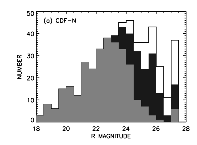
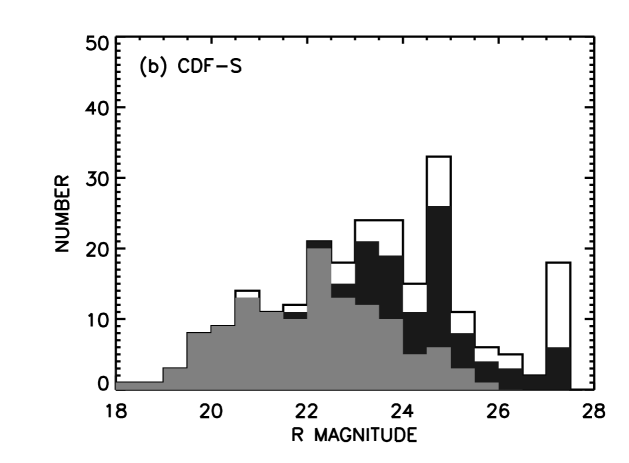
Figure 5.— Fraction of the total (a) CDF-N and (b) CDF-S samples that are spectroscopically (light shading) and photometrically (dark shading) identified vs. $R$ magnitude. All $R>27$ sources are placed in the final magnitude bin. For both samples, the use of photometric redshifts increases the identified fraction to about 85%, with most of the additional identifications lying in the $R=24-26$ magnitude range.

In Figure 2.3, we show the spectroscopic (Barger et al. 2003b; Szokoly et al. 2004) and photometric (Barger et al. 2003b; Zheng et al. 2004) redshift identifications versus $R$ magnitude for the CDF-N and CDF-S. As can be seen from the figure, most sources brighter than $R=24$ can be spectroscopically identified, and photometric redshifts can extend this by almost 2 magnitudes.

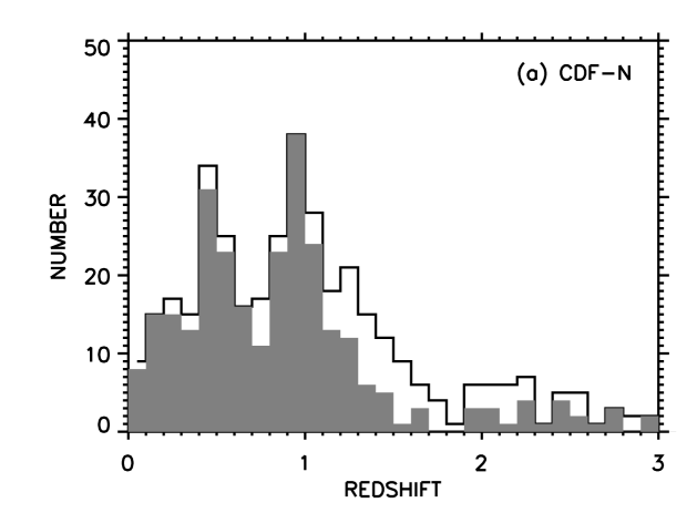
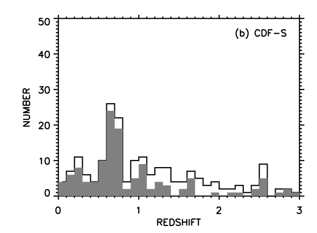
Figure 6.— Fraction of spectroscopically (shading) and photometrically (open histogram) identified sources vs. redshift for the (a) CDF-N and (b) CDF-S samples. As might be expected, the spectroscopic samples are highly complete at $z<1.2$. The spectroscopic incompleteness at $z>1.2$ is due to the absence of strong spectral features and the faintness of the sources at these redshifts, making them harder to identify.

Given the absence, as yet, of a similar set of photometric redshifts for the CLASXS region, we have chosen to analyze our samples primarily by assuming that the redshifts of the optically fainter, spectroscopically unidentified sources are essentially unknown. Nevertheless, we may use the photometric redshifts to assess where the unidentified sources are likely to lie, and hence where incompleteness is likely to be a serious concern in computing the luminosity functions (see §5). We show a comparison of the photometrically identified sources with the spectroscopically identified sources in Figure 2.3. As might be expected, nearly all of the $z<1.2$ sources with photometric redshifts are also spectroscopically identified, and incompleteness only becomes a serious concern at $z>1.2$, where the sources become optically faint and much harder to identify spectroscopically.

Figure 2.3 shows the luminosity versus redshift plot of Figure 4a for just the CDF-N, with the spectroscopic and photometric redshifts denoted by solid and open squares, respectively. Many of the photometrically identified (but spectroscopically unidentified) sources correspond to lower X-ray luminosity sources in the $z=1.2-2.5$ range. We shall assume hereafter that the spectroscopically unidentified sources lie primarily at $z>1.2$.

Figure 7.— Rest-frame $2-8$ keV luminosity vs. redshift for the total hard X-ray sample in the CDF-N. The luminosities were determined using the observed-frame $2-8$ keV fluxes and $K$-corrections calculated using a $\Gamma=1.8$ spectrum. Stars are not shown. Spectroscopically (photometrically) identified sources are denoted by solid (open) squares. Solid curve was determined using the on-axis $2-8$ keV flux limit of the CDF-N survey (Alexander et al. 2003b) and the $K$-corrections.

2.4. Alternate Redshift Estimators

Fiore et al. (2003) have pointed out a correlation between the X-ray–to–optical flux ratios and the hard X-ray luminosities of non–broad-line AGNs, such that higher X-ray luminosity sources tend to have higher X-ray–to–optical flux ratios. This correlation arises due to the obscuration of the nuclear UV/optical light—but not the hard X-ray light—in these systems, such that the host galaxy light dominates. The redshift determination then relies on the fact that the host galaxies have a narrow range in their rest-frame optical magnitudes.

Figure 8.— $f_{X}/f_{R}$ vs. $L_{X}$ for the non–broad-line AGN sample in the CDF-N and CDF-S for $R$-magnitude ranges (a) $R=18-22$, (b) $R=22-24$, and (c) $R=24-26$. Spectroscopic (photometric) redshifts are shown as solid (open) squares. Solid line shows the linear relation given by Fiore et al. (2004).

We can use the spectroscopic plus photometric redshift samples in the CDF-N and CDF-S to test the Fiore et al. (2003) relation. In Figure 2.4, we show the X-ray–to–optical flux ratios versus $L_{X}$ for the non–broad-line AGNs, separated into three $R$ magnitude intervals. Unfortunately, we find that the relationship depends on both variables, with the fainter $R$ magnitude sources having a higher normalization of the X-ray–to–optical flux ratio versus $L_{X}$. This means that applying the Fiore et al. (2003) relation to the sources that do not have redshift determinations (generally because they are faint) using a calibration that is based only on sources with redshifts (generally because they are bright) will result in an overestimate of the redshifts of these sources. Thus, estimates of the number of obscured sources with quasar X-ray luminosities based on this type of analysis will be too high (see, e.g., Padovani et al. 2004).

It might be possible to make a better estimate of the redshifts using the dependence of the rest-frame absolute magnitude on $L_{X}$, together with typical $K$-corrections. However, given the small fraction of unidentified sources in our sample, and the relatively large uncertainties in this type of determination, we do not pursue this in the present paper.

2.5. Median Redshifts

We are now in a position to be able to compare the median redshifts of the total hard and soft X-ray samples at a range of fluxes. In Figure 9, we show spectroscopic redshift distributions for three flux intervals in the total hard X-ray sample. We also show the median redshifts (solid squares) and $1\sigma$ median redshift ranges (solid bars). The $1\sigma$ upper and lower limits on the median redshifts were determined by placing all of the spectroscopically unidentified sources at arbitrarily high and low redshifts, respectively. At the brighter X-ray fluxes, where most of the sources have been spectroscopically identified, the median redshifts are fairly well determined, while at the fainter X-ray fluxes, where the spectroscopic incompleteness is more substantial, the median redshifts are less well determined. In Figure 9c, we also show the median redshift (open square) and $1\sigma$ median redshift range (dotted bars) when we use only the CDF-N and CDF-S data and include the photometric redshifts in the computation, allowing for sources with neither spectroscopic nor photometric redshifts in the same way as above. This substantially improves the accuracy of the median redshift determination in the lowest X-ray flux bin.

Steffen et al. (2004) determined median redshifts for the surveys used in the present paper combined with other ROSAT (Lehmann et al. 2001) and XMM-Newton (Mainieri et al. 2002; Fiore et al. 2003) surveys. Their redshift versus $0.5-2$ keV and $2-8$ keV flux diagrams (their Figures 10a and 10b) showed that the median redshifts of the surveys remained about constant at $z\sim 1$ and were not strongly correlated with either the soft or hard X-ray fluxes. They cautioned, however, that since the magnitudes of high-redshift sources may be faint, the spectroscopic surveys may be biased against finding high-redshift sources, particularly at the fainter X-ray fluxes where the surveys are more incomplete.

We examine this issue in more detail in Figures 10a and 10b, where we show the spectroscopic median redshifts (solid squares) and $1\sigma$ median redshift ranges (solid bars), calculated as in Figure 9, versus $2-8$ keV and $0.5-2$ X-ray flux, respectively, for the total hard and soft X-ray samples. At the lower X-ray fluxes, we also show the median redshifts (open squares) and $1\sigma$ ranges (dotted bars) for the spectroscopic plus photometric CDF-N and CDF-S data. Again we see that the median redshifts of the hard and soft X-ray samples are very similar. Moreover, with the tighter spectroscopic plus photometric median redshift ranges, we see that the median redshifts are indeed fairly constant with flux. The dotted curves show the standard redshift-luminosity relation for a source with rest-frame $2-8$ keV luminosity $L_{X}=10^{44}$ ergs s^-1. The lower X-ray flux sources are clearly dominated by sources with luminosities less than this value and redshifts near one. We shall return to this point when we compute the hard X-ray luminosity functions in §5.

Figure 9.— Spectroscopic redshift distributions for three flux intervals using the total hard X-ray sample. Median redshifts (solid squares) with $1\sigma$ median redshift ranges (solid bars) are also shown. The $1\sigma$ upper and lower limits on the median redshifts were determined by placing all of the unidentified sources at arbitrarily high and low redshifts, respectively. For the lowest flux bin, we also show the median redshift (open square) and $1\sigma$ range (dashed bar) when we use only the CDF-N and CDF-S data and include the photometric redshifts in the computation, placing sources with neither spectroscopic nor photometric redshifts at arbitrarily high and low redshifts, respectively.

Figure 10.— Median redshifts (solid squares) with $1\sigma$ median redshift ranges (solid bars) vs. (a) $2-8$ keV and (b) $0.5-2$ keV flux. The $1\sigma$ upper and lower limits on the median redshifts were determined by placing all of the unidentified sources at arbitrarily high and low redshifts, respectively. For the lower X-ray fluxes, we also show the median redshifts (open squares) and $1\sigma$ ranges (dashed bars) when we use only the CDF-N and CDF-S data and include the photometric redshifts in the computation, placing sources with neither spectroscopic nor photometric redshifts at arbitrarily high and low redshifts, respectively. These have been slightly offset in flux to distinguish them from the spectroscopic points. Dotted curves show the standard redshift-luminosity relation for a source with rest-frame $2-8$ keV luminosity $L_{X}=10^{44}$ ergs s^-1.

3. Optical Spectral Classifications

The optical spectra of the X-ray sources in our sample, while generally of high quality, span different rest-frame wavelengths and suffer varying degrees of AGN mixing with the host galaxy spectrum at different redshifts. It would therefore be quite hard to classify the X-ray sources in any uniform way using a conventional AGN classification scheme. Recognizing this, we have instead only roughly classified the spectroscopically identified Chandra sources into four optical spectral classes. We call sources without any strong emission lines (EW([OII])$<3$ Å or EW(H$\alpha+$NII)$<10$ Å) absorbers; sources with strong Balmer lines and no broad or high-ionization lines star formers; sources with [NeV] or CIV lines or strong [OIII] (EW([OIII] 5007 Å$)>3$ EW(H$\beta)$) high-excitation (HEX) sources; and, finally, sources with optical lines having FWHM line widths $>2000$ km s^-1 broad-line AGNs. We have chosen these four classes to roughly match those used by Szokoly et al. (2004) for the CDF-S (they call the second category low-excitation or LEX sources) in order to combine our own classifications of the CDF-N and CLASXS sources with their classifications of the CDF-S sources. In this paper, we will sometimes combine the absorber and the star former classes into a normal galaxy class.

Table 1 gives the breakdown of the CDF-N, CDF-S, and CLASXS samples by spectral type. Note that four of the CDF-N redshifts are from the literature (see Barger et al. 2003b for references) and hence do not have spectral typings. Hereafter, we call all of the sources that do not show broad-line (FWHM$>2000$ km s^-1) signatures “optically-narrow” AGNs. However, we note that there may be a few sources where our wavelength coverage is such that we are missing lines which would result in us defining the spectrum as broad-line.

For the CDF-N and CLASXS fields, we made a more quantitative analysis by measuring the FWHM line widths for each of the CIV 1550 Å, [CIII] 1909 Å, MgII 2800 Å, H$\beta$, and H$\alpha$ lines that were in the observed spectra by fitting Gaussian profiles to the lines. Where more than one of these lines was within the spectrum, we took the maximum of the measured FWHMs to be the FWHM. There were only significant differences in the measured widths of the various lines for a small number of cases where H$\beta$ was narrow and MgII 2800 Å was wide. For a small number of other spectra, none of the lines were in the observed range, and hence we were not able to classify them. For the cases where the wavelengths of the lines were within our spectra, but no emission lines were visible, we set the widths to zero. Figure 3 shows line width versus optical spectral class for the CDF-N and CLASXS sources.

The choice of 2000 km s^-1 as the dividing line between the high-excitation sources and the broad-line AGNs is in itself rather arbitrary, and many of the sources lying in the high-excitation category would rather naturally fall into the narrow-line Seyfert 1 galaxy definition (Osterbrock & Pogge 1985; Goodrich 1989). To investigate this further, we ran the same classification scheme on the large optical spectroscopic sample given in Cowie et al. (2004b) and Wirth et al. (2004) for the ACS GOODS-North region of the CDF-N field. Figure 3 shows soft X-ray flux versus FWHM line width for these sources. Of the 1718 sources in the GOODS region where we could measure line widths, 20 had FWHM$>800$ km s^-1, and 13 had FWHM$>2000$ km s^-1. All of these sources are X-ray sources.

Figure 11.— FWHM line width vs. optical spectral class for the CDF-N and CLASXS sources. By definition, the broad-line AGNs lie above 2000 km s^-1.

We may make two points from this. First, X-ray–selected samples at the flux limit of the CDF-N essentially find all of the broad-line AGNs. However, some of the intermediate width ($800-2000$ km s^-1) sources would not be found in a field with the CLASXS depth, though they are well above the on-axis CDF-N flux limit. Second, a split at 800 km s^-1 might seem, in some ways, to be more objective than one at 2000 km s^-1.

Figure 12.— $0.5-2$ keV flux vs. FWHM line width for a large, optically-selected sample in the CDF-N (squares). Dashed lines show a FWHM of 800 km s^-1 (vertical) and the CDF-N $0.5-2$ keV flux limit (horizontal). Dotted lines show the minimum FWHM of 2000 km s^-1 for a broad-line source (vertical) and the CLASXS $0.5-2$ keV flux limit (horizontal).

However, when we turn to the X-rays, it is clear that the primary distinction is between the broad-line AGNs and the optically-narrow AGNs. Indeed, this is the only distinction that can easily be made from the X-ray colors or X-ray spectra (Szokoly et al. 2004). In Figure 3, we show the $0.5-2$ keV to $2-8$ keV flux ratio for the sample of sources with strong $2-8$ keV fluxes in the CDF-N and CLASXS fields versus FWHM line width. Above 2000 km s^-1, almost all of the sources are soft ($\Gamma=1.8$), while below this line width, there is a wide span of X-ray colors.

The intermediate width sources show a very similar spread in their X-ray colors relative to all of the remaining optically-narrow sources. This result is consistent with recent work by Williams, Mathur, & Pogge (2004), who used Chandra observations of a sample of optically-selected, X-ray–weak, narrow-line Seyfert 1 galaxies to show that strong, ultrasoft X-ray emission is not a universal characteristic of narrow-line Seyfert 1 galaxies, and, indeed, that many narrow-line Seyfert 1 galaxies have weak or hard X-ray emission.

Figure 13.— $0.5-2$ keV to $2-8$ keV flux ratio vs. FWHM for the sample of sources with $f_{2-8~{}{\rm keV}}>10^{-15}$ ergs cm^-2 s^-1 that lie within 10 arcminutes of the CDF-N aim point, and for the sample of sources with $f_{2-8~{}{\rm keV}}>2\times 10^{-14}$ ergs cm^-2 s^-1 in CLASXS. Horizontal line corresponds to $\Gamma=1.8$. Vertical line corresponds to the mimimum FWHM of 2000 km s^-1 for a broad-line source.

For the CDF-N sources, which have the deepest exposures, we can perform a more sophisticated color analysis. In Figure 3, we show the color-color plot of the $2-4$ keV to $4-8$ keV counts ratio versus the $0.5-2$ keV to $2-8$ keV counts ratio for the $4-8$ keV Chandra sources that have more than 100 counts in that band, separated by optical spectral type (broad-line AGNs in Figure 3a; optically-narrow AGNs in Figure 3b). The broad-line AGNs are nearly all soft with mean photon indices $\Gamma=1.8$ and essentially no visible absorption in X-rays. By contrast, the optically-narrow AGNs are well described by a simple model in which a power-law spectrum with $\Gamma=1.8$ is suppressed at low energies by photoelectric absorption spread over a very wide range of absorbing column densities (Barger et al. 2002; Alexander et al. 2003b). There is little dependence of the absorbing column densities on optical spectral type (shown by the different symbols in Figure 3b) or on the line widths of the optically-narrow AGNs. Thus, the presence of optical Seyfert 2 or narrow-line Seyfert 1 galaxy characteristics does not seem to be dependent on the absorbing column density to the X-ray source.

From Figures 3 and 3, we see that it is possible to separate roughly the broad-line AGNs and the optically-narrow AGNs on the basis of the X-ray colors alone (e.g., Szokoly et al. 2004), without knowing the optical spectra. However, there will be a small amount of contamination from stars, from the small number of optically-narrow AGNs that have soft X-ray colors, and from the small number of broad-line AGNs that have hard X-ray colors. (Note that Perola et al. 2004 found that about 10% of their broad-line AGNs showed some X-ray obscuration, with estimated $N_{H}>10^{22}$ cm^-2.)

Figure 14.— Color-color plot of the $2-4$ keV to $4-8$ keV counts ratio vs. the $0.5-2$ keV to $2-8$ keV counts ratio for the $4-8$ keV sources in the CDF-N 2 Ms exposure with more than 100 counts in the $4-8$ keV band. Curves show a $\Gamma=1.8$ source with absorption from varying column densities. (a) Sources with broad-line optical spectra (“BLAGN”) (large squares) are closely grouped. All but one is consistent with $\Gamma=1.8$ and an effective absorbing column density below $2\times 10^{21}$ cm^-2 (curve is solid above this column density and dotted below). (b) Sources without broad-line optical spectra (“NARROW”) (solid squares—high-excitation signatures; open squares—absorbers and star formers; triangles—unidentified sources) have a wide range of effective column densities, even up to values above $3\times 10^{22}$ cm^-2 (curve is solid above this column density and dotted below).

4. Nuclear UV/Optical Magnitudes

To study the nuclear UV/optical properties of the $2-8$ keV–selected sources, we use multicolor observations of the CDF-N taken with the ACS camera on HST in four bands (ACS F435W, F606W, F814W, and F850LP) as part of GOODS (Giavalisco et al. 2004). (Grogin et al. 2003 used earlier HST observations of the CDF-S for this type of analysis.) Because of the high spatial resolution of these data, we can separate the nuclear component of each source from the host galaxy light, even at the higher redshifts, in order to analyze the nuclear colors. Thus, HST makes it possible for us to reproduce the types of analyses that have been done for decades on low-redshift AGNs and optically-bright AGNs.

Figure 15.— Thumbnail images of sources in the ACS GOODS-North region of the CDF-N at three redshifts: (top panel) $z=0.5$ (F485W), (middle panel) $z=1.0$ (F606W), and (bottom panel) $z=1.5$ (F814W). Each of the three panels contains three separate rows of images: (top row) nucleated, (middle row) somewhat nucleated, (bottom row) no strong nucleus. The sources with spectroscopic typings of broad-line AGN (“BROAD”) or high-excitation (“HEX”) have been labeled as such.

Since the galaxies often have complex morphologies (see Figure 4 for examples), we decided to use a very simple prescription to separate the nuclear magnitudes from the galaxy light. For each source, we first located the peak of the optical light within a $2^{\prime\prime}$ radius around the X-ray position. We then measured the magnitude in a $0.15^{\prime\prime}$ aperture radius centered on this optical position. Based on measurements of 196 spectroscopically confirmed stars in the field, we found that this radius corresponded to the 80 percent enclosed energy fraction. (This is also consistent with the enclosed energy curves in the ACS handbook.) Thus, the $0.15^{\prime\prime}$ aperture magnitude corrected for this enclosed energy fraction provides a first estimate of the nuclear magnitude.

In order to provide an improved estimate of the nuclear magnitude with the galaxy contribution removed, we followed an iterative procedure. We first measured the light within a $0.15^{\prime\prime}-0.3^{\prime\prime}$ annulus around the peak position of the optical light. We then subtracted from this measurement the expected contribution from the nucleus (10% of the $0.15^{\prime\prime}$ radius light, as determined from the PSF) in order to leave only the galaxy contribution. Based on measurements of objects without strong nuclei that otherwise appear to have similar spectral characteristics, we found that the value of the galaxy light in the central $0.15^{\prime\prime}$ radius relative to that in the $0.15^{\prime\prime}-0.3^{\prime\prime}$ annulus is $\sim 0.87$. (We note that this number is rather rough and does not take into account redshift effects.) Thus, we subtracted this estimate of the galaxy light from the $0.15^{\prime\prime}$ aperture magnitude to obtain a revised estimate of the nuclear magnitude. The whole process was then repeated until the estimates converged.

Figure 16.— Rest-frame (nuclear – galaxy) 3000 Å magnitude (computed by interpolating between the GOODS bandpasses) vs. optical spectral type for sources in the ACS GOODS-North region of the CDF-N that lie in the redshift range $z=0.5-2$ and have $L_{X}\geq 10^{42}$ ergs s^-1. For each of the four spectral classes, we show the difference between the nuclear magnitude and the galaxy magnitude of each source in that class (solid diamonds). Sources with (nuclear – galaxy) magnitudes larger than 4.5 or less than $-4.5$ are plotted at these values. The four spectral classes are labeled “ABS” (absorbers), “SF” (star formers), “HEX” (high-excitation sources), and “BLAGN” (broad-line AGNs). All of the broad-line AGNs are strongly nucleated, while almost none of the absorbers or star formers are. Most of the high-excitation sources have comparable nuclear and galaxy magnitudes.

The division between the nucleated sources and those without strong nuclei is generally quite clear. We have illustrated this for three redshifts in Figure 4. Some objects (such as those with double nuclei) can be problematic, but rather than correct these by hand, we have chosen to stay with the objectively measured values. We ran the above procedures on all four color bands in the ACS sample, determining nuclear magnitudes for all 286 objects in the CDF-N 2 Ms list that lie within the GOODS-North region. The galaxy magnitudes are then just the isophotal ACS GOODS-North magnitudes minus the nuclear magnitudes.

There is a good correlation between the fraction of nuclear UV light in the galaxy and the optical spectral type, which gives us confidence in the procedure, since these are completely independently measured properties. In Figure 4, we show nuclear UV magnitude minus galaxy magnitude for all of the X-ray sources versus optical spectral type. The broad-line AGNs and the stars are all strongly nucleated, while the absorbers and star formers have much weaker nuclei, and the high-excitation sources lie at intermediate values.

Of the 286 sources measured, 130 have no detectable nucleus in the $B$-band, and 126 have no detectable nucleus in the $z^{\prime}$-band. Only 4 of the sources without nuclei are spectrally classified as high-excitation sources, and none are classified as broad-line AGNs.

5. Low-Redshift Hard X-ray Luminosity Functions

With the advent of the Chandra and XMM-Newton data, there have been several computations of the evolution of the hard X-ray luminosity functions with redshift (e.g., Cowie et al. 2003; Hasinger 2003; Steffen et al. 2003; Ueda et al. 2003; Fiore et al. 2003). It is a measure of how rapidly the science is evolving that the Chandra spectroscopic samples are now much improved over those used in even these recent calculations. The Chandra samples of Table 1 now contain 1165 spectroscopically observed sources and 715 spectroscopically identified sources.

In calculating the hard X-ray luminosity functions, we use only the spectroscopically observed sources. This approach is strictly valid for CLASXS and the CDF-S, where the X-ray sources were randomly observed. For the CDF-N, there may be a small bias since the spectroscopy does not come purely from targeted observations of the X-ray sample. However, as there are now only 52 X-ray sources in the CDF-N that have not been observed, it would make very little difference to the results if we were instead to use all of the sources.

There are a total of 698 spectroscopically observed sources in the CDF-N and CDF-S samples. Of these, 601 have either spectroscopic or photometric redshifts. We can test for the effects of incompleteness in our analysis by using the spectroscopic plus photometric redshifts in these two fields and the spectroscopic redshifts for the ASCA data, where only one source is unidentified.

Here we recompute the hard X-ray luminosity functions following Cowie et al. (2003), who used the traditional $1/V_{a}$ method of Felten (1977). We use the spectroscopically observed samples of Table 1. We define the hard X-ray luminosity function versus rest-frame $2-8$ keV X-ray luminosity and redshift, $d\Phi(L_{X},z)/{d\log L_{X}}$, as the number of X-ray sources per unit comoving volume per unit base 10 logarithmic luminosity that lie in the redshift interval. We determine the solid angle covered by the observed sources at a given flux by comparing the observed number of sources versus flux with the averaged number counts in the appropriate energy band from Cowie et al. (2002) and Yang et al. (2004). This method allows a simple treatment of the incompleteness that was modeled in computing the counts. However, the counts in Cowie et al. also include the low CDF-S counts, which may affect the normalization at the 10% level relative to the CLASXS average (Yang et al. 2004). We consider this to be a reasonable estimate of the systematic errors. At $10^{-14}$ ergs cm^-2 s^-1 ($2-8$ keV), where the contribution to the $2-8$ keV X-ray background peaks (see §2.1), the solid angle is dominantly from CLASXS. In Figure 5, we show solid angle versus (a) $2-8$ keV and (b) $0.5-2$ keV flux for the observed hard and soft X-ray samples, respectively.

Figure 17.— Solid angle vs. (a) $2-8$ keV and (b) $0.5-2$ keV flux for the observed hard and soft X-ray samples, respectively.

In Figures 18a, 18b, and 18c, we show the hard X-ray luminosity functions for all spectral types (squares; this includes all of the spectroscopically identified X-ray sources with $L_{X}\geq 10^{42}$ ergs s^-1, without regard to the optical spectroscopic classifications) and for broad-line AGNs (diamonds; this includes all of the spectroscopically identified broad-line AGNs) for three low-redshift intervals. These hard X-ray luminosity functions were computed from the observed-frame $2-8$ keV measurements, assuming an intrinsic $\Gamma=1.8$. The Poissonian $1\sigma$ uncertainties are based on the number of galaxies in each luminosity bin. At these low redshifts, there is relatively little uncertainty from incompleteness, since the sources have X-ray fluxes lying in the range where most sources are spectroscopically identified. The triangles show the values computed for what we hereafter refer to as the “spectroscopic plus photometric” sample. For this sample, we consider only the CDF-N, CDF-S, and ASCA spectroscopically observed sources and assign CDF-N and CDF-S photometric redshifts, where available, to those sources that are spectroscopically unidentified. The resulting identified sample is therefore a combination of spectroscopic and photometric redshifts. Note that because this sample does not contain the CLASXS data, in some cases the values (triangles) lie below the spectroscopic values (squares) due to poor sampling by the deep fields of the low-redshift volume and of the high-luminosity sources. In Figure 18d, we show the local $3-20$ keV luminosity function from the RXTE analysis of Sazonov & Revnivtsev (2004).

The forms of the hard X-ray luminosity functions for all spectral types and for broad-line AGNs are clearly very different. The hard X-ray luminosity functions for broad-line AGNs peak at a characteristic luminosity, such that the dominant population at the higher X-ray luminosities is broad-line AGNs, while the dominant population at the lower X-ray luminosities is optically-narrow AGNs. This reproduces the Steffen effect discussed in §2.2. We show this more clearly in Figure 19, where we plot the ratio (squares) of the hard X-ray luminosity functions for all spectral types to the hard X-ray luminosity functions for broad-line AGNs. Above $L_{X}=10^{44}$ ergs s^-1, the fraction of sources that are broad-line AGNs is very high, while below $L_{X}=10^{43}$ ergs s^-1, the fraction of sources that are broad-line AGNs is very low. This result still holds when we include in the hard X-ray luminosity functions for all spectral types all of the spectroscopically unidentified sources. This is done by placing the unidentified sources at the center of each redshift interval and then including them in the luminosity bin where their luminosities at that redshift would put them (dashed curves). Thus, we have clearly detected a luminosity dependence in optical spectral type.

In Figures 18e–g, we show the division between the optically normal galaxies (our absorber and star former classes) and the sources which show clear AGN signatures in their optical spectra (our high-excitation and broad-line AGN classes). Including the high-excitation sources slightly raises the normalization of the broad-line AGN luminosity function, but it does not change its shape much. At low X-ray luminosities, the optically normal galaxies comprise nearly the entire population. The cross-over point lies around $L_{X}<10^{43}$ ergs s^-1 at $z=0.25$ and rises to $L_{X}<10^{44}$ ergs s^-1 near $z=1$. All of the curves in Figure 18 show pure luminosity evolution in both the luminosity functions and the spectral type mix. This must be understood in any model that seeks to explain the difference between the optically normal galaxies and those with AGN characteristics in their optical spectra. This type of parallel evolution is probably most easily understood for a luminosity dependent unified model (see §12).

6. Evolution of the Low-Redshift Hard X-ray luminosity functions

The low-redshift hard X-ray luminosity functions are well represented (solid and dashed curves; Figure 18) by a conventional double power-law fit (Piccinotti et al. 1982) of the form

$${{d\Phi(L_{X},z)}\over{d\log L_{X}}}={a\over{(L/L_{\ast})^{g1}+(L/L_{\ast})^{g2}}}\,.$$ (1)

Parameterizing the redshift evolution as

$$L_{\ast}=L_{0}\Bigl{(}{{1+z}\over 2}\Bigr{)}^{A}\,$$ (2)

and

$$a=a_{0}\Bigl{(}{{1+z}\over 2}\Bigr{)}^{B}\,,$$ (3)

we determined the six parameters and their $1\sigma$ uncertainties for both the hard X-ray luminosity function for all spectral types and the hard X-ray luminosity function for broad-line AGNs using maximum likelihood fits over the redshift range $z=0-1.2$ (Cash 1979; Marshall et al. 1983). The parameters are summarized in Table 2. The evolution of both hard X-ray luminosity functions is consistent with pure luminosity evolution—as is the evolution of the hard X-ray luminosity function for optically-selected broad-line AGNs (Boyle et al. 2000)—where the values of $g1$, $g2$, and $a$ remain constant and only $L_{\ast}$ evolves. The fits are acceptable throughout the redshift range, as shown in Figures 18a–d.

Table 2Maximum Likelihood Fit Parameters for All Spectral Types and for Broad-line AGNs

Parameter	All	Broad-line
$\log L_{0}$	$44.11\pm 0.08$	$43.81\pm 0.12$
$\log a_{0}$	$-4.42\pm 0.07$	$-4.44\pm 0.14$
$g_{1}$	$0.42\pm 0.06$	$-0.9\pm 0.5$
$g_{2}$	$2.2\pm 0.5$	$1.6\pm 0.3$
$A$	$3.2\pm 0.8$	$3.0\pm 1.0$
$B$	$-0.1\pm 0.7$	$-0.1\pm 0.6$

The above fit to the hard X-ray luminosity function for all spectral types agrees well with that of Ueda et al. (2003) at higher luminosities but is shallower below the break, where Ueda et al. find $g1=0.82\pm 0.13$ for their pure luminosity evolution model. In fact, the Ueda et al. slope overpredicts our low-luminosity counts throughout the $z=0-1.2$ redshift range. Our data sample is much larger than the sample used in Ueda et al., particularly in this redshift range, because of our inclusion of the wide-field CLASXS data; correspondingly, our fit should be more robust.

Our $L_{\ast}=(1+z)^{3.2\pm 0.8}$ evolution at $z<1.2$ is steeper than the $L_{\ast}\sim(1+z)^{2.7}$ evolution found by Ueda et al. (2003), though consistent within the uncertainties. Sazonov & Revnivtsev (2004) found that the Ueda et al. (2003) model lay significantly above their local determination. In contrast, our steeper luminosity evolution matches the Sazonov & Revnivtsev (2004) local determination within the uncertainties in the determination of the $A$ parameter (see Figure 18d).

Thus, AGNs drop in luminosity by almost an order of magnitude over the $z=0-1$ redshift range. This drop applies equally to all AGNs, regardless of optical spectral type. We shall return to the question of whether this is an evolution of the accretion rate or of the active population of supermassive black holes in §10.

Figure 18.— Rest-frame $2-8$ keV luminosity function per unit (base 10) logarithmic luminosity in the redshift intervals (a) $z=0.8-1.2$, (b) $z=0.4-0.8$, and (c) $z=0.1-0.4$. Hard X-ray luminosity functions for all spectral types (broad-line AGNs) are denoted by squares (diamonds) and were computed from the observed-frame $2-8$ keV data. We assumed an intrinsic $\Gamma=1.8$, for which there is only a small differential $K$-correction to rest-frame $2-8$ keV. Poissonian $1\sigma$ uncertainties are based on the number of sources in each luminosity bin. Triangles denote the spectroscopic plus photometric hard X-ray luminosity functions, which use only the CDF-N, CDF-S, and ASCA data (see text for details). (d) Local hard X-ray luminosity function determined by Sazonov & Revnivtsev (2004) using RXTE data, shown with (upper dotted curve) and without (lower dotted curve) their assumed incompleteness correction of 1.4. These curves are also shown in the other panels. Solid (dashed) curves show the maximum likelihood fit to the hard X-ray luminosity function for all spectral types (broad-line AGNs) computed at the geometric mean for each redshift interval. Only the maximum likelihood fit to the hard X-ray luminosity function for all spectral types computed at $z=0$ is shown in (d).

Figure 18.— (continued) Parts (e)–(g) show the same redshift intervals as (a)–(c), but now the open squares denote optically normal galaxies alone, and the open diamonds denote high-excitation sources and broad-line AGNs together. The solid and dashed lines are the same as in (a)–(c). The optically normal galaxies dominate the populations at low X-ray luminosities, while the inclusion of the high-excitation sources only slightly increases the broad-line AGN luminosity functions.

Figure 19.— Ratio (squares) of the rest-frame $2-8$ keV luminosity function per unit logarithmic luminosity in the redshift intervals (a) $z=0.8-1.2$, (b) $z=0.4-0.8$, and (c) $z=0.1-0.4$ for all spectral types (squares from Figures 18a–c) relative to that for broad-line AGNs (diamonds from Figures 18a–c). Dashed curves show the same ratio, but with all of the spectroscopically unidentified sources in the spectroscopically observed sample included in the hard X-ray luminosity functions for all spectral types. This was done by placing the unidentified sources at the center of each redshift interval and then including them in the luminosity bin where their luminosities at that redshift would put them. Uncertainties are $1\sigma$ based on the number of sources in each bin.

Figure 20.— Rest-frame $2-8$ keV luminosity function per unit logarithmic luminosity in the redshift intervals (a) $z=1.5-3$ and (b) $z=3-5$. Hard X-ray luminosity functions for all spectral types (broad-line AGNs) are denoted by squares (diamonds) and were computed from the observed-frame $0.5-2$ keV data. Poissonian $1\sigma$ uncertainties are based on the number of sources in each luminosity bin. Dot-dashed curves are the maximal hard X-ray luminosity functions for all spectral types in each redshift interval. These were found by assigning redshifts at the center of each redshift interval to all of the spectroscopically unidentified sources in the spectroscopically observed sample. Triangles denote the spectroscopic plus photometric hard X-ray luminosity functions, which use only the CDF-N, CDF-S, and ASCA data (see text for details). Solid (dashed) curves denote the maximum likelihood fit to the $z=0-1.2$ hard X-ray luminosity function for all spectral types (broad-line AGNs) computed at $z=1$.

7. High-Redshift Hard X-ray Luminosity Functions

We also determined the hard X-ray luminosity functions for two high-redshift intervals, $z=1.5-3$ and $z=3.0-5.0$, using a $0.5-2$ keV observed-frame sample to provide the best possible match to the lower redshift data. Figures 20a and 20b show these measured hard X-ray luminosity functions (squares—all spectral types; diamonds—broad-line AGNs). It is very difficult to measure host galaxy redshifts for sources that lie in the high-redshift intervals, so incompleteness is potentially a large source of error. We therefore computed maximal hard X-ray luminosity functions for all spectral types by assigning redshifts at the center of each redshift interval to all of the spectroscopically unidentified sources (i.e., we included all of the unidentified sources in both redshift intervals). We show these as dot-dashed curves in the figures. It is important to keep in mind that because all of the unidentified sources have been included in both redshift intervals (provided that the sources, when assigned those redshifts, are at $L_{X}\geq 10^{42}$ ergs s^-1), the curves are not consistent with one another. Because the spectroscopic identifications are much more complete at higher X-ray fluxes, the associated systematic uncertainties are larger at lower $L_{X}$. (Note that any low X-ray flux source assigned to a given redshift interval will have a low $L_{X}$ in that redshift interval.) We also show as triangles the spectroscopic plus photometric hard X-ray luminosity functions determined from the CDF-N, CDF-S, and ASCA data only. In the $z=1.5-3$ redshift interval, the spectroscopic plus photometric hard X-ray luminosity function is much closer to the maximal hard X-ray luminosity function than is the spectroscopic hard X-ray luminosity function, whereas in the $z=3-5$ redshift interval, the spectroscopic plus photometric hard X-ray luminosity function is very similar to the spectroscopic hard X-ray luminosity function. This suggests that many of the spectroscopically unidentified sources lie in the $z=1.5-3$ interval rather than at higher redshifts.

Even with our maximal incompleteness corrections, at $L_{X}<10^{44}$ ergs s^-1, the hard X-ray luminosity functions for all spectral types in the two high-redshift intervals lie below the maximum likelihood fits to the $z=0-1.2$ hard X-ray luminosity function computed at $z=1$ (solid curve), suggesting a peak in the universal AGN energy density production rate near $z=1$. However, at $L_{X}>10^{44}$ ergs s^-1, the maximal hard X-ray luminosity functions in both high-redshift intervals appear to continue the increasing trend with redshift.

Before proceeding, we want to make sure that we would not have gotten different results if we had used the $2-8$ keV observed-frame sample instead of the $0.5-2$ keV observed-frame sample in determining the high-redshift hard X-ray luminosity functions. We performed this check by computing the $z=1.5-3$ hard X-ray luminosity function for broad-line AGNs using the $0.5-2$ keV observed-frame sample and also using the $2-8$ keV observed-frame sample. In Figure 7, we show that the agreement between these two computations is very good.

Figure 21.— Hard X-ray luminosity function for broad-line AGNs at $z=1.5-3$ computed from the observed-frame $0.5-2$ keV (diamonds) and observed-frame $2-8$ keV (squares) samples. Dashed curve denotes the maximum likelihood fit to the $z=0-1.2$ hard X-ray luminosity function for broad-line AGNs computed at $z=1$.

8. Comparison with Optical QSO Luminosity Functions

Since the X-ray–selected broad-line AGNs recover essentially all of the optically-selected type 1 AGNs (see §3), we should be able to compare directly the broad-line AGN hard X-ray luminosity functions computed above with the optical QSO luminosity functions. In order to compare the two, we calculate the bolometric luminosities using the bolometric corrections determined by Elvis et al. (1994) (i.e., $L_{BOL}=35\times L_{X}$ for the broad-line AGN hard X-ray luminosity functions, and $L_{BOL}=11.8\nu_{B}L_{\nu_{B}}$ for the QSO luminosity functions). In Figure 22, we show for six redshift intervals the broad-line AGN hard X-ray luminosity functions (open diamonds) and the rest-frame $B$-band QSO luminosity functions (Croom et al. 2004; solid squares) versus the calculated bolometric luminosities. The Croom et al. luminosity functions have been renormalized to our assumed geometry.

The bright end luminosity functions agree extremely well at all redshifts, confirming that the two methodologies are measuring the same sample and that the bolometric corrections used are appropriate. The optical QSO luminosity functions do not probe faint enough to see the downturn in the broad-line AGN hard X-ray luminosity functions. Moreover, they may be missing some sources at the very lowest luminosities to which they probe, as can be seen from the lowest redshift panels.

The optical QSO luminosity function in the $M_{B}=-23$ to $-26$ range is well described by pure luminosity evolution over the redshift range $z=0.3-2.1$ (Boyle et al. 2000). Croom et al. (2004) parameterize this as $L$ evolving as $10^{k1z+k2z^{2}}$, where $k1=1.39$ and $k2=-0.29$. In Figure 8, we compare the Croom et al. evolution with the $(1+z)^{3.0}$ law we determined in §6 for the broad-line AGNs (see Table 2). The Croom et al. evolution is slightly steeper, though part of the difference may lie in the adopted functional forms and in the different redshift ranges over which the laws have been fitted. However, within the uncertainties, the two determinations are consistent over the $z=0-1.2$ redshift interval.

We further investigate the pure luminosity evolution model for broad-line AGNs by using the Croom et al. (2004) evolution law (which was fit over a wider redshift range, $z=0.3-2.1$, than our maximum likelihood fit was, $z=0-1.2$) to correct all of the X-ray luminosities to their values at $z=1$. We then compute the hard X-ray luminosity functions for broad-line AGNs over the wide redshift ranges $z=0.2-0.7$, $z=0.7-1.5$, and $z=1.5-2.5$. The resulting hard X-ray luminosity functions are compared in Figure 8. The lower redshift functions (open triangles and open diamonds) match each other and our maximum likelihood fit computed at $z=1$ (dashed curve) throughout the luminosity range, while the highest redshift function (solid squares) matches the lower redshift functions and our maximum likelihood fit only at the bright end, where the optical QSO determinations are made. It is clear that there are fewer intermediate luminosity sources in the highest redshift interval, and hence that the pure luminosity evolution model cannot in fact be carried reliably to the higher redshifts. This is another statement that the lower luminosity sources peak in number at lower redshifts than the high-luminosity sources (e.g., Cowie et al. 2003; Hasinger 2003; Barger et al. 2003a; Steffen et al. 2003; Fiore et al. 2003; Ueda et al. 2003).

Figure 22.— Open diamonds show the rest-frame $2-8$ keV luminosity function per unit (base 10) logarithmic luminosity for the broad-line AGNs vs. bolometric luminosity ($L_{BOL}=35\times L_{X}$) in the redshift intervals (a) $z=0.28-0.8$, (b) $z=0.6-1.06$, (c) $z=0.8-1.42$, (d) $z=1.2-1.58$, (e) $z=1.51-1.83$, and (f) $z=1.7-2.21$. Solid squares show the rest-frame $B$-band luminosity function of Croom et al. (2004) vs. bolometric luminosity ($L_{BOL}=11.8\nu_{B}L_{\nu}(B)$) in the redshift intervals (a) $z=0.40-0.68$, (b) $z=0.68-0.97$, (c) $z=0.97-1.25$, (d) $z=1.25-1.53$, (e) $z=1.25-1.53$, and (f) $z=1.81-2.10$ adapted from their Table 4.

Figure 23.— Evolution with redshift of the normalizing luminosity in the pure luminosity evolution models for the broad-line AGN hard X-ray luminosity function (dashed line) and the optical QSO luminosity function (solid line). Both have been normalized to unity at $z=1$ and are shown only over the fitted ranges.

Figure 24.— Broad-line AGN hard X-ray luminosity functions (open triangles—$z=0.2-0.7$; open diamonds—$z=0.7-1.5$; solid squares—$z=1.5-2.5$) with luminosities normalized to the values at $z=1$ using the pure luminosity evolution model of Croom et al. (2004). Dashed curve shows the maximum likelihood fit to the $z=0-1.2$ hard X-ray luminosity function for broad-line AGNs (see §6) computed at $z=1$.

9. Hard X-ray Energy Density Production Rate

In Figure 9, we show the evolution with redshift of the $2-8$ keV comoving energy density production rate, ${\dot{\lambda}_{X}}$, of all spectroscopically identified $L_{X}\geq 10^{42}$ ergs s^-1 AGNs (solid squares) and broad-line AGNs alone (open diamonds). The production rate rises rapidly from $z=0$ to $z=1$. The solid and dashed curves show the $(1+z)^{3.2}$ and $(1+z)^{3.0}$ laws found for all spectral types and for broad-line AGNs alone, respectively, in §6. There is no reason why the evolution should be well fitted by a power of $(1+z)$, and, indeed, at $z>1$, the evolution is turning over in redshift, at least in part due to incompleteness. If we had instead fitted over a lower redshift range (say $z=0$ to $z=1$), then we would have obtained a slightly steeper relation.

Such an extremely rapid evolution with redshift bears a striking resemblance to the overall redshift evolution of the star formation rate density in $z<1$ galaxies. The UV luminosity density in small star-forming galaxies is falling as $(1+z)^{1.7\pm 1.0}$ (Wilson et al. 2002; note that there have been a whole slew of relations determined, including some that are steeper). However, AGNs are more likely to be related to the bulge luminosity of galaxies, and hence to the submillimeter and ultraluminous infrared galaxy $(L_{FIR}>10^{12}~{}{\rm L}_{\odot})$ populations. The evolution of the star-forming luminosity function at $z=0.5-1.5$, as determined from radio sources with the equivalent radio power of at least $L_{FIR}=10^{12}~{}{\rm L}_{\odot}$, is steeper and reasonably well described by a $(1+z)^{3.8}$ evolution (Cowie et al. 2004a).

Figure 25.— Evolution with redshift of the rest-frame $2-8$ keV comoving energy density production rate, ${\dot{\lambda}_{X}}$, of all spectroscopically identified $L_{X}\geq 10^{42}$ ergs s^-1 AGNs (solid squares). Open diamonds show the values for broad-line AGNs. Open squares show the maximal incompleteness found by assigning redshifts at the center of each high-redshift interval to all of the spectroscopically unidentified sources in the spectroscopically observed samples. Maximal incompleteness values are not consistent with one another, because all of the unidentified sources are included in both redshift intervals, provided that the sources, when placed at those redshifts, lie at $L_{X}\geq 10^{42}$ ergs s^-1. Curves show the pure luminosity evolution maximum likelihood fits for all spectral types (solid) and for broad-line AGNs alone (dashed) over the range $z=0-1.2$, where $L_{\ast}=(1+z)^{3.2}$ and $L_{\ast}=(1+z)^{3.0}$, respectively.

The peak of the hard X-ray energy density production rate of all spectroscopically identified $L_{X}\geq 10^{42}$ ergs s^-1 AGNs is in the interval $z=0.8-1.2$ and is about $4.6\times 10^{39}$ ergs s^-1 Mpc^-3. About one-third of this production arises in broad-line AGNs and about two-thirds in optically-narrow AGNs. Half of this production arises in sources more luminous than $8.2\times 10^{43}$ ergs s^-1, where the majority of the sources are broad-line AGNs.

The above results are based on direct summation over the individual sources, but integration of the power-law fits to the hard X-ray luminosity functions give similar answers. The largest uncertainty is the redshift distribution of the spectroscopically unidentified sources, not the small effects of extrapolation outside of the observed luminosity range.

In Figure 9, we assume that most of the spectroscopically unidentified sources in the spectroscopically observed samples lie at $z>1.5$ (we examine this in more detail below). We then determine the maximal incompleteness for the two high-redshift intervals (open squares) by using the sources that have a measured spectroscopic redshift in these intervals and by assigning redshifts at the center of each interval to all of the spectroscopically unidentified sources in the spectroscopically observed samples. Note that the maximal incompleteness values are not consistent with one another, because all of the unidentified sources are included in both redshift intervals, provided that the sources, when placed at those redshifts, lie at $L_{X}\geq 10^{42}$ ergs s^-1. Even with the incompleteness uncertainty, ${\dot{\lambda}_{X}}$ is at most flat beyond $z=1$.

To explore more carefully the incompleteness at all redshifts, in Figure 9, we show the production rate for the spectroscopic samples in the CDF-N, CDF-S, and ASCA fields only (solid squares), and, at $z<1.5$, the production rate for the spectroscopic plus photometric samples in these fields (triangles). We see that the only substantial difference at $z<1.5$ is in the $z=1.1-1.5$ redshift interval. At $z=1$, the symbols are a bit higher than the solid square was in Figure 9 (the solid curve from Figure 9 has been replotted in Figure 9 to illustrate this) because of the excess in the CDF-N at that redshift, which gets smoothed out when the CLASXS data are included. We compute the maximal incompleteness for the two high-redshift intervals (open squares) by using the sources with either a spectroscopic or photometric redshift in these intervals and by assigning redshifts at the center of each interval to all of the remaining unidentified sources in the CDF-N, CDF-S, and ASCA fields. The inclusion of the photometric data does not change the conclusion that at $z>1$, ${\dot{\lambda}_{X}}$ is flat or, more realistically, slightly falling.

We can go one step further in studying the evolution of the energy density production rate. In Figure 9, we separate out the optically-narrow AGNs (solid circles), incompleteness correct their production rates (see below), and then compare the evolution of their corrected production rates with the evolution of the production rates of the broad-line AGNs (open diamonds; values from Figure 9). Over the redshift range $z=0-1.5$, the incompleteness corrections were obtained by multiplying the spectroscopically identified optically-narrow AGNs by the ratios of the spectroscopic plus photometric values in Figure 9 (the triangles in that figure) to the spectroscopic values in Figure 9 (the solid squares in that figure). At $z<1.5$, the only place where the incompleteness corrections are significant is in the redshift interval $z=1.1-1.5$.

For $z=1.5-3$, we cannot incompleteness correct so simply. Instead, we compute the possible range of values (vertical bar) by subtracting the value given in Figure 9 for broad-line AGNs (the diamond at $z=1.5-3$) from the value given in Figure 9 for all spectral types (the solid square at $z=1.5-3$) to get the lower value (solid circle), and by subtracting the same value for broad-line AGNs from the value given in Figure 9 for the maximal incompleteness (the open square at $z=1.5-3$) to get the upper value (open circle).

From Figure 9, we conclude that at $z<1$, most of the hard X-ray energy density production is coming from optically-narrow AGNs, while at higher redshifts, this reverses, and the broad-line AGNs dominate the production, even with the maximal incompleteness. The broad-line AGN production is fairly well represented by a constant at higher redshifts (see discussion in §19), as illustrated by the dashed curve at $z>1$ in the figure. (At $z<1$, the dashed curve shows the pure luminosity evolution maximum likelihood fit for broad-line AGNs over the redshift range $z=0-1.2$ from Figure 9.)

Figure 26.— Evolution with redshift of the rest-frame $2-8$ keV comoving energy density production rate, ${\dot{\lambda}_{X}}$, of $L_{X}\geq 10^{42}$ ergs s^-1 AGNs. Solid squares show the measured values for the spectroscopically identified samples in the CDF-N, CDF-S, and ASCA fields only. Open triangles at $z<1.5$ show the measured values for the spectroscopic plus photometric samples in the three fields. Open squares show the maximal incompleteness found by using the sources with either a measured spectroscopic or photometric redshift in the two high-redshift intervals and by assigning redshifts at the center of each interval to all of the remaining unidentified sources in the CDF-N, CDF-S, and ASCA fields. Maximal incompleteness values are not consistent with one another, because all of the unidentified sources are included in both redshift intervals, provided that the sources, when placed at those redshifts, lie at $L_{X}\geq 10^{42}$ ergs s^-1. Solid curve shows the pure luminosity evolution maximum likelihood fit for all spectral types over the range $z=0-1.2$, where $L_{\ast}=(1+z)^{3.2}$.

Figure 27.— Incompleteness corrected evolution with redshift of the rest-frame $2-8$ keV comoving energy density production rate, ${\dot{\lambda}_{X}}$, of $L_{X}\geq 10^{42}$ ergs s^-1 optically-narrow AGNs (solid circles). Open diamonds show the evolution of the broad-line AGNs from Figure 25. Vertical bar in the $z=1.5-3$ redshift interval shows the range from the spectroscopically measured value for the optically-narrow AGNs (solid circle) to the maximally incompleteness corrected value (open circle; see text for details). Dashed curve shows the pure luminosity evolution maximum likelihood fit for broad-line AGNs over the range $z=0-1.2$ (dashed curve from Figure 25) and a flat line at $z>1$.

10. Downsizing of the Host Galaxies and Black Hole Masses

The rapid drop in the luminosities of the individual black holes (both broad-line AGNs and optically-narrow AGNs) with decreasing redshift between $z=1$ and $z=0$, as well as the drop in the overall energy density production by the AGNs, could arise in two ways. First, the accretion rate of all supermassive black holes, regardless of mass, could be declining. We refer to this as “mass starvation”. Second, the more massive black holes could be being preferentially starved, while the less massive black holes continue to accrete. This would parallel the behavior of star formation, which is dominated by lower mass sources at lower redshifts. Following the naming introduced by Cowie et al. (1996) for that process, we refer to this possibility as “AGN downsizing”.

For the broad-line AGNs, we can use the line widths and nuclear optical luminosities to estimate supermassive black hole masses (Wandel, Peterson, & Malkan 1999; Kaspi et al. 2000). Given the redshifts of the sources, we only have a substantial sample of uniform line widths for the MgII 2800 Å line (measured from sources in the ACS GOODS-North region of the CDF-N). We use the McLure & Dunlop (2004) calibration based on this line and the rest-frame 3000 Å luminosity of the nucleus to estimate the black hole masses for those sources with MgII line widths greater than 2000 km s^-1. We note, however, that the sample is small (7 sources between redshifts of $z=0.5$ and 1.5), and the simple fitting technique that we use to measure the line widths may result in some contamination by the FeII line complex (see McLure & Dunlop 2004). There are also many uncertainties in the method, so the presently derived values should only be considered as a rough measure (accurate to factors of a few) of the black hole masses.

Figure 28.— Ratio of bolometric luminosity ($L_{BOL}=35\times L_{X}$) to Eddington luminosity vs. $L_{X}$ for the 7 sources with measured ${\rm FWHM}>2000$ km s^-1 in the MgII 2800 Å line. The sources lie between $z=0.5$ and $z=1.5$.

In Figure 10, we show the ratios of the bolometric luminosities ($L_{BOL}=35\times L_{X}$; the bolometric correction is from Elvis et al. 1994 and Kuraszkiewicz et al. 2003 for broad-line AGNs) to the Eddington luminosities that correspond to the estimated black hole masses. Over nearly two orders of magnitude in $L_{X}$, there is no obvious change in these Eddington ratios, with individual values varying by less than a factor of two about a median value of 0.16. (We note, however, that the X-ray selection means that we are only seeing the high-end values of the Eddington ratio; e.g., see Alonso-Herrero et al. 2002 and Merloni et al. 2003.) This is partly a consequence of the tight relation between $L_{X}$ and $L_{OPT}$ (see Woo & Urry 2002 for a discussion), as $L_{OPT}$ enters as roughly the square root in the black hole mass calculation (e.g., Wandel et al. 1999; McLure & Dunlop 2004), but the relation is much tighter than would be expected solely from this effect. Indeed, the Eddington ratio depends on the line width squared, and the line widths of the sources vary by nearly a factor of four. This suggests that at $z=1$, there is a fairly tight correlation between $L_{X}$ and black hole mass,

$$M_{\bullet}=1.7\times 10^{8}(L_{X}/10^{44}~{}{\rm ergs~{}s}^{-1}){\rm M}_{\odot}\,.$$ (4)

For a source accreting at the median value of $16\%$ of the Eddington luminosity measured for the seven sources, the mass doubling time is about $3\times 10^{8}$ years. (Note that the mass growth rate of a black hole accreting at the Eddington rate is exponential with an e-folding timescale of $t=4.5\times 10^{7}$ yr, the Salpeter time; see Natarajan 2004 for a summary of the basic definitions used in the accretion paradigm.) Since a few percent of luminous galaxies are active at any time (Barger et al. 2001a, 2003b; Cowie et al. 2004b), we would expect that the whole population of supermassive black holes would have significantly grown over timescales similar to that of the Hubble time at $z=1$. This result is consistent with the ongoing formation of the supermassive black hole population at $z=1$ that we found in §9.

In Figure 10, we show for the sources in the ACS GOODS-North region of the CDF-N the host galaxy luminosities (excluding the nuclear contributions) computed at rest-frame 5000 Å versus redshift. The luminosities are shown for three intervals in $L_{X}$ (triangles—$L_{X}>10^{44}$ ergs s^-1; diamonds—$L_{X}=10^{43}-10^{44}$ ergs s^-1; squares—$L_{X}=10^{42}-10^{43}$ ergs s^-1). We chose rest-frame 5000 Å because it is the largest rest wavelength that still corresponds to an observed optical wavelength at $z<1$. We wanted to choose the reddest rest-frame wavelength possible to give the best representation of the mass and to minimize the susceptibility to evolution in the star formation.

From the figure, we can see that the most luminous X-ray sources lie in the most optically-luminous host galaxies. The median absolute magnitudes in the three X-ray luminosity ranges listed above are $-22.8$, $-22.0$, and $-21.1$, respectively, while the median X-ray luminosities are $1.2\times 10^{44}$ ergs s^-1, $2.1\times 10^{43}$ ergs s^-1, and $3.4\times 10^{42}$ ergs s^-1. This seems to be in accord with what we would expect from the well-known bulge luminosity–black hole mass relation (Kormendy & Richstone 1995; Magorrian et al. 1998); that is, the highest mass supermassive black holes (the accretion onto which, as we found from our sample of seven, produces the highest X-ray luminosities) should lie in the most optically-luminous galaxies.

More importantly for the present discussion, the host galaxy optical luminosities for a given interval in $L_{X}$ do not appear to be changing much with redshift (i.e., the X-ray sources at low redshifts are occurring in the same host galaxies as they are at high redshifts), and the most optically-luminous host galaxies that existed at high redshifts have completely disappeared at low redshifts. If the accretion rates of all supermassive black holes, regardless of mass, were just declining, then we would see a different picture: the host galaxy optical luminosities for a given interval in $L_{X}$ would be higher at low redshifts than at high redshifts, and the most optically-luminous host galaxies would still contain the most X-ray luminous sources, even though the $L_{X}$ values of these sources would be lower. The most optically-luminous host galaxies would not just cease to exist as X-ray sources.

Figure 29.— Host galaxy luminosity at rest-frame 5000 Å vs. redshift for sources in the ACS GOODS-North region of the CDF-N shown for three X-ray luminosity intervals (triangles—$L_{X}>10^{44}$ ergs s^-1; diamonds—$L_{X}=10^{43}-10^{44}$ ergs s^-1; squares—$L_{X}=10^{42}-10^{43}$ ergs s^-1).

Thus, Figure 10 suggests that the loss of the highest $L_{X}$ sources is indeed an AGN downsizing effect. The highest mass supermassive black holes in the most optically-luminous host galaxies are switching off between $z=1$ and the present time, leaving only the lower mass supermassive black holes in the less optically-luminous galaxies active. This is consistent with the work of Heckman et al. (2004), who found from their analysis of the Sloan Digital Sky Survey data that most of the present-day accretion is occurring onto low-mass black holes ($M_{\bullet}<{\rm few}\times 10^{7}~{}{\rm M}_{\odot}$), with massive black holes currently experiencing very little additional growth.

11. Failure of the Simple Unified Model

One possible way to account for at least part of the Steffen effect, i.e., the absence of broad-line AGNs at low X-ray luminosities, would be if the nuclear optical light of the optically-narrow AGNs were being swamped by the host galaxy light, thereby washing out the broad-line signal (Moran, Filippenko, & Chornock 2002; Moran 2004). In the present spectroscopic obsertvations, this effect would be less pronounced at lower redshifts, where the nuclear light is a larger part of the light entering the spectrograph slit than the extended galaxy. In this section, we explore the possibility of galaxy dilution by looking at the nuclear UV/optical properties of the Chandra X-ray sources and determining how these properties relate to the spectral characteristics of the sources. If the dilution hypothesis is correct, then we would expect the optically-narrow AGNs to have the same optical to X-ray ratios as the broad-line AGNs when we isolate their nuclear UV/optical light.

In §4, we found that the nuclear dominated sources are mostly observed as broad-line AGNs, while the galaxy dominated sources are not. At first glance, this result could be seen as consistent with the dilution hypothesis. However, if we look more closely at the nuclear UV/optical magnitudes of the sources and compare them with the X-ray fluxes, a different picture emerges.

It is well known (e.g., Zamorani et al. 1981) that there is a strong correlation between the nuclear UV magnitudes and the X-ray fluxes for broad-line AGNs. We can see this correlation for the broad-line AGNs in our sample in Figure 11. However, the correlation does not continue to hold for the narrow-line AGNs. In fact, from Figure 11, we see that the nuclei of the narrow-line AGNs are much weaker relative to their X-ray light than would be expected if they were similar to the broad-line AGNs.

Figure 30.— Nuclear UV magnitude vs. $0.5-2$ keV flux, showing that there is a strong correlation between the two for broad-line AGNs. Broad-line AGNs (optically-narrow AGNs) are denoted by large (small) squares. High-excitation sources are enclosed in large open squares. Sources with no measurable nuclei (all but one of these are spectrally classified as normal galaxies) are shown at a nominal magnitude of 29.5, which is roughly the $2\sigma$ limit for the small $0.3^{\prime\prime}$ diameter aperture used to measure the nuclear magnitude. Solid line shows a linear relation fitted to the broad-line AGNs.

In Figure 11, we plot nuclear rest-frame 3000 Å flux versus rest-frame $2-8$ keV flux. We restrict to the redshift range $z=0.6-1.4$, where the deconvolution procedure should be similar for all of the sources to provide a highly uniform sample, but the result holds at all redshifts. In general, the optically-narrow AGNs fall well below the relation for the broad-line AGNs, with the high-excitation sources lying closer to the relation, and the absorbers and star formers lying well below the relation, on average.

Figure 31.— Rest-frame nuclear 3000 Å flux computed by interpolating between the GOODS bandpasses vs. rest-frame $2-8$ keV flux for sources in the redshift range $z=0.6-1.4$ with $L_{X}\geq 10^{42}$ ergs s^-1. Broad-line AGNs (optically-narrow AGNs) are denoted by large (small) squares. High-excitation sources are enclosed in large open squares. Solid line shows a linear relation normalized to the median value of the 3000 Å to $2-8$ keV ratio for the broad-line AGNs.

From the above results, we are led to conclude that the absence of broad-line AGNs at low X-ray luminosities is not a dilution effect, but rather that the optically-narrow AGNs really have weaker UV/optical nuclei relative to the X-rays. This leaves open the question of whether the lower UV/optical fluxes are a consequence of obscuration (as would be suggested by Figure 3 and by the observational evidence supporting the unified model; e.g., Antonucci 1993) or a result of intrinsic differences in the source populations (e.g., the optically-narrow AGNs intrinsically have less UV emission and no broad-line region or perhaps are at a different stage in their evolutionary sequence). At least having ruled out dilution as a partial explanation for the Steffen effect, we can state firmly that the simple unified model has failed because of the existence of the Steffen effect.

12. The Luminosity Dependent Unified Model

Probably the simplest interpretation of the Steffen effect is that the covering fraction of obscuration in the AGNs is extremely small at high X-ray luminosities (so all we see at these high luminosities are broad-line AGNs) and extremely large (near unity) at low X-ray luminosities (so we do not see broad-line AGNs at these low luminosities). We shall hereafter refer to this as the luminosity dependent unified model. If the luminosity depedent unified model is the correct explanation of the Steffen effect, then there are important implications for the interpretation of the spectral energy distributions of the X-ray sources (see §17).

In any unified scheme, where the absorption is due to the orientation of the AGN relative to the line of sight, any FIR emission powered by the nucleus or by star formation will be emitted isotropically; thus, the FIR/submillimeter properties of the absorbed sources should be the same as those of the unabsorbed sources. (See Barvainas et al. (1995) for a nice example that illustrates this point.) For the luminosity dependent unified model, the FIR/submillimeter properties of the absorbed and unabsorbed sources should be the same at a given total bolometric luminosity. We assume that the hard X-ray luminosity is an approximate tracer of the total bolometric luminosity for the present sources. Then if the luminosity dependent unified model holds, high X-ray luminosity sources, with their low covering fractions, would not be expected to radiate as much in the FIR as low X-ray luminosity sources, with their high covering fractions. This provides a good prediction that can be tested directly.

12.1. High-Redshift Quasar Studies of the Luminosity Dependent Unified Model

One observational study may already argue against the luminosity dependent unified model. Page et al. (2001) measured 850$\mu$m fluxes for a sample of eight $z>1$ X-ray absorbed, radio-quiet quasars (with column densities of $21.4<\log N_{H}<22.5$ based on the X-ray absorption; these sources show little or no obscuration in their broad emission lines and ultraviolet continua) discovered serendipitously in archival X-ray data, while Page et al. (2004) measured 850$\mu$m fluxes for a comparison sample of 20 unabsorbed quasars. The latter sources were drawn from a combination of X-ray surveys and were matched in luminosity and redshift to the absorbed sample. Four of the eight absorbed sources were detected above 5 mJy at $5\sigma$ (the other four were not detected at all), while none of the 20 unabsorbed sources were detected above 5 mJy at $5\sigma$ (only one of the unabsorbed sources was significantly detected at all, i.e., at $>3\sigma$).

From the level of segregation in the submillimeter properties of their absorbed and unabsorbed samples, Page et al. (2004) ruled out orientation as the cause of the X-ray absorption. They proposed that the two types of sources were at different stages in an evolutionary sequence, with the absorbed quasars representing an earlier phase.

To put this on a more quantitative footing, we used the published submillimeter fluxes from Page et al. (2001, 2004) to calculate an error-weighted mean flux of $0.70\pm 0.20$ mJy for their unabsorbed sample at a mean soft X-ray luminosity of $9.5\times 10^{44}$ ergs s^-1, and an error-weighted mean flux of $4.50\pm 0.50$ mJy for their absorbed sample at a mean soft X-ray luminosity (corrected for instrinsic absorption) of $7.2\times 10^{44}$ ergs s^-1. Both samples are significantly detected at $>3\sigma$. However, in agreement with the Page et al. (2004) conclusions, the mean $850\mu$m flux of the absorbed AGNs is much larger (about a factor of 6) than that of the unabsorbed AGNs at roughly the same mean X-ray luminosity. This is not what would be expected in the luminosity dependent unified model. However, given the small sample size, larger hard X-ray–selected samples are needed to make the results definitive.

Other submillimeter studies have targeted large samples of optically-luminous quasars, and although it is harder to compare with these studies because of the lack of X-ray information, Yuan et al. (1998) have shown that the great majority of optically-selected quasars have little or no X-ray absorption. Thus, these optically-selected samples are most likely similar to the Page et al. (2001) unabsorbed sample in their X-ray properties, and we can try to make a comparison.

Priddey et al. (2003) targeted a homogeneous sample of 57 radio-quiet, optically-luminous quasars in the range $1.5<z<3.0$, detecting nine $7-17$ mJy sources at greater than $3\sigma$ significance. Using their published submillimeter fluxes, we calculate an error-weighted mean flux of $3.22\pm 0.36$ mJy for the sample. A previous, higher redshift ($z>4$) survey of 38 radio-quiet quasars by Isaak et al. (2002) detected eight $>10$ mJy sources at greater than $3\sigma$ sigificance. Again using their published submillimeter fluxes, we calculate an error-weighted mean flux of $5.29\pm 0.45$ mJy for the sample. In both of these studies, the mean $850\mu$m fluxes at X-ray luminosities that are probably fairly similar to, or perhaps somewhat higher than (based on the optical luminosities), those of the Page et al. (2001, 2004) studies turn out to be similar to the mean $850\mu$m flux of the Page et al. (2004) absorbed sample. This is what would be expected in the luminosity dependent unified model. Thus, it may be premature to unambiguously conclude that the absorbed and unabsorbed sources at these high luminosities are intrinsically different populations.

13. Determining Bolometric Corrections

A major issue for mapping the accretion history of the universe with redshift is knowing what bolometric corrections to use to correct $2-8$ keV luminosities to bolometric luminosities. In the simple unified model, where both the covering fractions and the intrinsic spectral energy distributions are invariant with luminosity (and redshift), it is straightforward to determine the bolometric corrections: since the FIR radiation is the absorbed UV through soft X-ray light reradiated isotropically, integrating a broad-line AGN spectral energy distribution, taking care to exclude the FIR to avoid double counting, would give the bolometric correction. (Note that since the line of sight to the broad-line AGN would be unabsorbed, the observed light would account for all of the radiation from the AGN.) An alternative approach would be to take a large, homogeneous sample that covered all possible orientations and sum the spectral energy distributions of all the sources in the sample, regardless of type, to create an average spectral energy distribution that could be integrated. This would then give the bolometric correction of an unobscured source, which should have the same value as the bolometric correction obtained from the broad-line AGN spectral energy distribution.

Since we know the bolometric correction obtained by integrating a local broad-line AGN spectral energy distribution is approximately 35 (Elvis et al. 1994; Kuraszkiewicz et al. 2003), if the simple unified model were right, we would already have a determination of the invariant bolometric correction. However, we now know that the simple unified model is not right, and we need to consider the possibility that the bolometric correction is not invariant and may in fact be spectral type or X-ray luminosity dependent.

In §9, we found that a large fraction of the low-redshift, hard X-ray energy density production is in optically-narrow AGNs, so we really need to determine the bolometric corrections for these sources if we are to map the accretion history with redshift. Given the fact that we do not know what the origin of the Steffen effect is (i.e., whether the different spectral types are intrinsically different or whether the luminosity dependent unified model is correct), in §15 and §17, we construct the composite spectral energy distributions that are needed to calculate the bolometric corrections (see §16 and §18) as a function of both spectral type and X-ray luminosity to cover both possibilities. Either way, we need to include long-wavelength data. In §14, we describe the long-wavelength imaging data that we have available for our study.

14. Long-Wavelength Imaging Data

Any enhancement in the MIR/FIR radiation due to absorption and reradiation by gas and dust surrounding the central AGN should be directly observable at MIR/FIR wavelengths. The observational situation in the MIR/FIR may be expected to improve rapidly with the Spitzer Space Telescope (e.g., Alonso-Herrero et al. 2004; Rigby et al. 2004; Lonsdale et al. 2004; Dole et al. 2004). However, we may already use observations with the ISOCAM and ISOPHOT instruments on the ISO satellite and with the SCUBA bolometer array on the JCMT to determine the MIR and FIR/submillimeter properties versus optical spectral type. There are deep ISOCAM observations of the CDF-N region (Aussel et al. 1999), as well as moderately deep SCUBA observations over much of the CDF-N region (Wang, Cowie, & Barger 2004). The deepest ISOPHOT observations are of two Lockman Hole fields (Kawara et al. 2004), one of which is the CLASXS field.

14.1. Submillimeter Data

The submillimeter properties of the X-ray sample in the CDF-N are discussed in Barger et al. (2001c) and Alexander et al. (2003a) using earlier, more restricted SCUBA observations, while analyses on other fields are discussed in Almaini et al. (2003) and Waskett et al. (2003). In all of these fields, only a small number of X-ray sources are directly detected as submillimeter sources, and, given the poor resolution of the submillimeter observations, some of these may be chance projections. (A more detailed discussion may be found in Wang et al. 2004, who report that the fraction of $S_{850\mu{\rm m}}>6$ mJy and S/N$>4$ sources with X-ray counterparts in the CDF-N is $\sim 50$%. This fraction decreases to $\sim 35$% once the number of random overlaps has been taken into account.)

However, the error-weighted mean submillimeter fluxes of the ensemble of hard X-ray sources may be measured. For the total ensemble of 61 $L_{X}\geq 10^{42}$ ergs s^-1 sources lying in the submillimeter mapped region of the CDF-N where the 850$\mu$m flux errors are less than 2.7 mJy, we find an error-weighted mean 850$\mu$m flux of $0.77\pm 0.17$ mJy, consistent with previous measurements.

If the optically-narrow AGNs are reprocessing their missing UV/optical light to the MIR/FIR more so than the broad-line AGNs, possibly due to these sources being at a dustier stage of the evolutionary sequence than broad-line AGNs (if optically-narrow AGNs are fundamentally different than broad-line AGNs), or possibly due to these, on average, lower $L_{X}$ sources having a higher covering factor (if the luminosity dependent unified model holds), then most of the above submillimeter signal may be expected to be from the optically-narrow AGNs. Morever, because of the strong $K$-correction, which arises from the steep spectral slope at submillimeter wavelengths, the signal may be expected to be much stronger in the high-redshift sources, where the rest-frame corresponding to 850$\mu$m lies much closer to the blackbody peak. We find that this is marginally the case: for the 20 optically-narrow AGNs at $z>1$ that satisfy the conditions $L_{X}\geq 10^{42}$ ergs s^-1 and 850$\mu$m flux errors less than 2.7 mJy, we measure an error-weighted mean 850$\mu$m signal of $1.20\pm 0.34$ mJy.

In addition, since the optically-narrow AGNs are typically hard and the broad-line AGNs soft, most of the submillimeter signal may also be expected to arise in sources with hard X-ray spectra. Again, this effect is marginally seen. For the 18 sources with $\Gamma>1.4$ that satisfy the conditions $z>0.8$, $L_{X}\geq 10^{42}$ ergs s^-1, and 850$\mu$m flux errors less than 2.7 mJy, the error-weighted mean flux is $0.21\pm 0.30$ mJy, while for the 21 sources with $\Gamma<1.4$ that satisfy the same conditions, the error-weighted mean flux is $0.72\pm 0.26$ mJy.

14.2. FIR Data

At observed wavelengths of 90$\mu$m and 170$\mu$m, we can compare the CLASXS X-ray sample of Yang et al. (2004) with the ISOPHOT catalog of Kawara et al. (2004). Because $f_{\nu}$ is decreasing with increasing $\nu$ at these wavelengths, sources fade with increasing redshift, and it is the most nearby sources that will be detected.

We matched the X-ray sources to the $90\mu$m catalog of Kawara et al. (2004) using a $35^{\prime\prime}$ search radius. Only the two brightest X-ray sources—that is, the two $f_{2-8~{}{\rm keV}}>10^{-13}$ ergs cm^-2 s^-1, optically-narrow AGNs at redshifts $z=0.5159$ and $z=0.7221$—are detected in the 90$\mu$m catalog. The expected number of chance projections is small: randomized samples show that there is an 8% probability of a chance projection for an individual source. Thus, it is likely that both of these sources are correctly matched, despite the poor resolution of the ISOPHOT data. Neither of these sources is detected at 170$\mu$m. None of the 12 broad-line AGNs in the field with $f_{2-8~{}{\rm keV}}>3\times 10^{-14}$ ergs cm^-2 s^-1 is detected at either 90$\mu$m or 170$\mu$m, but this result is not very constraining, given the sensitivity limits at these wavelengths.

Figure 14.2 shows the $\nu f_{\nu}$ bolometric fluxes at 90$\mu$m for the 23 CLASXS sources in the ISOPHOT field with $f_{2-8~{}{\rm keV}}>3\times 10^{-14}$ ergs cm^-2 s^-1 and $L_{X}\geq 10^{42}$ ergs s^-1. (We restrict our analysis to the higher X-ray flux sources, where the FIR flux limits are more constraining.) The 21 CLASXS sources that do not have a match in the ISOPHOT catalog are shown at the $3\sigma$ upper limit of 60 mJy for the field. If the $f_{FIR}$ to $f_{X}$ ratio were similar to that of the two brightest sources, then we would not expect to be able to detect most of the remaining sources, as can be seen by the solid line.

Figure 32.— $\nu f_{\nu}$ at $90\mu$m vs. $f_{2-8~{}{\rm keV}}$ flux for the 23 CLASXS sources in the ISOPHOT field with $f_{2-8~{}{\rm keV}}>3\times 10^{-14}$ ergs cm^-2 s^-1 and $L_{X}\geq 10^{42}$ ergs s^-1. Only the two brightest X-ray sources have been detected at 90$\mu$m. All of the other sources are denoted by an upper limit corresponding to the $3\sigma$ threshold of 60 mJy. Broad-line AGNs (optically-narrow AGNs) are denoted by solid squares (solid diamonds). We have slightly displaced the broad-line AGN upper limits from the optically-narrow AGN upper limits to distinguish them. Solid line shows the relation $f_{90\mu{\rm m}}={\rm constant}\times f_{2-8~{}{\rm keV}}$ matched to the two detected sources.

14.3. MIR Data

At observed 15$\mu$m wavelengths, we can compare the CDF-N X-ray sample of Alexander et al. (2003b) with the ISOCAM catalog of Aussel et al. (1999; see also Alexander et al. 2002). There are six X-ray sources in the well-covered central region of the ISOCAM image that have $f_{2-8~{}{\rm keV}}>10^{-15}$ ergs cm^-2 s^-1 and $L_{X}\geq 10^{42}$ ergs s^-1, where again we restrict to the brightest X-ray sources, which are more likely to be detected. All six are optically-narrow AGNs. Four of the six match to 15$\mu$m sources in the Aussel et al. (1999) catalog using a $2^{\prime\prime}$ search radius. We have generated randomized samples by placing the same number of sources at arbitrary positions within this region and running the same matching procedure. Using a large number of such samples, we find that there is only a 20% probability that any identification is a chance projection.

15. Composite Spectral Energy Distributions by Spectral Type

For the broad-line AGNs, the strong linear correlation (see §11) of the nuclear rest-frame UV/optical fluxes with the rest-frame $2-8$ keV fluxes enables us to determine the mean UV and optical spectral energy distributions of these objects. In Figure 15, we show the correlation between the two fluxes at rest-frame wavelengths of 3000 Å, 2000 Å, and 1200 Å. The fits give ratios of $\nu f_{\nu}/f_{\rm 2-8~{}keV}=2.7$, 4.7, and 4.0, respectively, at these wavelengths, which corresponds to $f_{\nu}$ scaling roughly as $\nu^{-1}$. This is similar to the composite quasar spectra of vanden Berk et al. (2001) and Zheng et al. (1997), which are shown in Figure 15. Individual sources scatter by approximately a multiplicative factor of 3 about these relations, as can be seen in Figure 15.

Figure 33.— Rest-frame (a) 3000 Å, (b) 2000 Å, and (c) 1200 Å fluxes ($\nu f_{\nu}$) vs. rest-frame $2-8$ keV flux. In each case, we show the best linear fit (solid line) and the same fit multiplied and divided by a factor of 3 (dashed lines). Only broad-line AGNs whose redshifted wavelengths lie in the $3800-10000$ Å range are shown in each panel.

We can also plot for each source the ratio of the nuclear rest-frame UV/optical flux to the rest-frame $2-8$ keV flux at the rest-frame frequencies corresponding to the four GOODS bands. Since the sources lie at a range of redshifts, the individual measurements spread over a wide range of frequencies. As long as we assume that there is no redshift dependent evolution of the spectral energy distributions, we can determine for the various spectral classes the composite spectral energy distributions over the range $1000-10000$ Å normalized to the X-ray flux. In Figure 15, we show these composite spectral energy distributions for three spectral classes (broad-line AGNs, high-excitation sources, and normal galaxies). These plots show the shape of the spectral energy distributions relative to the hard X-ray emission. The sources in the broad-line AGN and high-excitation classes all have UV/optical nuclei, while many of the sources in the normal galaxy class show no signs of having a UV/optical nucleus at all. Sources that have no measurable nuclei are assigned a nominal magnitude of 29.5.

Consistent with Figure 15, the broad-line AGNs exhibit only a small amount of scatter (roughly a factor of 3) about a mean spectral energy distribution that closely matches to composite quasar spectra (Zheng et al. 1997; vanden Berk et al. 2001). The ratios of the rest-frame UV/optical luminosities to the rest-frame $2-8$ keV luminosities match those of the local hard X-ray broad-line AGN sample analyzed by Kuraszkiewicz et al. (2003).

Figure 34.— Composite spectral energy distributions of the nuclear light over the UV/optical range ($1000-10000$ Å) normalized to the $2-8$ keV flux for three spectral classes. Solid (dashed) curves are the composite quasar spectrum from vanden Berk et al. (2001) (Zheng et al. 1997).

In contrast, the high-excitation sources scatter to much fainter UV/optical values than do the broad-line AGNs, and the effect is even more extreme for the normal galaxies. Mean normalized fluxes versus frequency are summarized in Table 3 for each class (broad-line AGNs, high-excitation sources, and normal galaxies) and are shown in Figure 15. Numbers are only given if there are more than five sources in a frequency interval. The values for the high-excitation and normal galaxy classes drop to less than half that of the broad-line AGN class at $0.8\times 10^{15}$ Hz and continue to fall rapidly at higher frequencies.

These results, and the opacity ranges seen in the X-ray color-color plots of Figure 3, show that, on average, the optically-narrow AGNs (high-excitation sources and normal galaxies) are highly suppressed in the frequency range between the UV and soft X-rays (approximately $10^{15}$ Hz to $5\times 10^{17}$ Hz) relative to the broad-line AGNs.

Table 3Mean Normalized Flux by Spectral Class and by Hard X-ray Luminosity Interval

Frequency Range	Broad-line	High-excitation	Normal	$10^{44-45}$ ergs s-1	$10^{43-44}$	$10^{42-43}$
($10^{14}$ Hz)	($10^{-15}$ Hz-1)	($10^{-15}$ Hz-1)	($10^{-15}$ Hz-1)	($10^{-15}$ Hz-1)	($10^{-15}$ Hz-1)	($10^{-15}$ Hz-1)
$5-7$	$\cdots$	$\cdots$	5.14	$\cdots$	3.62	5.90
$7-9$	5.55	2.13	2.47	4.02	1.85	3.28
$9-12$	3.48	1.12	0.664	2.03	1.64	0.737
$12-20$	4.37	0.588	0.614	4.03	1.43	0.511

Table 4Submillimeter Determinations of the Bolometric Luminosity Ratio

Redshift	Number	$<\nu>$	$<\nu L_{\nu}/L_{X}>$
		(Hz)
Broad-line
0.4-1.0	1	$5.3\times 10^{11}$	$0.04\pm 0.29$
1.0-2.0	3	$7.4\times 10^{11}$	$0.59\pm 0.54$
2.0-4.0	5	$1.5\times 10^{12}$	$-1.20\pm 0.50$
Optically-narrow
0.4-1.0	30	$6.2\times 10^{11}$	$0.17\pm 0.10$
1.0-2.0	16	$7.7\times 10^{11}$	$1.38\pm 0.70$
2.0-4.0	4	$1.3\times 10^{12}$	$16.1\pm 3.67$

Figure 35.— Mean normalized flux vs. frequency for three spectral classes (solid squares—broad-line AGNs; open diamonds—high-excitation sources; solid triangles—normal galaxies) over the UV/optical range ($1000-10000$ Å).

Using our long-wavelength data, we may now construct composite spectral energy distributions of both the broad-line AGNs and the optically-narrow AGNs. In Figure 15, we show the mean bolometric luminosities (relative to the X-ray luminosities) versus the rest-frame frequencies for the (a) broad-line AGNs and (b) optically-narrow AGNs. The dashed curve that appears in both plots shows the median value for the local hard X-ray–selected sample of Kuraszkiewicz et al. (2003), which is primarily broad-line AGNs with a small admixture of intermediate-type Seyferts.

From the SCUBA data (see §14.1), we were able to compute the ratio of the bolometric luminosity, $\nu L_{\nu}$, to $L_{X}$ over most of the 100$\mu$m to 1 mm wavelength range. To do this, we divided all of the AGNs by redshift bin and by spectral class (broad-line AGNs and optically-narrow AGNs) and then computed their mean ratios $\nu L_{\nu}/L_{X}$, weighted by the square of the submillimeter error divided by $L_{X}$. The results are given in Table 4 and plotted in Figure 15.

The optically-narrow AGNs show a strong rise with increasing frequency, which is consistent with a strong FIR component in these sources, while the broad-line AGNs have only upper limits or weak signals, which is consistent with a flat spectral energy distribution. The higher redshift (frequency) results are based on a small number of high $L_{X}$ sources and so may not be representative of the lower X-ray luminosity sources.

In the FIR (see §14.2), we used the two X-ray sources in the CLASXS field that were detected at 90$\mu$m to estimate a ratio of bolometric luminosity to rest-frame $2-8$ keV luminosity of $36\pm 6$ (open diamond) for the optically-narrow AGNs (Figure 15b). The second open diamond in the figure shows the $3\sigma$ upper limit at 170$\mu$m, which is based on the non-detections of the two X-ray sources in the Kawara et al. (2004) catalog. For the broad-line AGNs (Figure 15a), we show the $3\sigma$ upper limits at both 90$\mu$m and 170$\mu$m, which are based on the non-detections of the X-ray bright broad-line AGNs in the Kawara et al. (2004) catalog.

Figure 36.— Composite spectral energy distributions of (a) broad-line AGNs (“BLAGN”) and (b) optically-narrow AGNs (“NARROW”) in the CDF-N and CLASXS samples. Squares denote measurements based on the CDF-N 850$\mu$m SCUBA data of Wang et al. (2004), the mid-infrared data of Aussel et al. (1999), the ACS GOODS-North data of Giavalisco et al. (2004), and the soft X-ray data of Alexander et al. (2003b). Open diamonds denote the 90$\mu$m and 170$\mu$m fluxes or limits derived from the data of Kawara et al. (2004) in the CLASXS field. All of the points are normalized to rest-frame $2-8$ keV luminosity. Dots show the individual measurements for the mid-infrared, optical, UV, and soft X-ray samples. Dashed curves show the median value for the local hard X-ray–selected sample of Kuraszkiewicz et al. (2003), which is primarily broad-line AGNs with a small admixture of intermediate type Seyferts. In (b), dot-dashed curve denotes the spectral energy distribution of the optically-thick local galaxy NGC6240 from Hasinger (1999), normalized to give a bolometric correction of 35. Solid curve denotes the same spectral energy distribution, normalized to give a bolometric correction of 85.

In the MIR (see §14.3), the ratio of the bolometric luminosity to the rest-frame $2-8$ keV luminosity is 6 (large solid square) for the six ISOCAM detected optically-narrow AGNs (Figure 15b). The six individual points are shown as dots. No MIR point is shown in Figure 15a.

16. Bolometric Corrections by Spectral Type

Various bolometric corrections have been adopted for the optically-narrow AGNs in the literature. Barger et al. (2001b) adopted a value of about 35, based on the radio and submillimeter properties of a Chandra X-ray sample, while Fabian (2004) suggested a lower value of about 15, based on the suppression of UV and optical light in the local Seyfert galaxies Mrk335, NGC3783, and NGC5548. However, the latter determination neglects the enhancement of the MIR/FIR light that results from the reradiation of the absorbed UV/optical light by gas and dust, which we can see from Figure 15b is important.

In fact, the composite spectral energy distributions in Figure 15 show that the broad-line AGNs are consistent with the locally derived results—though poorly constrained at the intermediate wavelengths—while the optically-narrow AGNs are clearly much more strongly peaked in the FIR. To illustrate this, in Figure 15b, we have overplotted the highly obscured local galaxy NGC6240 (Hasinger 2000), which is often used as a template for absorbed AGNs. This template provides a fairly good description of the shape of the composite spectrum over the frequency range from the submillimeter to the UV. By normalizing the shape of the template to the data (solid curve), we would infer a bolometric correction of about 85 for the optically-narrow sources, with most of the light emerging around 100$\mu$m in the rest-frame. This inferred bolometric correction is larger than that determined for the broad-line AGNs. As we can see from the dot-dashed curve in Figure 15b, a bolometric correction of 35 would be too low to fit the optically-narrow AGN spectral energy distribution.

Part of this effect is due to internal absorption in the $2-8$ keV band, which is higher for the optically-narrow sources and negligible for the broad-line AGNs. At $z=0.5$, we can use the $4-8$ keV and $2-4$ keV counts to estimate a mean correction of about 1.3 for the $2-8$ keV flux in the optically-narrow sources (see Figure 3). However, even with this correction, the bolometric correction inferred for the optically-narrow AGNs is higher than that for the broad-line AGNs. One additional concern is that the FIR emission from these sources may be partially due to star formation, though the correlation of $L_{X}$ and $L_{FIR}$ would seem to suggest that $L_{FIR}$ is related to the nuclear activity (or that star formation is correlated with the nuclear activity).

Given the limited MIR/FIR/submillimeter data sets, there are clearly considerable uncertainties in our determinations. However, the data do suggest that it is unlikely that the bolometric corrections for the optically-narrow AGNs are significantly lower than the bolometric corrections for the broad-line AGNs, as was proposed by Fabian (2004).

17. Composite Spectral Energy Distributions by Hard X-ray Luminosity

If the luminosity dependent unified model holds, such that the covering fraction varies with X-ray luminosity, then the low X-ray luminosity sources with their high covering fractions should have spectral energy distributions that are, on average, suppressed in the UV to the soft X-rays with the light reradiated in the FIR. In contrast, the high X-ray luminosity sources with their low covering fractions should have little reradiation.

In Figure 17, we show the UV/optical spectral energy distributions according to X-ray luminosity rather than according to spectral type. We again summarize the mean normalized fluxes versus frequency in Table 3, this time for each luminosity interval. Numbers are only given if there are more than five sources in a given frequency interval. At high X-ray luminosities, most of the sources lie close to the unobscured quasar spectral energy distribution, and the mean UV/optical to X-ray flux ratios are only slightly lower than the broad-line AGN values (Table 3). In contrast, for the low and intermediate X-ray luminosity sources, there is considerably more spread in the individual UV/optical to X-ray flux ratios, with the mean ratios lying well below the broad-line AGN values at the higher frequencies. Thus, as expected, the lowest X-ray luminosity sources are the most suppressed. This behavior is similar to that seen in samples divided by optical luminosity, where the extinctions are higher at lower luminosities (e.g., Gaskell et al. 2004). The same reference also shows that there may be extinction without spectral curvature, a point which emphasizes the necessity of looking at the full spectral energy distributions of the sources in deciding the bolometric corrections.

This is just another statement of the Steffen effect, though one which is completely independent of the optical spectral typing: low X-ray luminosity sources have much fainter UV/optical nuclei relative to their $2-8$ keV fluxes than do high X-ray luminosity sources.

Figure 37.— Mean composite spectral energy distributions of the nuclear light over the UV/optical range ($1000-10000$ Å) for three hard X-ray luminosity intervals. Solid (dashed) curves are the composite quasar spectrum from vanden Berk et al. (2001) (Zheng et al. 1997).

18. Bolometric Corrections by Hard X-ray Luminosity

In the luminosity dependent unified model, the covering fraction of the sources in a given luminosity range is equal to the fraction of non–broad-line AGNs in that luminosity range. If we assume that the bolometric corrections are not dependent on X-ray luminosity, then we can predict how much luminosity should be reradiated into the FIR at a given X-ray luminosity: the FIR luminosity should just be the bolometric luminosity times the covering fraction. This simple model predicts that the brightest FIR sources should be the intermediate X-ray luminosity sources. Higher X-ray luminosity sources have small covering fractions and do not reradiate much light into the FIR, while lower X-ray luminosity sources have low bolometric luminosities to start off with.

We illustrate this in Figure 18, where we show the error-weighted mean submillimeter fluxes (converted to FIR luminosities, see below) of the ensemble of X-ray sources in the redshift range $z=0.8-1.6$ versus their mean hard X-ray luminosities (diamonds). We convert the submillimeter fluxes to FIR luminosities assuming a FIR spectrum with the shape of NGC6240 (Hasinger 2000). The solid and dashed curves show the predicted values for the luminosity dependent unified model, assuming a bolometric correction of 35. The solid curve was calculated using the spectroscopically identified sources only, and the dashed curve was calculated by placing all of the spectroscopically unidentified sources in the spectroscopically observed sample into the redshift interval as non–broad-line AGNs, which gives a very extreme upper limit. The dotted curve (shown only for the spectroscopically identified sources) shows the same calculation for a bolometric correction of 85 (see §16), which provides a better fit to the data at the low-luminosity end. At the high-luminosity end, we would expect the bolometric correction of 35 to be valid, because we know that value is appropriate for broad-line AGNs.

Figure 38.— Predicted reradiated luminosity in the far-infrared over the redshift interval $z=0.8-1.6$ for a bolometric correction of 35 (solid curve) and a bolometric correction of 85 (dotted curve), if the luminosity dependent unified model holds. Dashed curve shows the upper bound for a bolometric correction of 35 (see text for details). Diamonds show the error-weighted mean 850$\mu$m fluxes in this redshift range converted to far-infrared luminosities, assuming a NGC6240 spectral energy distribution. Uncertainties are $1\sigma$.

Thus, the data appear to be consistent with the luminosity dependent unified model, but two caveats should be kept in mind. First, the errors on the submillimeter data are significant, and the consistency of the results with the model is not highly significant. Also, bearing in mind the Page et al. (2001, 2004) results for the brighter quasars, better data are clearly required. Second, some part of the FIR luminosity could be produced by star formation, which may in turn be correlated with the nuclear activity.

19. Accretion History of the Universe

As was first pointed out by Sołtan (1982), we may use the evolution of the parameterization of the rest-frame $2-8$ keV energy density production rate per comoving volume, ${\dot{\lambda}_{X}}$, to infer the present-day supermassive black hole mass density accreted by AGNs, $\dot{\rho}_{\bullet,acc}$. The mass inflow rate onto a supermassive black hole, $\dot{M}_{\bullet}$, is related to the bolometric luminosity of the AGN, $L_{BOL}$, by $\dot{M}_{\bullet}=L_{BOL}(1-\epsilon)/\epsilon c^{2}$, where $\epsilon$ is the accretion efficiency (typically taken to be about 0.1). Assuming $\epsilon=0.1$, we can use this to go from ${\dot{\lambda}_{X}}$ to the accretion rate density, $\dot{\rho}_{\bullet,acc}$, if we know the corrections to bolometric luminosity (see, e.g., Barger et al. 2001a).

In the present section, we set $L_{BOL}=C_{X}L_{X}$, where $C_{X}$ is the properly averaged bolometric correction in the $2-8$ keV band for a given population. Recognizing the uncertainties, we use our determinations of $C_{X}$. We do not make any correction for internal absorption in the $2-8$ keV band, since this is present in both the hard X-ray luminosity functions and the bolometric corrections. This could result in some redshift dependent correction; in particular, we may be slightly underestimating the energy density production rate at $z=0$ relative to that at $z=1$, since we are selecting in a higher energy band at the higher redshifts. However, we do not expect this effect to be large, given that the overall correction for absorption is not large.

Our parameterization of the production rate for all spectral types is

$${{\dot{\lambda}_{X}}}=A~{}{\left(1+z\over 2\right)}^{\alpha}\,,$$ (5)

where $A=4.6\times 10^{39}$ ergs s^-1 Mpc^-3, and $\alpha=3.2$ at $z<1$ and $\alpha=-1$ at higher redshifts. The integral of Equation 5 is only weakly sensitive to the poorly determined $\alpha$ at the higher redshifts, since it is dominated by the production rate at $z=1$ (see §9). Thus, we have chosen our value of $\alpha$ at $z>1$ so that the parameterization is between the measured spectroscopic values and the incompleteness corrected values of Figure 9.

At low redshifts, roughly 40% of the hard X-ray energy density production rate is due to broad-line AGNs and the remainder to optically-narrow AGNs. Assuming this constant ratio to determine what fraction of each bolometric correction to use, and integrating through time, we find the accreted supermassive black hole mass density for all spectral types to be

$$\rho_{\bullet,acc}(z=0)=4.0\times 10^{5}~{}{\rm M}_{\odot}~{}{\rm Mpc}^{-3}\,,$$ (6)

if we use $C_{X}=85$ for the optically-narrow AGNs, and

$$\rho_{\bullet,acc}(z=0)=2.1\times 10^{5}~{}{\rm M}_{\odot}~{}{\rm Mpc}^{-3}\,,$$ (7)

if we use $C_{X}=35$ for the optically-narrow AGNs. (We always use $C_{X}=35$ for the broad-line AGNs.) Making the energy density production rate history flat ($\alpha=0$) at higher redshifts (i.e., using the incompleteness correction of Figure 9) would increase these numbers by at most 40%. These numbers do not depend on the Hubble constant and are insensitive to the assumed cosmological geometry (e.g., Chokshi & Turner 1992).

The accreted supermassive black hole mass density from the broad-line AGNs may be more exactly calculated, since the bolometric correction is better known, and the history of the energy production should be less susceptible to the incompleteness corrections. The ratio of the hard X-ray energy density production rate due to broad-line AGNs relative to that due to optically-narrow AGNs is clearly higher at higher redshifts (Figure 9). Thus, we parameterize the rest-frame $2-8$ keV comoving energy density production rate of the broad-line AGNs alone as

$${{\dot{\lambda}_{X}}}=B~{}{\left(1+z\over 2\right)}^{\beta}\,,$$ (8)

where $B=1.9\times 10^{39}$ ergs Mpc^-3 s^-1, and $\beta=3.0$ at $z<1$ and $\beta=0$ at higher redshifts. This fit is shown in Figure 9. Integrating Equation 8, we obtain

$$\rho_{\bullet,acc}^{BLAGN}(z=0)=1.2\times 10^{5}(C_{X}/35)[0.1(1-\epsilon)/\epsilon]~{}{\rm M}_{\odot}~{}{\rm Mpc}^{-3}\,,$$ (9)

which would say that about one-half to one-quarter of the supermassive black hole mass density was fabricated in broad-line AGNs and the remainder in optically-narrow AGNs.

With the energy density production rate of Equation 5, half of the accreted supermassive black hole mass density has formed by $z=1.07$ ($6\times 10^{9}$ yr) and the remaining amount after this redshift. The broad-line AGNs (which are the high X-ray luminosity population, and hence correspond to the more massive black holes) form slightly earlier, with half the mass density in place by $z=1.45$. For a constant bolometric correction, regardless of type or luminosity, roughly half of the supermassive black hole mass density is formed in X-ray sources with $L_{X}=10^{42}$ ergs s^-1 to $L_{X}=5\times 10^{43}$ ergs s^-1 and half from more luminous sources. Using Equation 4, this would correspond to a black hole mass of about $8\times 10^{7}~{}{\rm M}_{\odot}$. If the bolometeric correction is larger for the lower luminosity sources, then this would weight the result to a lower break point.

The broad-line AGN supermassive black hole mass density calculation should also provide the most precise comparison to previous optical determinations, since these have been computed only for the broad-line AGN population. Yu & Tremaine (2002) determined the accreted supermassive black hole mass density during optically-bright quasar phases to be

$$\rho_{\bullet,acc}^{QSO}(z=0)=2.1\times 10^{5}(C_{B}/11.8)[0.1(1-\epsilon)/\epsilon]~{}{\rm M}_{\odot}~{}{\rm Mpc}^{-3}\,,$$ (10)

where $C_{B}$ is the bolometric correction in the $B$ band, defined by $L_{BOL}=C_{B}\nu_{B}L_{\nu_{B}}$ and found to be about 11.8 by Elvis et al. (1994). This value of $\rho_{\bullet,acc}^{QSO}(z=0)$ is similar to that derived by Chokshi & Turner (1992).

Figure 39.— Bolometric light production rate per unit comoving volume vs. redshift. Solid curve shows the production rate determined from the optical QSO luminosity function of Croom et al. (2004), and dotted curve shows the redshift extrapolation of their fit. Dot-dashed curve shows the production rate determined after extrapolating (to low and high optical luminosities) the functional form that Croom et al. determined in the observed $M_{B}=-23$ to $-26$ range. Diamonds show the production rate calculated from our hard X-ray luminosity functions, and the dashed line shows our parameterization of this. Our hard X-ray luminosity function determination of the light production is higher than the observed optical QSO luminosity function determination at low redshifts, where much of the light is in lower luminosity sources. The extrapolated optical QSO luminosity function determination is more consistent with the hard X-ray luminosity function determination at low redshifts, but it is higher at high redshifts.

We can see that the Yu & Tremaine (2002) calculation is about 1.75 times higher than our value. The reason for this difference lies in the extrapolation by Yu & Tremaine of the optical QSO luminosity function determinations outside the measured absolute magnitude range. This extrapolation is quite sensitive to the poorly determined shape of the faint-end optical QSO luminosity function. Yu & Tremaine used the optical QSO luminosity function of Boyle et al. (2000), which found a faint-end slope of $-1.58$, whereas a more recent determination by Croom et al. (2004) finds a shallower slope of $-1.09$. Thus, mass density estimates based on the Croom et al. paper will be lower than those obtained by Yu & Tremaine. However, even the Croom et al. extrapolation does not show the downturn seen in the hard X-ray luminosity functions at low luminosities.

In Figure 19, we use the new Croom et al. (2004) QSO luminosity function determination to show the effect of the extrapolation outside the measured absolute magnitude range. The solid curve shows the bolometric energy density production determined directly from the Croom et al. data and the dotted curve the redshift extrapolation of this determination. The corresponding results determined from our X-ray–selected population are shown by the diamonds and dashed curve. We can see that the restriction of the measured optical QSO luminosity function to absolute magnitudes $M_{B}=-23$ to $-26$ means that just using the Croom et al. fit underestimates the broad-line AGN light production at $z<1$, while above this redshift, where the light is dominated by higher luminosity sources, the two measurements agree. Extrapolating the Croom et al. data outside the fitted absolute magnitude range (dot-dashed curve) improves the agreement at the low-redshift end, where much of the light is in low-luminosity sources. However, at the high-redshift end, this extrapolation results in an overestimation, because the faint-end extrapolation is flatter than the hard X-ray luminosity function determinations, which turn down at the low-luminosity end (see Figure 22).

In terms of the effect that the extrapolation has on the accreted supermassive black hole mass density from optical QSOs, if we only include the sources in the $M_{B}=-23$ to $-26$ range and use the Croom et al. (2004) fit, we obtain

$$\rho_{\bullet,acc}^{QSO}(z=0)=0.8\times 10^{5}(C_{B}/11.8)[0.1(1-\epsilon)/\epsilon]~{}{\rm M}_{\odot}~{}{\rm Mpc}^{-3}\,,$$ (11)

while if we extrapolate to brighter and fainter luminosities using the Croom et al. fit, we instead find

$$\rho_{\bullet,acc}^{QSO}(z=0)=1.4\times 10^{5}(C_{B}/11.8)[0.1(1-\epsilon)/\epsilon]~{}{\rm M}_{\odot}~{}{\rm Mpc}^{-3}\,.$$ (12)

These values bracket our broad-line AGN hard X-ray luminosity function determination.

In conclusion, whether one uses the recent optical QSO luminosity function determinations of Croom et al. (2004) or our broad-line AGN hard X-ray luminosity function determinations, assuming $\epsilon=0.1$, both give about half the accreted supermassive black hole mass density found by Yu & Tremaine (2002). This means that there is still room for obscured accretion from the optically-narrow AGNs when we compare with the local supermassive black hole mass density. In fact, for $\epsilon\approx 0.1-0.2$, we find reasonable agreement between our accreted supermassive black hole mass density for all spectral types (Equation 6 or 7) and the local supermassive black hole mass density determined by Yu & Tremaine (2002):

$$\rho_{\bullet}(z=0)=(2.5\pm 0.4)\times 10^{5}\Bigl{(}\frac{h}{0.65}\Bigr{)}^{2}~{}{\rm M}_{\odot}~{}{\rm Mpc}^{-3}\,.$$ (13)

However, we note that there is very little room for further obscured sources or for any low efficiency accretion periods.

20. Summary

In this paper, we presented a thorough analysis of the nature and evolution of hard X-ray–selected AGNs using both deep and wide-area Chandra surveys with nearly complete optical spectroscopic follow-up observations. Our results are as follows.

$\bullet$ We determined median redshifts and $1\sigma$ median redshift ranges with X-ray flux for the spectroscopically and spectroscopically plus photometrically identified X-ray samples. We found that the median redshifts are fairly constant with X-ray flux at $z\sim 1$ and that the lower X-ray flux sources, where the surveys are more spectroscopically incomplete, are dominated by sources with hard X-ray luminosities below $10^{44}$ ergs s^-1 and redshifts near one.

$\bullet$ We spectrally classified the optical counterparts to the X-ray sources and measured the FWHM line widths of the spectra. We found that the X-ray–selected broad-line AGNs recover essentially all of the optically-selected type 1 AGNs and that the only distinction that can be made from the X-ray colors is between the broad-line AGNs and the sources that do not show broad lines (${\rm FWHM}<2000$ km s^-1; the “optically-narrow” AGNs). Most of the broad-line AGNs show essentially no visible absorption in X-rays, while the optically-narrow AGNs show a wide range of absorbing column densities. However, these absorbing column densities show little dependence on the optical spectral type or on the line widths of the optically-narrow AGNs.

$\bullet$ We constructed up-to-date low and high-redshift hard X-ray luminosity functions for all spectral types and for broad-line AGNs alone using our highly spectroscopically complete observed samples. We did maximum likelihood fits over the redshift range $z=0-1.2$. We found that all of the hard X-ray luminosity functions are consistent with pure luminosity evolution, with $L_{\ast}=(1+z)^{3.2\pm 0.8}$ for all spectral types and $L_{\ast}=(1+z)^{3.0\pm 1.0}$ for broad-line AGNs. Thus, all AGNs drop in luminosity by almost an order of magnitude over this redshift range.

$\bullet$ We directly compared our broad-line AGN hard X-ray luminosity functions with the optical QSO luminosity functions and found that at the bright end, the luminosity functions agreed extremely well at all redshifts. However, we found that the optical QSO luminosity functions do not probe faint enough to see the downturn in the broad-line AGN hard X-ray luminosity functions and that they may even be missing some sources at the very lowest luminosities to which they probe.

$\bullet$ We determined the evolution with redshift of the hard X-ray energy density production rate and found that at $z<1$, it bears a striking resemblance to the overall redshift evolution of the star formation rate density. We also determined the evolution according to spectral type, applying incompleteness corrections to the production rates of the optically-narrow AGNs. We found that at $z<1.5$, most of the hard X-ray energy density production is due to optically-narrow AGNs, while at higher redshifts, the broad-line AGNs dominate the production.

$\bullet$ We estimated black hole masses for the broad-line AGNs using our measured MgII 2800 Å line widths and nuclear optical luminosities of sources in the HST ACS GOODS-North region of the CDF-N. For the resulting small sample, we found a surprisingly tight correlation between hard X-ray luminosity and black hole mass at $z=1$, with the black holes accreting at a fairly constant rate of 16% of the Eddington luminosity.

$\bullet$ From the X-ray sources in the ACS GOODS-North region of the CDF-N, we found that the most luminous X-ray sources lie in the most optically-luminous host galaxies, as would be expected from the bulge luminosity–black hole mass relation. We also found that the host galaxy optical luminosities do not change much with redshift for a given interval in hard X-ray luminosity, but the most optically-luminous host galaxies that existed at high redshifts have completely disappered at low redshifts. We therefore concluded that the observed drop in the hard X-ray luminosities is due to AGN downsizing rather than to an evolution in the accretion rates onto the supermassive black holes. That is, the highest mass supermassive black holes in the most optically-luminous host galaxies are switching off between $z=1$ and the present time, leaving only the lower mass supermassive black holes in the less optically-luminous galaxies active.

$\bullet$ A primary aim of the paper was to explore the origin of the Steffen effect, which is the observation that broad-line AGNs dominate the number densities at the higher X-ray luminosities, while non–broad-line AGNs dominate at the lower X-ray luminosities. We ruled out galaxy dilution as being a partial explanation of the Steffen effect by seeing how the nuclear UV/optical properties of the X-ray sources in the CDF-N (measured from the ACS GOODS-North data) relate to the spectral characteristics of the sources. We found that the UV/optical nuclei of the optically-narrow AGNs are much weaker than expected if the optically-narrow AGNs were similar to the broad-line AGNs. Since the simple unified model cannot explain the Steffen effect, we postulated that the simplest interpretation of the Steffen effect is a luminosity dependent unified model. Another possible interpretation is that the broad-line AGNs and the optically-narrow AGNs are intrinsically different. Regardless of which interpretation is correct, a large fraction of the low-redshift, hard X-ray energy density production is in optically-narrow AGNs; thus, bolometric corrections for these sources are needed if we are to map the accretion history with redshift.

$\bullet$ To infer the bolometric corrections, we constructed composite spectral energy distributions (including long-wavelength data from the mid-infrared to the submillimeter) as a function of both spectral type and X-ray luminosity (to cover both interpretations of the Steffen effect). In contrast to the broad-line AGNs, we found that the optically-narrow AGNs are, on average, highly suppressed in the frequency range between the UV and soft X-rays and have a strong far-infrared component. We inferred a bolometric correction of about 85 for these sources. Likewise, we found that the low X-ray luminosity sources have much fainter UV/optical nuclei relative to their $2-8$ keV fluxes than do high X-ray luminosity sources. The far-infrared luminosities of these low X-ray luminosity sources are also consistent with a bolometric correction of 85.

$\bullet$ Using our bolometric corrections and our parameterizations of the evolution of the rest-frame hard X-ray energy density production rates, we inferred the accreted supermassive black hole mass densities for all spectral types and for broad-line AGNs alone. We found that only about one-half to one-quarter of the supermassive black hole mass density was fabricated in broad-line AGNs.

$\bullet$ We compared our accreted supermassive black hole mass density for broad-line AGNs alone with the optical QSO determination made by Yu & Tremaine (2002) using the Boyle et al. (2000) QSO luminosity function, assuming $\epsilon=0.1$. Our value is 1.75 times smaller than their value, but this difference is very sensitive to their extrapolation of the optical QSO luminosity function outside the optically observed luminosity range. The new Croom et al. (2004) QSO luminosity function has a shallower faint-end slope than Boyle et al. (2000). We recalculated the accreted supermassive black hole mass densities for optical QSOs using the Croom et al. fit, first by restricting to the measured absolute magnitude range, and second by extrapolating the fit to higher and lower luminosities, and we found that the two values bracketed our hard X-ray luminosity function determination. Thus, both the new optical QSO luminosity function and the hard X-ray luminosity function determinations of the supermassive black hole mass densities are a factor of almost two lower than the Yu & Tremaine (2002) determination. This leaves room for obscured accretion by the optically-narrow AGNs in a comparison with the local supermassive black hole mass density.

$\bullet$ For $\epsilon\approx 0.1-0.2$, we found reasonable agreement between our hard X-ray luminosity function supermassive black hole mass density for all spectral types and the local supermassive black hole mass density; however, there is little room for further obscured sources or for any low efficiency accretion periods.

References

- (1)
- (2) Akiyama, M., Ueda, Y., Ohta, K., Takahashi, T., & Yamada, T. 2003, ApJS, 148, 275
- (3)
- (4) Alexander, D. M., Aussel, H., Bauer, F. E., Brandt, W. N., Hornschemeier, A. E., Vignali, C., Garmire, G. P., & Schneider, D. P. 2002, ApJ, 568, L85
- (5)
- (6) Alexander, D. M., et al. 2003a, AJ, 125, 383
- (7)
- (8) Alexander, D. M., et al. 2003b, AJ, 126, 539
- (9)
- (10) Almaini, O., Lawrence, A., & Boyle, B. J. 1999, MNRAS, 305, L59
- (11)
- (12) Almaini, O., et al. 2003, MNRAS, 338, 303
- (13)
- (14) Alonso-Herrero, A., Ivanov, V. D., Jayawardhana, R., & Hosokawa, T. 2002, ApJ, 571, L1
- (15)
- (16) Alonso-Herrero, A., et al. 2004, ApJS, 154, 155
- (17)
- (18) Antonucci, R. 1993, ARA&A, 31, 473
- (19)
- (20) Aussel, H., Cesarky, C. J., Elbaz, D., & Starck, J. L. 1999, A&A, 342, 313
- (21)
- (22) Barger, A. J., Cowie, L. L., Bautz, M. W., Brandt, W. N., Garmire, G. P., Hornschemeier, A. E., Ivison, R. J., & Owen, F. N. 2001a, AJ, 122, 2177
- (23)
- (24) Barger, A. J., Cowie, L. L., Brandt, W. N., Capak, P., Garmire, G. P., Hornschemeier, A. E., Steffen, A. T., & Wehner, E. H. 2002, AJ, 124, 1839
- (25)
- (26) Barger, A. J., Cowie, L. L., Mushotzky, R. F., & Richards, E. A. 2001b, AJ, 121, 662
- (27)
- (28) Barger, A. J., Cowie, L. L., Steffen, A. T., Hornschemeier, A. E., Brandt, W. N., & Garmire, G. P. 2001c, ApJ, 560, L23
- (29)
- (30) Barger, A. J., Cowie, L. L., Capak, P., Alexander, D. M., Bauer, F. E., Brandt, W. N., Garmire, G. P., & Hornschemeier, A. E. 2003a, ApJ, 584, L61
- (31)
- (32) Barger, A. J., et al. 2003b, AJ, 126, 632
- (33)
- (34) Barvainas, R., Antonucci, R., Hurt, T., Coleman, P., & Reuter, H-P. 1995, ApJ, 451, L9
- (35)
- (36) Benítez, N. 2000, ApJ, 536, 571
- (37)
- (38) Boyle, B. J., Shanks, T., Croom, S. M., Smith, R. J., Miller, L., Loaring, N., & Heymans, C. 2000, MNRAS, 317, 1014
- (39)
- (40) Campana, S., Moretti, A., Lazzati, D., & Tagliaferri, G. 2001, ApJ, 560, L19
- (41)
- (42) Cash, W. 1979, ApJ, 228, 939
- (43)
- (44) Chokshi, A., & Turner, E. L. 1992, MNRAS, 259, 421
- (45)
- (46) Cowie, L. L., Barger, A. J., Bautz, M. W., Brandt, W. N., & Garmire, G. P. 2003, ApJ, 584, L57
- (47)
- (48) Cowie, L. L., Barger, A. J., Fomalont, E. B., & Capak, P. 2004a, ApJ, 603, L69
- (49)
- (50) Cowie, L. L., Barger, A. J., Hu, E. M., Capak, P., & Songaila, A. 2004b, AJ, 127, 3137
- (51)
- (52) Cowie, L. L., Garmire, G. P., Bautz, M. W., Barger, A. J., Brandt, W. N., & Hornschemeier, A. E. 2002, ApJ, 566, L5
- (53)
- (54) Cowie, L. L., Songaila, A., Hu, E. M., & Cohen, J. G. 1996, AJ, 112, 839
- (55)
- (56) Croom, S. M., Smith, R. J., Boyle, B. J., Shanks, T., Miller, L., Outram, P. J., & Loaring, N. S. 2004, MNRAS, 349, 1397
- (57)
- (58) Dole, H., et al. 2004, ApJS, 154, 87
- (59)
- (60) Elvis, M., et al. 1994, ApJS, 95, 1
- (61)
- (62) Fabian, A. C. 2004, in “Coevolution of Black Holes and Galaxies”, Carnegie Observatories Astrophysics Series, Vol. 1, Ed. L. C. Ho. (Cambridge, U.K.: Cambridge University Press), p447
- (63)
- (64) Felten, J. E. 1977, AJ, 82, 861
- (65)
- (66) Fiore, F., et al. 2003, A&A, 409, 79
- (67)
- (68) Gaskell, C. M., Goosmann, R. W., Antonucci, R. J., & Whysong, D. H. 2004, ApJ, 614, in press
- (69)
- (70) Giaconni, R., et al. 1962, Phys. Rev. Lett., 9 439
- (71)
- (72) Giacconi, R., et al. 2002, ApJS, 139, 369
- (73)
- (74) Giavalisco, M., et al. 2004, ApJ, 600, L93
- (75)
- (76) Goodrich, R. W. 1989, ApJ, 342, 224
- (77)
- (78) Grogin, N. A., et al. 2003, ApJ, 595, 685
- (79)
- (80) Haehnelt, M. G., Natarajan, P., & Rees, M. J. 1998, MNRAS, 300, 817
- (81)
- (82) Hasinger, G. 2000, in “ISO Survey of a Dusty Universe”, Lecture Notes in Physics, vol. 548, Eds. D. Lemke, M. Stickel, & K. Wilker. (New York: Springer-Verlag), p423
- (83)
- (84) Hasinger, G. 2003, in “The Emergence of Cosmic Structure”, Eds. S. S. Holt, & C. Reynolds. (Melville, New York: AIP Conference Proceedings), 666, p227
- (85)
- (86) Heckman, T. M., Kauffmann, G., Brinchmann, J., Charlot, S., Tremonti, C., & White, S. D. M. 2004, ApJ, 613, 109
- (87)
- (88) Hornschemeier, A. E., et al. 2001, ApJ, 554, 742
- (89)
- (90) Isaak, K. G., Priddey, R. S., McMahon, R. G., Omont, A., Peroux, C., Sharp, R. G., & Withington, S. 2002, MNRAS, 329, 149
- (91)
- (92) Jansen, F., et al. 2001, A&A, 365, L1
- (93)
- (94) Kaspi, S., Smith, P. S., Netzer, H., Maoz, D., Jannuzi, B. T., & Giveon, U. 2000, ApJ, 533, 631
- (95)
- (96) Kauffmann, G., & Haehnelt, M. G. 2000, MNRAS, 311, 576
- (97)
- (98) Kauffmann, G., & Haehnelt, M. G. 2002, MNRAS, 332, 529
- (99)
- (100) Kawara, K., et al. 2004, A&A, 413, 843
- (101)
- (102) Kormendy, J., & Richstone, D. 1995, ARA&A, 33, 581
- (103)
- (104) Kuraszkiewicz, J. K., et al. 2003, ApJ, 590, 128
- (105)
- (106) Lehmann, I., et al. 2001, A&A, 371, 833
- (107)
- (108) Lonsdale, C., et al. 2004, ApJS, 154, 54
- (109)
- (110) Magorrian, J., et al. 1998, AJ, 115, 2285
- (111)
- (112) Mainieri, V., Bergeron, J., Hasinger, G., Lehmann, I., Rosati, P., Schmidt, M., Szokoly, G., & Della Ceca, R. 2002, A&A, 393, 425
- (113)
- (114) Marshall, H. L., Tananbaum, H., Avni, Y., & Zamorani, G. 1983, ApJ, 269, 35
- (115)
- (116) McLure, R. J., & Dunlop, J. S. 2004, MNRAS, 352, 1390
- (117)
- (118) Merloni, A., Heinz, S., & Di Matteo, T. 2003, MNRAS, 345, 1057
- (119)
- (120) Mobasher, B., et al. 2004, ApJ, 600, L167
- (121)
- (122) Moran, E. C. 2004, in “Supermassive Black Holes in the Distant Universe”, ed. A. J. Barger, (Boston: Kluwer Academic Publishers), 308, p225
- (123)
- (124) Moran, E. C., Filippenko, A. V., & Chornock, R. 2002, ApJ, 579, L71
- (125)
- (126) Moran, E. C., Lehnert, M. D., & Helfand, D. J. 1999, ApJ, 526, 649
- (127)
- (128) Mushotzky, R. F. 2004, in “Supermassive Black Holes in the Distant Universe”, ed. A. J. Barger, (Boston: Kluwer Academic Publishers), 308, p53
- (129)
- (130) Mushotzky, R. F., Cowie, L. L., Barger, A. J., & Arnaud, K. A. 2000, Nature, 404, 459
- (131)
- (132) Natarajan, P. 2004, in “Supermassive Black Holes in the Distant Universe”, ed. A. J. Barger, (Boston: Kluwer Academic Publishers), 308, p127
- (133)
- (134) Osterbrock, D. E., & Pogge, R. W. 1985, ApJ, 297, 166
- (135)
- (136) Padovani, P., Allen, M. G., Rosati, P., & Walton, N. A. 2004, A&A, 424, 545
- (137)
- (138) Page, M. J., Stevens, J. A., Ivison, R. J., & Carrera, F. J. 2004, ApJ, 611, L85
- (139)
- (140) Page, M. J., Stevens, J. A., Mittaz, J. P. D., & Carrera, F. J. 2001, Science, 294, 2516
- (141)
- (142) Perola, G. C., et al. 2004, A&A, 421, 491
- (143)
- (144) Piccinotti, G., Mushotzky, R. F., Boldt, E. A., Holt, S. S., Marshall, F. E., Serlemitsos, P. J., & Shafer, R. A. 1982, ApJ, 253, 485
- (145)
- (146) Priddey, R. S., Isaak, K. G., McMahon, R. G., & Omont, A. 2003, MNRAS, 339, 1183
- (147)
- (148) Rigby, J. R., et al. 2004, ApJS, 154, 160
- (149)
- (150) Rosati, P., et al. 2002, ApJ, 566, 667
- (151)
- (152) Sazonov, S., & Revnivtsev, M. 2004, A&A, 423, 469
- (153)
- (154) Sołtan, A. 1982, MNRAS, 200, 115
- (155)
- (156) Steffen, A. T., Barger, A. J., Capak, P., Cowie, L. L., Mushotzky, R. F., & Yang, Y. 2004, AJ, 128, 1483
- (157)
- (158) Steffen, A. T., Barger, A. J., Cowie, L. L., Mushotzky, R. F., & Yang, Y. 2003, ApJ, 596, L23
- (159)
- (160) Steidel, C. C., Hunt, M. P., Shapley, A. E., Adelberger, K. L., Pettini, M., Dickinson, M., & Giavalisco, M. 2002, ApJ, 576, 653
- (161)
- (162) Szokoly, G. P., et al. 2004, ApJS, in press (astro-ph/0312324)
- (163)
- (164) Tozzi, P., et al. 2001, ApJ, 562, 42
- (165)
- (166) Treister, E., et al. 2004, ApJ, in press (astro-ph/0408099)
- (167)
- (168) Ueda, Y., Akiyama, M., Ohta, K., & Miyaji, T. 2003, ApJ, 598, 886
- (169)
- (170) Vanden Berk, D. E., et al. 2001, AJ, 122, 549
- (171)
- (172) Wandel, A., Peterson, B. M., & Malkan, M. A. 1999, ApJ, 526, 579
- (173)
- (174) Wang, W.-H., Cowie, L. L., & Barger, A. J. 2004, ApJ, 613, 655
- (175)
- (176) Waskett, T. J., et al. 2003, MNRAS, 341, 1217
- (177)
- (178) Weisskopf, M. C., Brinkman, B., Canizares, C., Garmire, G., Murray, S., & Van Speybroeck, L. P. 2002, PASP, 114, p1
- (179)
- (180) Williams, R. J., Mathur, S., & Pogge, R. W. 2004, ApJ, 610, 737
- (181)
- (182) Wilson, G., Cowie, L. L., Barger, A. J., & Burke, D. J. 2002, AJ, 124, 1258
- (183)
- (184) Wirth, G. D., et al. 2004, AJ, 127, 3121
- (185)
- (186) Wolf, C., et al. 2004, A&A, 421, 913
- (187)
- (188) Woo, J.-H., & Urry, C. M. 2002, ApJ, 579, 530
- (189)
- (190) Yang, Y., Mushotzky, R. F., Steffen, A. T., Barger, A. J., & Cowie, L. L. 2004, AJ, 128, 1501
- (191)
- (192) Yu, Q., & Tremaine, S. 2002, MNRAS, 335, 965
- (193)
- (194) Yuan, W., Brinkmann, W., Siebert, J., & Voges, W. 1998, A&A, 330, 108
- (195)
- (196) Zamorani, G., et al. 1981, ApJ, 245, 357
- (197)
- (198) Zezas, A. L., Georgantopoulos, I., & Ward, M. J. 1998, MNRAS, 301, 915
- (199)
- (200) Zheng, W., Kriss, G. A., Telfer, R. C., Grimes, J. P., & Davidsen, A. F. 1997, ApJ, 475, 469
- (201)
- (202) Zheng, W., et al. 2004, ApJS, 155, 73
- (203)