The Rossiter – McLaughlin effect and analytic radial velocity curves for transiting extrasolar planetary systems

Abstract

A transiting extrasolar planet sequentially blocks off the light coming from the different parts of the disk of the host star in a time dependent manner. Because of the spin of the star, this produces an asymmetric distortion in the line profiles of the stellar spectrum, leading to an apparent anomaly in the radial velocity curves, known as the Rossiter – McLaughlin effect. Here, we derive approximate but accurate analytic formulae for the anomaly in the radial velocity curves, taking into account the stellar limb darkening. The formulae are particularly useful in extracting information on the projected angle between the planetary orbit axis and the stellar spin axis, $\lambda$, and the projected stellar spin velocity, $V\sin I_{s}$. We create mock samples for the radial curves for the transiting extrasolar system HD 209458 and demonstrate that constraints on the spin parameters $(V\sin I_{s},~{}\lambda)$ can be significantly improved by combining our analytic template formulae and the precision velocity curves from high-resolution spectroscopic observations with 8–10 m class telescopes. Thus, future observational exploration of transiting systems using the Rossiter – McLaughlin effect will be one of the most important probes for a better understanding of the origin of extrasolar planetary systems, especially the origin of their angular momentum.

1 Introduction

With more than 130 extrasolar planets discovered so far, major scientific purposes in this field are rapidly moving from mere detection to characterization of the planetary systems, i.e., statistics of planetary masses, orbital periods, eccentricities, stellar metallicities, and so on. Most of these systems have been discovered through the periodic change of radial velocities of the central stars. One of them, HD 209458b, was first discovered spectroscopically and was soon later found to exhibit a transit signature in front of the stellar disk for a duration of $\sim 2$ hr in its orbital period of 3.5 days (Henry et al., 2000; Charbonneau et al., 2000). More recently, a few additional extrasolar planets have been discovered photometrically from a transiting signature in their light curves and later confirmed spectroscopically (e.g., Udalski et al., 2002c; Bouchy et al., 2004; Alonso et al., 2004).

Indeed, such transiting planets provide important information for the extrasolar planetary systems that is otherwise unavailable: planetary size, atmospheric composition, and the degree of (mis)alignment of the planetary orbit axis and the stellar spin axis. Among others, Queloz et al. (2000) showed that the planetary orbit and the stellar rotation of the HD 209458 system share the same direction; the planet sequentially blocks off the light from the approaching and then from the receding parts of the stellar surface. This produces a distortion in the line profiles of the stellar spectrum during the transit in a time-dependent manner, leading to an anomaly of the radial velocity curves, previously known as the Rossiter – McLaughlin (RM) effect in eclipsing binary stars (Rossiter, 1924; McLaughlin, 1924; Kopal, 1990). The signature of the RM effect was first reported by Schlesinger (1909) and the effect was later isolated and measured by Rossiter (1924) and McLaughlin (1924). The first attempt at a theoretical study of the RM effect was made by Petrie (1938) and the analysis was subsequently extended by Kopal (1942, 1945) to incorporate the effects of limb and gravity darkening and rotational and tidal distortion. In the context of extrasolar planetary systems, Queloz et al. (2000) numerically computed the expected amplitude of the radial velocity anomaly caused by the RM effect. They first put constraints on the stellar spin angular velocity and its direction angle with respect to the planetary orbit by comparing the observed velocity anomalies. Incidentally, Snellen (2004) proposed an interesting suggestion to use the RM effect as an efficient diagnostic of the atmosphere of a transiting planet.

Obviously, this methodology provides unique and fundamental clues to understanding the formation process of extrasolar planetary systems. Planets are supposed to form in the proto planetary disk surrounding the proto star (e.g., Pollack et al., 1996). Thus, the stellar spin and the planetary orbital axes are expected to be aligned. In turn, any constraints on their (mis)alignment degree are useful clues to the origin of the angular momentum of planets and its subsequent evolution during possible migration of the planets into the close-in orbits (e.g., Lin et al., 1996). In order to improve the reliability and precision of such results, analytic templates are of great value. In this paper, we show analytic formulae for radial velocities of transiting extrasolar planets. Those formulae can be used as standard templates in constraining a set of parameters for numerous transiting planets that will be detected in the near future with Corot and Kepler.

The rest of the paper is organized as follows. Section 2 introduces a variety of parameters that characterize the dynamics of a planetary system and summarizes the radial velocity curve, neglecting the transit effect (or, equivalently, for a non rotating star). Section 3 shows a general theoretical framework of the RM effect for a star during the planetary transit. Sections 4 and 5 derive analytic expressions for radial velocity curves; in §4, we consider an idealistic case of the stellar intensity model without limb darkening and derive the exact analytic expressions. Notation used in the derivation of are summarized in Table 1. On this basis, §5 presents approximate formulae taking into account the stellar limb-darkening effect. We apply these analytic templates to a transiting system, HD 209458, in §6 and examine the sensitivity to the parameters of the system. Finally, §7 is devoted to the main conclusions and discussion.

2 Radial velocity profile for a star with a nontransiting planet

A close-in extrasolar planetary system may have multiple outer planets, but we focus here on a system that is well approximated by a two-body problem, i.e., one that consists of a central star (mass $m_{s}$) and a planet (mass $m_{p}$). Figure 1 shows the schematic configuration of the top view of the planetary orbit. The radial velocity curve of the star in the Kepler orbit can be described as follows (e.g., Murray & Dermott, 1999).

First, note that in the strictly two-body problem, the orbit of the planet with respect to the star is simply written as

$$r_{p}=\frac{a(1-e^{2})}{1+e\cos f},$$ (1)

where $a$ is the semimajor axis, $e$ is the eccentricity, and $f$ is the true anomaly (angular coordinate measured from the pericenter direction). The true anomaly $f$ is written in terms of the eccentric anomaly $E$, defined through the circumscribed circle that is concentric with the orbital ellipse as

$$\cos f=\frac{\cos E-e}{1-e\cos E}.$$ (2)

If one introduces the mean motion $n$ from the orbital period $P_{\rm orb}$ of the system as

$$n\equiv\frac{2\pi}{P_{\rm orb}},$$ (3)

then $E$ is related to the mean anomaly $M$ as (Kepler’s equation)

$$M=E-e\sin E,$$ (4)

where $M\equiv n(t-\tau)$, where $\tau$ is the time of pericenter passage.

Using the parameters defined above, the radial velocity of the star along the line of sight of the observer (see Fig. 1) is written as (e.g., Murray & Dermott, 1999)

$$v_{\rm rad,s}=-\frac{m_{p}}{m_{s}+m_{p}}\frac{na\sin i}{\sqrt{1-e^{2}}}\left[\sin(f+\varpi)+e\sin\varpi\right],$$ (5)

where $i$ denotes the inclination angle between the direction normal to the orbital plane and the observer’s line of sight and we define $-\varpi$ as the longitude of the line of sight with respect to the pericenter (Fig.1). While $f$ is not directly written as a function of the observer’s time $t$, it is useful to rewrite equation (5) explicitly in terms of $M=n(t-\tau)$ even in an approximate manner. For this purpose, one can use the following expansions with respect to the eccentricity $e$ (e.g., Murray & Dermott, 1999):

$$\sin f = 2\sqrt{1-e^{2}}\sum_{k=1}^{\infty}\frac{1}{k}\frac{d}{de}J_{k}(ke)\sin kM$$ (6)

$$= \sin M+e\sin 2M+e^{2}\left(\frac{9}{8}\sin 3M-\frac{7}{8}\sin M\right)+O(e^{3}),$$ (7)

$$\cos f = -e+\frac{2(1-e^{2})}{e}\sum_{k=1}^{\infty}J_{k}(ke)\cos kM$$ (8)

$$= \cos M+e(\cos 2M-1)+\frac{9e^{2}}{8}(\cos 3M-\cos M)+O(e^{3}).$$ (9)

Then equation (5) up to $O(e)$ should read

$$v_{\rm rad,s}\approx-\frac{m_{p}na\sin i}{m_{s}+m_{p}}\left[\sin(M+\varpi)+e\sin(2M+\varpi)\right].$$ (10)

3 Radial velocity profile for a star with a transiting planet

An occultation of a part of the rotating stellar surface during transit of the planet causes a time-dependent asymmetric feature in stellar emission/absorption line profiles. If the line profile is not well resolved, the asymmetry results in an apparent shift of the central line position, which contributes additionally to the overall “observed” stellar radial velocity. In order to describe the effect quantitatively, we set the coordinate system centered at the star so that its $y$-axis is directed toward the observer (Fig.2). The $z$-axis is chosen so that the stellar rotation axis lies on the $y$-$z$ plane. We also define the angle $\lambda$ between the $z$-axis and the normal vector $\hat{{\mbox{\boldmath${n}$}}}_{p}$ of the planetary orbit plane projected on the $x$-$z$ plane (Fig.3), i.e.,

$$\hat{{\mbox{\boldmath${n}$}}}_{p}=\left(\begin{array}[]{c}\sin\lambda\sin i\\ \cos i\\ \cos\lambda\sin i\\ \end{array}\right).$$ (14)

Then the position of the planet is given by

$${X} = R_{y}(\lambda)R_{x}\left(i-\frac{\pi}{2}\right)R_{z}\left(\varpi+\frac{\pi}{2}\right)\left(\begin{array}[]{c}r_{p}\cos f\\ r_{p}\sin f\\ 0\end{array}\right)$$ (18)

$$= r_{p}\left(\begin{array}[]{c}-\cos\lambda\sin(f+\varpi)-\sin\lambda\cos i\cos(f+\varpi)\\ \sin i\cos(f+\varpi)\\ \sin\lambda\sin(f+\varpi)-\cos\lambda\cos i\cos(f+\varpi)\end{array}\right),$$ (22)

where $R_{k}(\theta)$ denotes the rotation matrix of an angle $\theta$ around the $k$-axis.

In our configuration, the angular velocity of the star is given as

$${\bf\Omega}_{s}=(0,\Omega_{s}\cos I_{s},\Omega_{s}\sin I_{s}).$$ (23)

Then the velocity of a point ${\mbox{\boldmath${R}$}}=(x,y,z)$ on the stellar surface is

$${\mbox{\boldmath${v}$}}={\bf\Omega}_{s}\times{\mbox{\boldmath${R}$}}=\Omega_{s}\left(\begin{array}[]{c}z\cos I_{s}-y\sin I_{s}\\ x\sin I_{s}\\ -x\cos I_{s}\end{array}\right).$$ (27)

Thus, the radiation at frequency $\nu$ from that point suffers from the Doppler shift due to the stellar rotation by an amount

$$\frac{\Delta\nu}{\nu}=\frac{\Omega_{s}x\sin I_{s}}{c}$$ (28)

with respect to the observer located along the $y$-axis in the present case.

Consider a specific (emission or absorption) line whose intensity at a point $(x,z)$ on the projected stellar surface is given by $I_{\nu}(x,z)=I(x,z)H(\nu)$, where $H(\nu)$ represents the line profile. The observed flux is computed by integrating the Doppler-shifted intensity at each point over the entire (projected) surface of the star:

$$F_{\nu}=\int\left(1+\frac{\Delta\nu}{\nu}\right)^{3}I(x,z)H(\nu-\Delta\nu)\frac{dxdz}{D^{2}},$$ (29)

where $D$ is the distance between the star and the observer. The factor $(1+\Delta\nu/\nu)^{3}$ appears because of the Lorentz invariance of the quantity $I_{\nu}/\nu^{3}$. While our analysis is applicable to both emission and absorption lines, we consider an emission line centered at $\nu=\nu_{0}$ in the following, just for definiteness. Then the line profile function satisfies

$$\int H(\nu)d\nu = 1,$$ (30)

$$\int\nu H(\nu)d\nu = \nu_{0}.$$ (31)

Since $H(\nu)$ is supposed to be sharply peaked only around $\nu_{0}$, we have approximately

$$\int f(\nu)H(\nu)d\nu\approx f(\nu_{0}),$$ (32)

for an arbitrary smooth function $f(\nu)$.

If the resolution of the observational spectrograph were sufficiently high, the line profiles of the star and the planetary shadow would be separated, or at least the asymmetric feature might be detected for transiting systems (e.g., Charbonneau et al., 1998, 1999). In reality, however, such a high spectral resolution is quite demanding, and here we assume a somewhat lower resolution. Thus, we simply compute the resulting time-dependent shift of the line-profile-weighted mean position $\bar{\nu}$ due to an asymmetric occultation of the stellar surface during the passage of the transiting planet. Using expression (29) and the properties of the line profile function (eqs. [30] to [32]), we obtain

$$\bar{\nu} \equiv \frac{\displaystyle\int\nu F_{\nu}d\nu}{\displaystyle\int F_{\nu}d\nu}$$ (33)

$$= \nu_{0}\left\{1+\frac{\displaystyle\int\!\!\!\int\,\left(1+\frac{\Delta\nu}{\nu_{0}}\right)^{3}\frac{\Delta\nu}{\nu_{0}}\,\,I(x,z)dxdz}{\displaystyle\int\!\!\!\int\left(1+\frac{\Delta\nu}{\nu_{0}}\right)^{3}\,\,I(x,z)dxdz}\right\}.$$ (34)

Since the amplitude of the Doppler shift (eq.[28]) is small, one can safely expand $\bar{\nu}$ up to the leading order of $\Delta\nu/\nu$ as

$$\bar{\nu} = \nu_{0}\left\{1+\frac{\displaystyle\int\!\!\!\int\frac{\Delta\nu}{\nu_{0}}\,\,I(x,z)dxdz}{\displaystyle\int\!\!\!\int I(x,z)dxdz}+{\cal O}\left(\frac{\Delta\nu^{2}}{\nu_{0}^{2}}\right)\right\}$$ (35)

$$\approx \nu_{0}\left\{1+\frac{\Omega_{s}\sin I_{s}}{c}\,\,\frac{\displaystyle\int\!\!\!\int x\,I(x,z)dxdz}{\displaystyle\int\!\!\!\int I(x,z)dxdz}\right\}.$$ (36)

Therefore, the “apparent” radial stellar velocity anomaly due to the RM effect is expressed as

$$\Delta v_{s}=-\Omega_{s}\sin I_{s}\frac{\displaystyle\int\!\!\!\int x\,I(x,z)dxdz}{\displaystyle\int\!\!\!\int I(x,z)dxdz}.$$ (37)

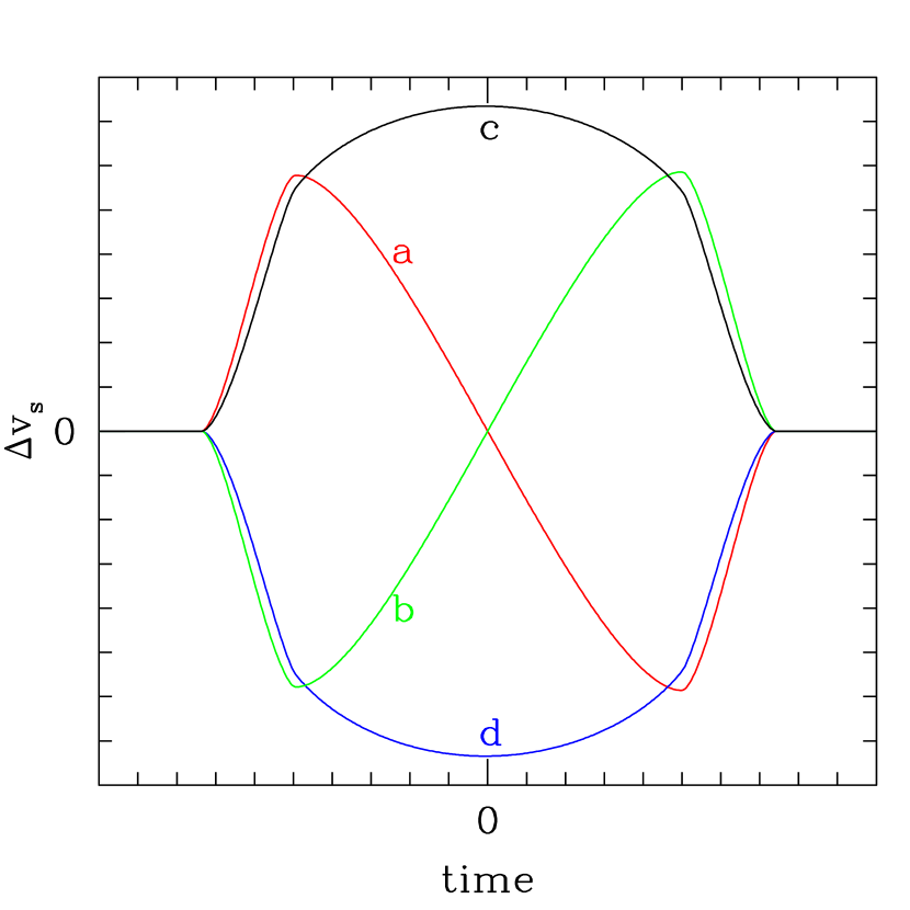
Figure 4: Schematic illustration of the velocity curve anomaly due to the RM effect. The four different paths of a planet, a-d, in the left panel correspond to the velocity curves in the right panel.

Equation (37) is the basic relation between $I(x,z)$ and $\Delta v_{s}$ in our subsequent analysis. Figure 4 shows a schematic illustration of the RM effect. Depending on the inclination and the orbital rotation direction relative to the stellar spin axis, the velocity curve anomaly due to the RM effect exhibits rather different behavior.

The remaining task is to evaluate the integrals adopting a certain model of a stellar surface intensity $I(x,z)$. Note that previous literature in the analytic study of radial velocity curves focused on expressing the integrals in the radial velocity shift (37) in terms of Kopal’s associated $\alpha$-functions under some model assumptions of the stellar intensity (e.g., Hosokawa, 1953; Kopal, 1990). While such detailed and exact approaches are required for stellar eclipsing binaries, the evaluation of the $\alpha$-function is a demanding numerical task. Furthermore, for those systems a variety of effects become important, including limb darkening, distortion of stars due to their rotation and tidal interaction, the reflection effect (heating by the radiant energy of the companion), and gravity darkening (variation of the surface brightness due to the local surface gravity acceleration change). For the extrasolar planetary systems, on the other hand, the radius and mass of a planet are significantly smaller than those of the host star. Thus, most of those effects can be safely neglected, and one can derive simpler, and still practically useful, analytic formulae applying perturbative expansion. In what follows, we present such analytic expressions for the RM effect with and without the stellar limb darkening.

4 Analytic expressions for a uniform stellar disk (without limb darkening)

As a step toward an analytic model for the RM effect for extrasolar planetary systems, let us consider first an idealistic case in which the limb-darkening effect is neglected. We also assume that the planet is completely optically thick and not rotating, which is also assumed in the next section. In this case, one can obtain the exact analytic expression even without the perturbative expansion. The intensity at $(x,z)$ on the uniform stellar surface becomes

$$I(x,z)=\cases{I_{0}&; $x^{2}+z^{2}\leq R_{s}^{2}$ and $(x-X_{p})^{2}+(z-Z_{p})^{2}\geq R_{p}^{2}$\cr\cr 0&; otherwise\cr},$$ (38)

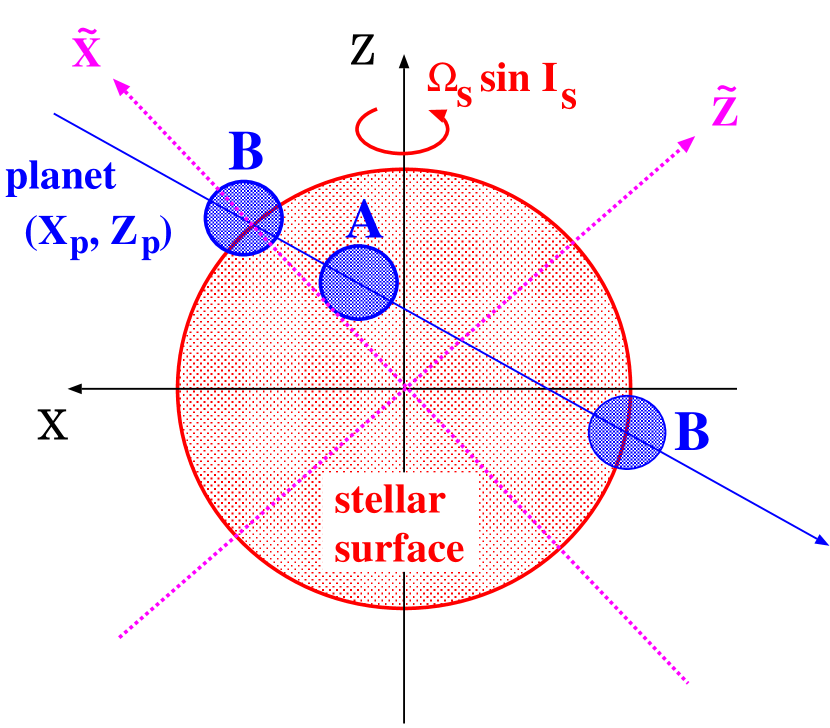
Figure 5: Planetary transit: ingress, complete transit, and egress phases.

where ${\mbox{\boldmath${X}$}}_{p}=(X_{p},Y_{p},Z_{p})$ is the position of the center of the planet and $R_{s}$ and $R_{p}$ denote the radii of the star and the planet, respectively. We evaluate equation (37) at complete transit, ingress, and egress phases in the following subsections (see Fig.5).

4.1 Complete transit phase

During a complete transit phase, the position of the planet satisfies the relation $\left(X_{p}^{2}+Z_{p}^{2}\right)^{1/2}<R_{s}-R_{p}$. Thus, the range of the integral in equation (37) is simply given by the stellar surface area with the entire planetary disk sutracted, i.e.,

$$\int\!\!\!\int dxdz\longrightarrow\int_{-R_{s}}^{R_{s}}dx\int_{-\sqrt{R_{s}^{2}-x^{2}}}^{\sqrt{R_{s}^{2}-x^{2}}}dz-\int_{X_{p}-R_{p}}^{X_{p}+R_{p}}dx\int_{Z_{p}-\sqrt{R_{p}^{2}-(x-X_{p})^{2}}}^{Z_{p}+\sqrt{R_{p}^{2}-(x-X_{p})^{2}}}dz.$$ (39)

Then we obtain

$$\int\!\!\!\int I(x,z)dxdz = \pi(R_{s}^{2}-R_{p}^{2})I_{0},$$ (40)

$$\int\!\!\!\int xI(x,z)dxdz = -X_{p}\pi R_{p}^{2}I_{0}.$$ (41)

Substituting these results into equation (37), we find

$$\Delta v_{s}=\Omega_{s}X_{p}\sin I_{s}\frac{\gamma^{2}}{1-\gamma^{2}}\qquad\left(\gamma\equiv\frac{R_{p}}{R_{s}}\right).$$ (42)

Equation (42) implies that the time dependence of the RM effect during the complete transit is entirely incorporated in the planet position, i.e., $X_{p}=X_{p}(t)$.

4.2 Ingress and egress phases

At ingress and egress phases, on the other hand, the location of the planet satisfies the relation, $R_{s}-R_{p}<\left(X_{p}^{2}+Z_{p}^{2}\right)^{1/2}<R_{s}+R_{p}$. Just for computational convenience, we rotate the coordinates in a time-dependent manner so that the planet is always located along the new $x$-axis:

$$\left(\begin{array}[]{c}\tilde{x}\\ \tilde{z}\end{array}\right)=\frac{1}{R_{s}\sqrt{X_{p}^{2}+Z_{p}^{2}}}\left(\begin{array}[]{cc}X_{p}&Z_{p}\\ -Z_{p}&X_{p}\end{array}\right)\left(\begin{array}[]{c}x\\ z\end{array}\right).$$ (49)

Then the position of the planet is given by

$$\left(\begin{array}[]{c}\tilde{X_{p}}\\ \tilde{Z_{p}}\end{array}\right)=\left(\begin{array}[]{c}1+\eta_{p}\\ 0\end{array}\right),$$ (54)

where

$$\eta_{p}=\frac{\sqrt{X_{p}^{2}+Z_{p}^{2}}}{R_{s}}-1.$$ (55)

In the new coordinates, equation (38) is rewritten as

$$I(\tilde{x},\tilde{z})=\cases{I_{0}&; $\tilde{x}^{2}+\tilde{z}^{2}\leq 1$ and $(\tilde{x}-1-\eta_{p})^{2}+\tilde{z}^{2}\geq\gamma^{2}$\cr\cr 0&; otherwise},$$ (56)

and the moments of the intensity reduce to

$$\int\!\!\!\int I(x,z)dxdz = R_{s}^{2}\left\{\pi I_{0}-\int\!\!\!\int_{S}I(\tilde{x},\tilde{z})d\tilde{z}d\tilde{x}\right\},$$ (57)

$$\int\!\!\!\int xI(x,z)dxdz = -\frac{R_{s}^{2}}{1+\eta_{p}}\int\!\!\!\int_{S}(X_{p}\tilde{x}-Z_{p}\tilde{z})I(\tilde{x},\tilde{z})d\tilde{z}d\tilde{x},$$ (58)

where the range of the integrals denoted by $S$ indicates the overlapping region between the stellar and the planetary disks and can be explicitly written as (dark shaded regions, Fig. 6):

$$\int\!\!\!\int_{S}d\tilde{z}d\tilde{x}~{}~{}~{}\longrightarrow~{}~{}~{}\int_{x_{0}}^{1}d\tilde{x}\int_{-\sqrt{1-\tilde{x}^{2}}}^{\sqrt{1-\tilde{x}^{2}}}d\tilde{z}\,\,+\,\,\int_{\tilde{X}_{p}-\gamma}^{x_{0}}d\tilde{x}\int_{-\sqrt{\gamma^{2}-(\tilde{x}-\tilde{X}_{p})^{2}}}^{\sqrt{\gamma^{2}-(\tilde{x}-\tilde{X}_{p})^{2}}}d\tilde{z}.$$ (59)

Note that the planetary and stellar circles intersect at $(x_{0},\pm z_{0})$, where

$$x_{0}=1-\frac{\gamma^{2}-\eta_{p}^{2}}{2(1+\eta_{p})},\quad~{}z_{0}=\sqrt{1-x_{0}^{2}}=\frac{\sqrt{(\gamma^{2}-\eta_{p}^{2})[(\eta_{p}+2)^{2}-\gamma^{2}]}}{2(1+\eta_{p})}.$$ (60)

Let us also introduce

$$\zeta\equiv 1+\eta_{p}-x_{0}=\frac{2\eta_{p}+\gamma^{2}+\eta_{p}^{2}}{2(1+\eta_{p})}.$$ (61)

Physically speaking, this corresponds to the separation between the intersection and the center of the planet along the $\tilde{X}$ axis, but we allow $\zeta$ to be negative (see Fig. 6) as well. Then equations (57) and (58) are analytically integrated as

$$\int\!\!\!\int_{S}I(\tilde{x},\tilde{z})d\tilde{z}d\tilde{x}=I_{0}\left[\,\,\sin^{-1}z_{0}-(1+\eta_{p})z_{0}+\gamma^{2}\cos^{-1}(\zeta/\gamma)\,\,\right],$$ (62)

and

$$\int\!\!\!\int_{S}(\tilde{x}X_{p}-\tilde{z}Z_{p})I(\tilde{x},\tilde{z})d\tilde{z}d\tilde{x}=I_{0}X_{p}(1+\eta_{p})\left[-z_{0}\zeta+\gamma^{2}\cos^{-1}(\zeta/\gamma)\right],$$ (63)

respectively.

Combining these results, we finally find that equation (37) reduces to

$$\Delta v_{\rm s}=\Omega_{s}X_{p}\sin I_{s}\,\,\frac{-z_{0}\zeta+\gamma^{2}\cos^{-1}(\zeta/\gamma)}{\pi-\sin^{-1}z_{0}+(1+\eta_{p})z_{0}-\gamma^{2}\cos^{-1}(\zeta/\gamma)}.$$ (64)

While the above expression for $\Delta v_{s}$ seems a bit complicated, this is the exact result for the radial velocity anomaly through relations (55), (60) and (61) in terms of the planet position $(X_{p},~{}Z_{p})$ specified by equation (18).

5 Effect of stellar limb darkening

To be more realistic, we now take account of the effect of limb darkening, which produces the radial dependence of the intensity of the stellar disk. Among the various models proposed so far (e.g., Claret, 2000), we adopt a linear limb-darkening law as the simplest, but a practically realistic one. Introducing the linear limb-darkening coefficient $\epsilon$, the stellar intensity is now given by

$$I(x,z)=\left\{\begin{array}[]{l}I_{0}\,\,\{1-\epsilon(1-\mu)\,\,\}~{}~{};~{}~{}x^{2}+z^{2}\leq R_{s}^{2}~{}~{}\mbox{and}~{}~{}(x-X_{p})^{2}+(z-Z_{p})^{2}\geq R_{p}^{2}\\ \\ 0~{}~{}~{}~{};~{}~{}\mbox{otherwise}\end{array}\right.,$$ (68)

where $\mu$ is the cosine of the angle between the line of sight and the vector normal to the local stellar surface :

$$\mu=\sqrt{1-\frac{x^{2}+z^{2}}{R_{s}^{2}}}.$$ (69)

With the limb-darkening effect, however, equation (37) can no longer be analytically integrated in an exact manner. Therefore, we construct approximate analytic formulae on the basis of the result without limb darkening ($\epsilon=0$; see section 4).

5.1 Complete transit phase

Applying the analytic results of §4.1 to the stellar intensity model (68), equation (37) is formally rewritten as

$$\Delta v_{\rm s}=\Omega_{s}X_{p}\sin I_{s}\,\,\frac{\gamma^{2}\,\{1-\epsilon(1-W_{2})\}}{1-\gamma^{2}-\epsilon\left\{\frac{1}{3}-\gamma^{2}(1-W_{1})\right\}},$$ (70)

where $W_{1}$ and $W_{2}$ are defined as

$$W_{1} = \frac{1}{\pi R_{p}^{2}}\,\int\!\!\!\int_{S}dxdz\sqrt{1-(x^{2}+z^{2})/R_{s}^{2}},$$ (71)

$$W_{2} = \frac{1}{X_{p}\,\pi R_{p}^{2}}\,\int\!\!\!\int_{S}dxdz\,\,x\sqrt{1-(x^{2}+z^{2})/R_{s}^{2}}.$$ (72)

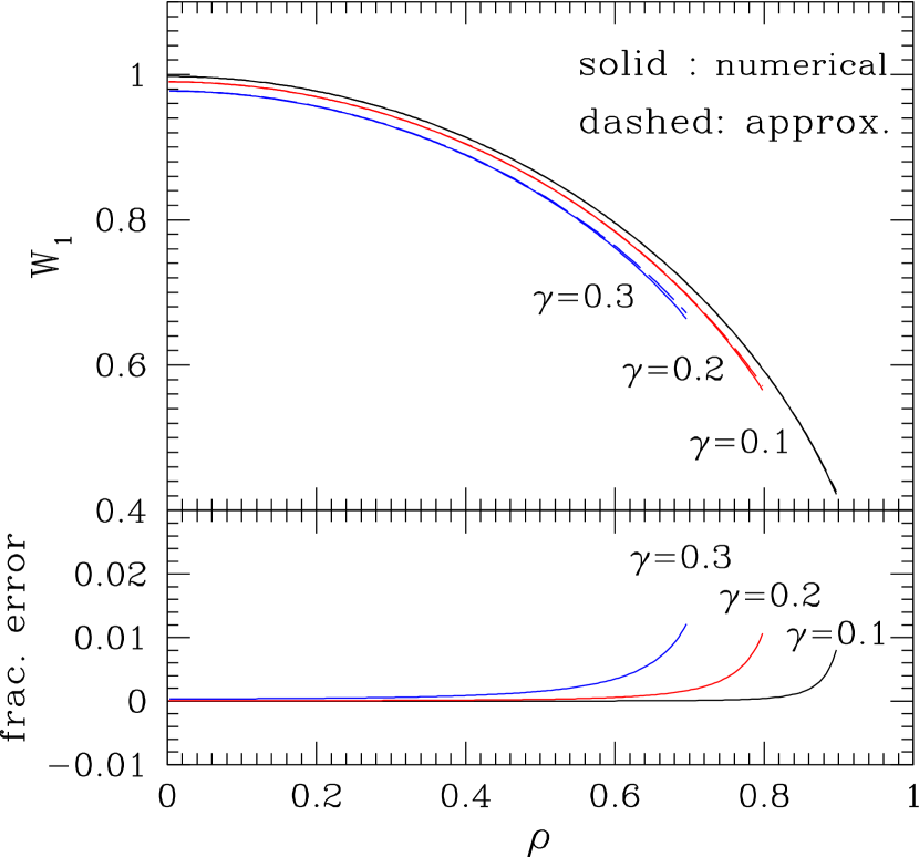
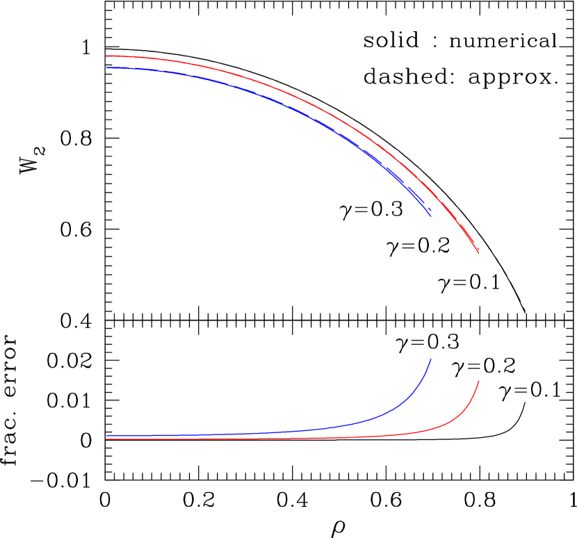
Figure 15: Top windows: Approximate vs. numerical evaluations of the integrals $W_{1}$ (left) and $W_{2}$ (right) as a function of $\rho=\left(X_{p}^{2}+Z_{p}^{2}\right)^{1/2}/R_{s}$. The solid lines represent the numerical evaluation of equations (A3) and (A16), while the dashed lines are the approximation based on the perturbative expansions (A15) and (A19). Note that the variable $\rho$ runs from $0$ to $1-\gamma$. Bottom windows: Fractional errors $W^{(\rm approx)}/W^{\rm(num)}-1$ for the integrals $W_{1}$ (left) and $W_{2}$ (right).

The above integrals are carried out over the entire planetary disk. As discussed in Appendix A.1, they reduce to one-dimensional integrals, which can be expanded with respect to $\gamma=R_{p}/R_{s}$. Specifically, equations (A15) and (A19) show perturbative expressions up to the fourth order in $\gamma$. The accuracy of the fourth-order perturbation expansion is within a few percent even for $\gamma\sim 0.3$ (Fig.15). In practice, however, the value of $\gamma$ is expected to be much smaller, $\gamma\lower 2.15277pt\hbox{$\;\buildrel<\over{\sim}\;$}0.1$. In this case, higher order terms in equations (A15) and (A19) contribute merely $\sim 1$% to equation (70), and one can safely use

$$W_{1}(\rho) \simeq 0,$$ (73)

$$W_{2}(\rho) \simeq (1-\rho^{2})^{1/2},$$ (74)

where $\rho\equiv\left(X_{p}^{2}+Z_{p}^{2}\right)^{1/2}/R_{s}$ ($0<\rho<1-\gamma$).

5.2 Ingress and egress phases

If the linear limb-darkening effect is taken into account, equation (64), describing the ingress and egress phases, now becomes

$$\Delta v_{\rm s} = \Omega_{s}X_{p}\sin I_{s}$$ (76)

$$\times\,\,\frac{\displaystyle(1-\epsilon)\left\{-z_{0}\zeta+\gamma^{2}\cos^{-1}(\zeta/\gamma)\right\}+\frac{\epsilon}{1+\eta_{p}}\,\,W_{4}}{\pi\left(1-\frac{1}{3}\epsilon\right)-(1-\epsilon)\left\{\sin^{-1}z_{0}-(1+\eta_{p})z_{0}+\gamma^{2}\cos^{-1}(\zeta/\gamma)\right\}-\epsilon\,\,W_{3}},$$

where $W_{3}$ and $W_{4}$ are defined by

$$W_{3} = \int\!\!\!\int_{S}d\tilde{x}d\tilde{z}\sqrt{1-\tilde{x}^{2}-\tilde{z}^{2}},$$ (77)

$$W_{4} = \int\!\!\!\int_{S}d\tilde{x}d\tilde{z}\,\,\tilde{x}\sqrt{1-\tilde{x}^{2}-\tilde{z}^{2}}.$$ (78)

Appendix A.2 derives approximate analytic expressions (A29) and (A30) for equations (77) and (78), respectively, assuming that $\gamma\ll 1$. Again, if $\gamma\lower 2.15277pt\hbox{$\;\buildrel<\over{\sim}\;$}0.1$, they can be safely set as

$$W_{3} \simeq 0,$$ (79)

$$W_{4} \simeq \frac{\pi}{2}\,\,\gamma(\gamma-\zeta)\,\,x_{c}\,\,\frac{g(x_{c}\,;\,\eta_{p},\,\gamma)}{g(1-\gamma;\,-\gamma,\,\gamma)}\,\,W_{2}(1-\gamma),$$ (80)

where

$$x_{c} = x_{0}+\frac{\zeta-\gamma}{2},$$ (81)

$$g(x;\,\eta_{p},\,\gamma) = (1-x^{2})\sin^{-1}\left\{\frac{\gamma^{2}-(x-1-\eta_{p})^{2}}{1-x^{2}}\right\}^{1/2}$$ (83)

$$~{}~{}~{}~{}~{}~{}+\sqrt{\{\gamma^{2}-(x-1-\eta_{p})^{2}\}\{1-x^{2}-\gamma^{2}+(x-1-\eta_{p})^{2}\}}.$$

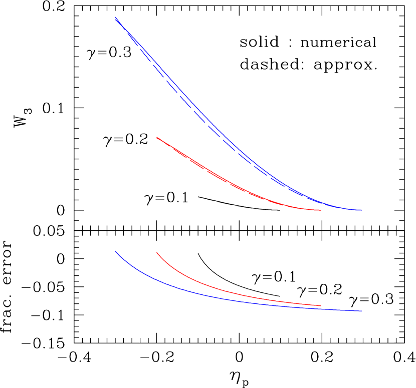
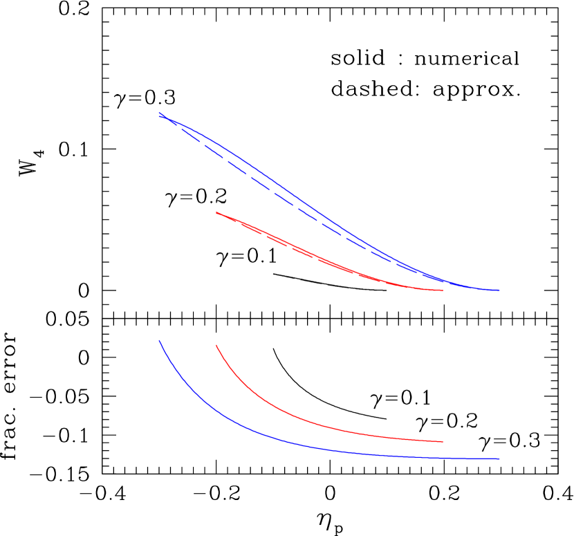
Figure 16: Top windows: Approximate vs. numerical evaluations of the integrals $W_{3}$ (left) and $W_{4}$ (right) as a function of $\eta_{p}$. The solid lines represent the numerical evaluation of equations (A20) and (A21), while the dashed lines are the approximation based on the perturbative expansions (A29) and (A30). Note that the variable $\eta_{p}$ runs from $-\gamma$ to $+\gamma$. Bottom windows: fractional errors $W^{\rm(approx)}/W^{\rm(num)}-1$ for the integrals $W_{3}$ (left) and $W_{4}$ (right).

As shown in Figure 16, the accuracy of equations (79) and (80) is typically within a fractional error of $5\%$-$10\%$ percent. Nevertheless, their contribution to the total error budget for the velocity anomaly (76) is within a few percent (see §6.2). Thus, equations (79) and (80) are practically good approximations in most cases.

6 Application to the HD 209458 system

So far, HD 209458 is the only extrasolar planetary system in which the RM effect is detected; Queloz et al. (2000) reported the first detection of this effect with ELODIE spectrograph on the 193 cm telescope of the Observatoire de Haute Provence. They numerically computed the radial velocity anomaly due to the RM effect for a variety of model parameters and compared these with the observed radial curves. They concluded that $\alpha=\pm 3.\!\!^{\circ}9{+18^{\circ}\atop-21^{\circ}}$ and $V\sin I_{s}=3.75\pm 1.25$ km s^-1, where $\alpha$ is the angle between the planet’s orbital plane and the star’s apparent equatorial plane and $V$ denotes the stellar surface velocity. These are written as $\alpha=\cos^{-1}(\sin i\cos\lambda)$ and $V=R_{s}\Omega_{s}$ according to the notation of our current paper. We summarize the current estimates of the stellar and planetary parameters for HD 209458 in Table 2 and the best solution for the spin parameters by Queloz et al. (2000) in Table 3. Since HD 209458 remains the best target for the precise measurement of the RM effect, we consider in this section the extent to which one can improve the constraints on the spin parameters with our analytic formulae.

6.1 Parameter dependence

Adopting the linear limb-darkening law for the stellar intensity model, the RM effect for a system in the Keplerian orbit is specified by $10$ parameters: the limb-darkening coefficient $\epsilon$, the orbital parameters of the system ($a$, $e$, $i$, $\varpi$, and $P_{\rm orb}$), the size of the stellar and planetary disks ($R_{s}$ and $R_{p}$), the projected stellar surface velocity $V\sin I_{s}$, and the projected angle between the stellar spin axis and the normal direction of the orbital plane $\lambda$. Except for the last two parameters ($V\sin I_{s}$ and $\lambda$), these can be independently determined from the usual radial velocity and transiting photometric data, at least in principle. This is indeed the case for the HD 209458 system (see Table 2). Therefore, it is natural to ask about the extent to which one can put constraints on the two parameters $V\sin I_{s}$ and $\lambda$ from the radial velocity anomaly during the transit due to the RM effect.

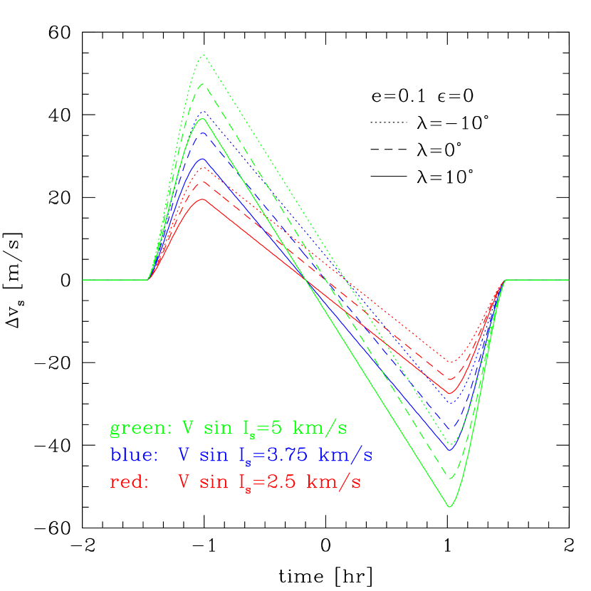
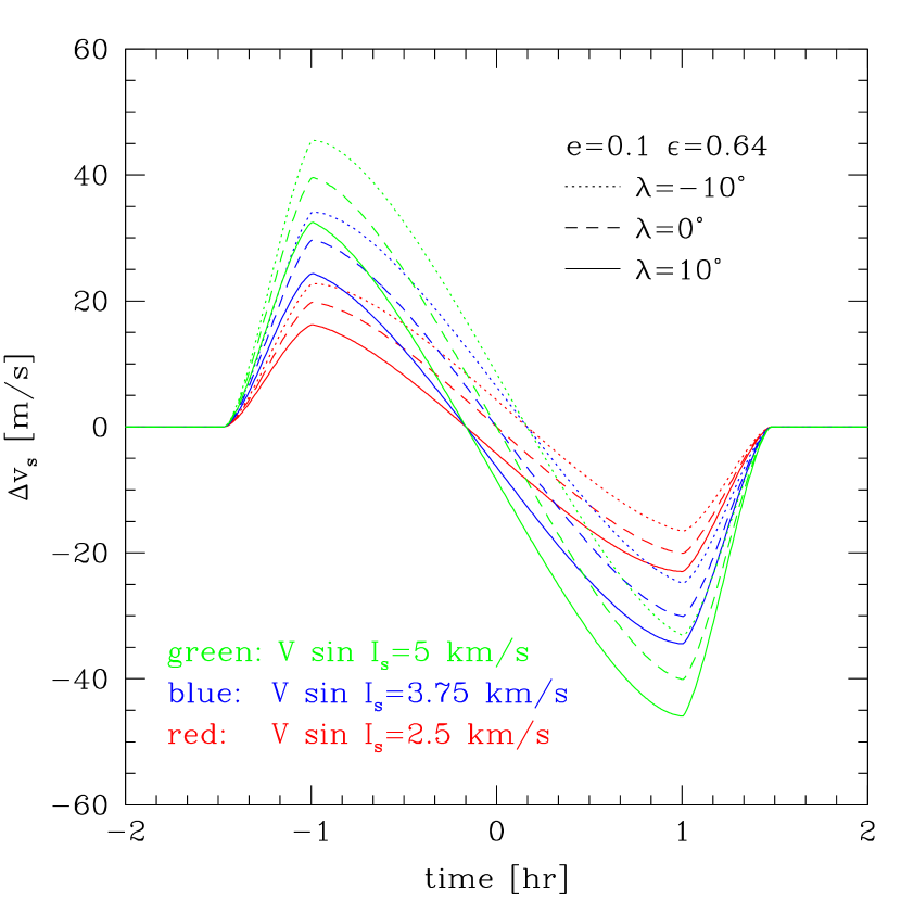
Figure 7: Analytic radial velocity curves for the RM effect without stellar limb darkening ($\epsilon=0$).

Figure 8: Same as Fig.8, but with a linear limb-darkening effect ($\epsilon=0.64$).

Consider first the sensitivity to the spin parameters ($V\sin I_{s}$, $\lambda$). Figures 8 and 8 illustrate our approximations for $\Delta v_{s}$ adopting the estimated parameters of the HD 209458 system (Table 2) with and without the stellar limb darkening (i.e., $\epsilon=0$ and $0.64$, specifically), respectively. The central transit epoch is chosen as $t=0$. Then ingress starts at $t=-1.55$ hr, the complete transit lasts for $-1.07<t<1.08$ hr, and egress ends at $t=1.56$ hr for $e=0.1$ (sometimes these four epochs are referred to as the first, second, third, and fourth contacts, respectively). The range of the spin parameters, $V\sin I_{s}$ and $\lambda$, adopted in these figures roughly covers the uncertainties of the values of Queloz et al. (2000).

Comparison of the two figures indicates that the radial velocity anomaly $\Delta v_{s}$ is also sensitive to the linear limb-darkening coefficient $\epsilon$. Obviously the amplitude of the radial velocity shift $\Delta v_{r}$ is sensitive to $V\sin I_{s}$. The projected angle $\lambda$ shifts the zero point of the radial velocity anomaly at earlier ($\lambda>0$) and later ($\lambda<0$) epochs for the orbital inclination $i<90^{\circ}$. This produces an asymmetry of the shape of the radial velocity anomaly. Note that the behavior becomes opposite for the inclination $i>90^{\circ}$, corresponding to the parameter degeneracy between $(i,\lambda)$ and $(180^{\circ}-i,-\lambda)$. Because of the different dependence of the overall radial velocity anomaly on the spin parameters $(V\sin I_{s},~{}\lambda)$, one can put more stringent constraints on those if our formulae are combined with future precision data attainable by 8 – 10 m class telescopes with a high dispersion spectrograph (HDS) such as Subaru HDS.

Before addressing this issue in detail, it is helpful to clarify the dependence of the RM effect on the other remaining parameters. To investigate this, we quantify the variation of the radial velocity shift with respect to a specific parameter change $p\sim p+dp$ by

$$\delta\Delta v_{s}\equiv\lim_{dp\to 0}\frac{\Delta v_{s}(p+dp)-\Delta v_{s}(p)}{dp/p}$$ (84)

for $p=a,R_{s},R_{p},P_{\rm orb},V\sin I_{s},\epsilon,$ and $e$. In practice, we systematically decrease the value of $dp/p$ for each parameter down to $10^{-6}$ and ensure the convergence of the derivative. For the angular parameters $p=i,\varpi,$ and $\lambda$, we simply take their scaling values at $10^{\circ}$:

$$\delta\Delta v_{s}\equiv\lim_{dp\to 0}\frac{\Delta v_{s}(p+dp)-\Delta v_{s}(p)}{dp/10^{\circ}}.$$ (85)

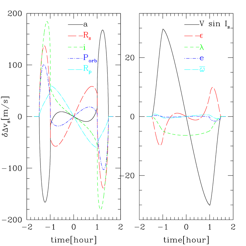
Figure 9: Variation of radial velocity shift with respect to a parameter variation $p\to p+dp$ as a function of time. The vertical axis denotes the variation of radial velocity shift normalized by the fractional error in each parameter $dp/p$ ( eqs. [84] and [85] for left and right panels, respectively). These quantities are evaluated around the fiducial values for the HD 209458 system summarized in Table 2 using the analytic formulae for the RM effect.

Here, we confirm the convergence of the derivative by decreasing the value of $dp/10^{\circ}$ down to $10^{-6}$ in these cases. Our analytic formulae are indeed useful in evaluating these quantities at the fiducial parameters of the HD 209458 system (Tables 2 and 3). The results are plotted in Figure 9 as a function of time. Note that our definition of $\delta\Delta v_{s}$ is normalized by the fractional error in the parameter, i.e., $dp/p$.

Figure 9 clearly shows that the stellar radius $R_{s}$ and the orbital parameters $a$, $i$, and $P_{\rm orb}$ sensitively change the normalized radial velocity variation $\delta\Delta v_{s}$ at the ingress and egress phases, while the spin parameters $(V\sin I_{s},\lambda)$ have a relatively smaller effect on $\delta\Delta v_{s}$. To quantify the actual deviation of the radial velocity shift caused by the systematic errors in the observation, we must multiply the observational uncertainty listed in Table 2. Then it turns out that the most sensitive parameter is $V\sin I_{s}$, causing the $12$m s^-1 variation of the radial velocity shift. The other parameters change the radial velocity shift at the ingress and egress phases by less than $5$m s^-1. This amplitude itself is comparable to the $\delta\Delta v_{s}$ induced by the uncertainty of the projected angle $\lambda$. Nevertheless, the different time-dependent effects of the various parameters can be used to break the parameter degeneracy, which would enable an accurate determination of the spin parameters $\lambda$ and $V\sin I_{s}$. In addition, Figure 9 even suggests that a more precise determination of the orbital parameters other than the spin parameters is also possible by combining the RM effect with the usual radial velocity measurement.

6.2 Accuracy of our formulae

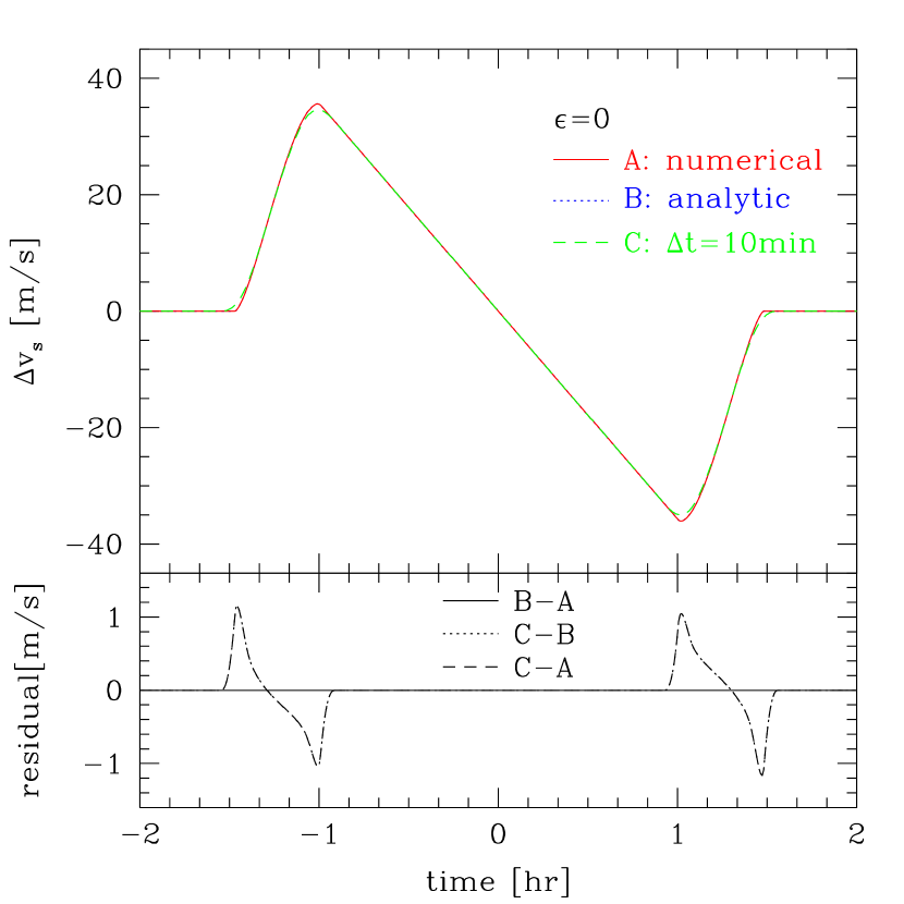
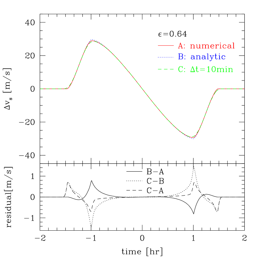
Figure 10: Comparison of different models of the radial velocity anomaly curves for the HD 209458 system without limb darkening ($\epsilon=0$). The top panel shows the radial velocity shifts obtained from the numerical evaluation of expression (37) (solid curve) and the analytic formulae with and without the effect of exposure time (dotted and dashed curves, respectively). The bottom panel shows the residuals between the two radial velocity shifts among three curves.

Figure 11: Same as Fig.11, but with limb darkening ($\epsilon=0.64$).

While our analytic formulae presented in the previous section will improve the efficiency of the parameter estimations relative to fully numerical approaches, we have to address a couple of issues before applying them to real data: their accuracy and the effect of the finite exposure time. Our formulae with limb darkening are derived on the basis of an empirical approximation to the integrals of the stellar surface intensity (§5). Furthermore, the real data do not instantaneously sample the radial velocity, but are averaged over a finite exposure time. We directly test those effects against the numerical solutions of equation (37). Figures 11 and 11 compare three results: numerical integration of equation (37), our analytic formulae, and the numerical average of equation (37) over a $\Delta t=10$ minute exposure time (in practice, we separately average the denominator and the numerator of the analytic formulae assuming $\Delta t=10$ minutes and then take their ratio). These results are labeled A, B, and C and plotted in solid, dotted, and dashed curves, respectively, in the top panels.

For $\epsilon=0$, the analytic formulae (curve B) are exact, and the completely negligible difference A$-$B should be regarded as a welcome check of the accuracy of our numerical integration scheme. The bottom panels suggest that the three results agree within an accuracy of $\sim 1$m s^-1, which is below the typical radial velocity sensitivity achieved ($\sim 3$m s^-1) and is only comparable to the latest achievement by HARPS (Santos et al., 2004). Therefore, as far as the HD 209458 system is concerned, we can safely use our analytic formulae as useful templates for the RM effect even if a finite exposure time of the order of 10 minutes is taken into account.

6.3 Mock analysis of the spin parameter estimation

Now we are in a position to ask whether our formulae combined with precision spectroscopic data can improve the previous constraints on the spin parameters $(\Omega_{s}\sin I_{s},\,\lambda)$, among others. For this purpose, we create mock data for the radial velocity anomaly of the HD 209458 system and fit them to the analytic formulae. Basically, the mock data were created adopting the central values of the parameters listed in Tables 2 and 3, but assigned an overall Gaussian random error of the rms amplitude $5$ m s^-1, which is the level of precision achieved with the Subaru HDS assuming an exposure time of $\Delta t=10$ minutes (Winn et al., 2004). In light of the most recent sensitivity achieved by HARPS (Santos et al. 2004; $\sim 1$m s^-1), our error assignment may still be conservative if the error is not dominated by other possible systematic errors. To mimic the effect of the finite exposure time, we numerically integrate the denominator and the numerator of equation (37) separately over $\Delta t=10$ minutes. Then we take the ratio and assign the random error, as mentioned above.

Note that the number of independent data points during the transit phase ($\sim 3$ hr including the ingress and egress phases) is $16$ for $\Delta t=10$ minutes. The generated mock data are then fitted to the analytic radial velocity anomaly to estimate the spin parameters. Here, the fitting is performed assuming prior knowledge of the remaining eight parameters.

First, let us see how the spin parameters are reliably estimated from the $\chi^{2}$ fit. To examine this, we create $50,000$ mock realizations and calculate the joint probability distribution of the best-fit parameters under a certain prior knowledge of $R_{s}$, $R_{p}$, and $a$. We use the $\chi^{2}$ function,

$$\chi^{2}(V\sin I_{s},\lambda)=\sum_{i=1}^{N}\left\{\frac{\Delta v_{s,i}^{\rm data}-\Delta v_{s}^{\rm model}(V\sin I_{s},\lambda;t_{i})}{\sigma_{\scriptscriptstyle\Delta v}}\right\}^{2}$$ (86)

with $\sigma_{\scriptscriptstyle\Delta v}=5$m s^-1 and $N=16$. In this analysis, according to the result in Figure 9, we particularly focus on the five parameters $V\sin I_{s}$, $\lambda$, $R_{s}$, $R_{p}$, and $a$. Their input values are $3750$ m s^-1, $0^{\circ}$, $1.146{\rm R_{\odot}}$, $1.347{\rm R_{J}}$, and $0.0468$ AU, respectively. We assume a set of different prior values for $R_{s}$, $R_{p}$, and $a$ indicated in each panel of Figure 12 and then perform the $\chi^{2}$ minimization over $V\sin I_{s}$ and $\lambda$.

The results are plotted as contour levels in Figure 12. Here, the two contour curves in each panel represent the 1 and 2 $\sigma$ levels of the joint probability. The solid curves plotted along the horizontal and vertical axes are the probability distributions of $V\sin I_{s}$ and $\lambda$, respectively, each of which is the projection of the joint probability distribution over the other parameter. Note that in both cases the probability distribution is well approximated by a Gaussian distribution with 1 $\sigma$ values of $\sigma_{\scriptscriptstyle V\sin I_{s}}\simeq 310$ m s^-1 and $\sigma_{\lambda}\simeq 3.\!\!^{\circ}4$. This result indicates that the estimated value for $V\sin I_{s}$ is rather sensitive to the assumed value of the planetary radius $R_{p}$, while $\lambda$ can be estimated reliably even if $R_{p}$ is not known accurately. This comes from the fact that the velocity shift is roughly proportional to $V\sin I_{s}R_{p}^{2}$; however, the projected angle $\lambda$ is sensitive only to the asymmetry of the radial velocity shift curve. Another important aspect is that the uncertainty of the prior knowledge of the stellar radius has little effect on the parameter estimation.

The above analysis implies that with a suitably short exposure time, our formulae provide an unbiased estimation of the spin parameters statistically, if we have reasonably accurate prior knowledge of the other parameters of the system. In reality, however, it may be more relevant to ask about the reliability of the confidence level of the spin parameters derived from a single realization, rather than from the 50,000 realizations. This is related to the above analysis statistically, but perhaps it is more appropriate to the situation that one encounters in any observation. For this purpose, we randomly select one from the 50,000 realizations and compute 1 and 2 $\sigma$ confidence contours from the relative confidence levels,

$$\Delta\chi^{2}\equiv\chi^{2}(V\sin I_{s},\lambda)-\chi^{2}(V\sin I_{s,0},\lambda_{0}),$$ (87)

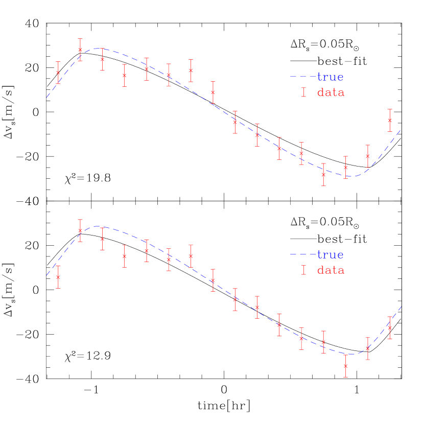
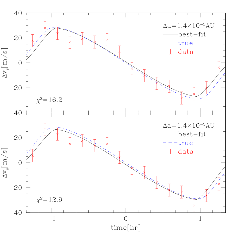
Figure 14: Comparison between the mock data for the radial velocity curves used in Fig.13 and the best-fit curves for the parameters $(V\sin I_{s},~{}\lambda)$ (solid curves) determined under the prior assumption of $(\epsilon,~{}e)$ for the fiducial parameters (top left), $\Delta R_{p}=0.06\,R_{\rm J}$ (top right), $\Delta R_{s}=0.05=\,R_{\odot}$ (bottom left), and $\Delta a=1.4\times 10^{-3}\,{\rm AU}$ (lower-right). The result depicted in the upper and lower window of each panel corresponds to the thin and thick contour lines in Fig.13, respectively. For comparison, we also plot the correct radial velocity curves in each plot (dashed curves).

where $V\sin I_{s,0}$ and $\lambda_{0}$ are the best-fit values. Figure 13 shows the estimated parameter regions on the $V\sin I_{s}$ versus $\lambda$ plane, and the best-fit values are indicated by the plus signs in each panel. The corresponding radial velocity curves are depicted in Figure 14, together with both the best-fit and the true curves (solid and dashed curves, respectively).

Basically, Figure 13 demonstrates that the spin parameters $V\sin I_{s}$ and $\lambda$ can be constrained around the best-fit values with the 1 $\sigma$ errors of $\Delta V\sin I_{s}\simeq\pm 300$m s^-1 and $\Delta\lambda\simeq\pm 4^{\circ}$, which greatly improves the uncertainties (by a factor of 4) relative to the previous result by Queloz et al. (2000, see Table 3).

7 Conclusions and discussion

We have discussed a methodology to estimate the stellar spin angular velocity and its direction angle with respect to the planetary orbit for transiting extrasolar planetary systems using the RM effect previously known in eclipsing binary stars (Rossiter, 1924; McLaughlin, 1924; Kopal, 1990). In particular we have derived analytic expressions of the radial velocity anomaly, $\Delta v_{s}$, which are sufficiently accurate for extrasolar planetary systems. If the stellar limb darkening is neglected, the expression is exact. We have extended the result to the case with limb darkening and obtained approximate but accurate analytic formulae. For a typical value of $\gamma=R_{p}/R_{s}\sim 0.1$, the formulae reduce to a simple form (eqs.[70], [73], [74], [76], [79], and [80]):

$$\Delta v_{\rm s}=\Omega_{s}X_{p}\sin I_{s}\,\,\frac{\gamma^{2}\,\{1-\epsilon(1-W_{2})\}}{1-\gamma^{2}-\epsilon\left\{\frac{1}{3}-\gamma^{2}\right\}}$$ (88)

during the complete transit phase and

$$\Delta v_{\rm s} = \Omega_{s}X_{p}\sin I_{s}\,\,\frac{\displaystyle(1-\epsilon)\left\{-z_{0}\zeta+\gamma^{2}\cos^{-1}(\zeta/\gamma)\right\}+\frac{\epsilon}{1+\eta_{p}}\,\,W_{4}}{\pi\left(1-\frac{1}{3}\epsilon\right)-(1-\epsilon)\left\{\sin^{-1}z_{0}-(1+\eta_{p})z_{0}+\gamma^{2}\cos^{-1}(\zeta/\gamma)\right\}}$$ (89)

during the egress/ingress phases, where

$$W_{2} = \frac{(R_{s}^{2}-X_{p}^{2}-Z_{p}^{2})^{1/2}}{R_{s}},$$ (90)

$$W_{4} = \frac{\pi}{2}\,\,\gamma^{3/2}(2-\gamma)^{1/2}(\gamma-\zeta)\,\,x_{c}\,\,\frac{g(x_{c}\,;\,\eta_{p},\,\gamma)}{g(1-\gamma;\,-\gamma,\,\gamma)},$$ (91)

where $g(x;a,b)$ is defined in equation (A23). The definition and the meaning of the variables in the above expressions are summarized in Table 1.

The numerical accuracy of the above formulae was checked using a specific example of the transiting extrasolar planetary system, HD 209458, and we found that they are accurate within a few percent. Our analytic formulae for the radial velocity anomaly are useful in several ways. One can estimate the planetary parameters much more efficiently and easily, since one does not have to resort to computationally demanding numerical modeling. Furthermore, the resulting uncertainties of the fitted parameters and their correlations are easily evaluated. To illustrate these advantages specifically, we performed a parameter estimation applying the formulae against mock data for HD 209458. We showed that with precision data obtainable by 8–10 m class telescopes such as Subaru HDS, our formulae improve the efficiency and robustness of estimating the spin parameters, $V\sin I_{s}$ and $\lambda$. Furthermore, the combined data analysis with asteroseismology (e.g., Gizon & Solanki, 2003) and/or the correlation between the mean level of emission and the rotation period (e.g., Noyes et al., 1985) may break the degeneracy between $V$ and $I_{s}$ in extrasolar planetary systems.

Among the recently discovered transiting extrasolar planetary systems, i.e., TrES-1 by the Trans-Atlantic Exoplanet Survey (Alonso et al., 2004) and OGLE-TR 10, 56, 111, 113, 132 by the Optically Gravitational Lens Event survey (e.g., Udalski et al., 2002a, b, c, 2003; Konacki et al., 2003; Bouchy et al., 2004; Pont et al., 2004), TrES-1 has similar orbital period and mass to those of HD 209458b, but its radius is smaller. Thus, it is an interesting target to determine the spin parameters via the RM effect; if its planetary orbit and the stellar rotation share the same direction as discovered for the HD 209458 system, it would be an important confirmation of the current view of planet formation out of the protoplanetary disk surrounding the protostar. If not, the result would be more exciting and even challenge the standard view, depending on the value of the misalignment angle $\lambda$.

We also note that the future satellites Corot and Kepler will detect numerous transiting planetary systems, most of which will be important targets for the RM effect in 8 - 10 m class ground-based telescopes. We hope that our analytic formulae presented here will be a useful template in estimating parameters for those stellar and planetary systems.

Finally, it is interesting to note that the RM effect may even be used as yet another new detection method of transiting planetary systems. For the HD 209458 system, the stellar radial velocity amplitude due to the Kepler motion is around 100 m s^-1. Since the stellar rotation velocity is around 4 km s^-1, the maximum radial velocity anomaly due to the RM effect is $\sim 40(\gamma/0.1)^{2}$m s^-1 and thus is very close to the former. On the other hand, the latter could be significantly larger if the host star rotates faster, and/or the host star (the planet) has a smaller (larger) radius. In extreme cases, the radial velocity curve, with a periodicity of a few days for instance, is barely detectable, but the velocity anomaly is quite visible for a few hours of the transiting phase. Thus, the conventional radial velocity curve analysis might have missed some of the potentially interesting spectroscopic signature of transiting planets. A search for such specific signatures deserves an attempt against existing or future spectroscopic samples that do not show any clear conventional feature of radial velocity periodicity.

In conclusion, we have demonstrated that the radial velocity anomaly due to the RM effect provides a reliable estimation of spin parameters. Combining data with the analytic formulae for radial velocity shift $\Delta v_{s}$, this methodology becomes a powerful tool in extracting information on the formation and the evolution of extrasolar planetary systems, especially the origin of their angular momentum. Although it is unlikely, we may even speculate that a future RM observation may discover an extrasolar planetary system in which the stellar spin and the planetary orbital axes are antiparallel or orthogonal. This would have a great impact on the planetary formation scenario, which would have to invoke an additional effect from possible other planets in the system during the migration or the capture of a free-floating planet. While it is premature to discuss such extreme possibilities at this point, the observational exploration of transiting systems using the RM effect is one of the most important probes for a better understanding of the origin of extrasolar planets.

Appendix A Approximation of integrals

In this appendix, the approximate expressions for the integrals $W_{i}~{}(i=1\sim 4)$ defined in section 5 are derived. Below, we present the results separately for the integrals $W_{1}$ and $W_{2}$ in Appendix A.1 and for $W_{3}$ and $W_{4}$ in Appendix A.2.

A.1 Integrals $W_{1}$ and $W_{2}$

First, consider the integral $W_{1}$. For further reduction of the integral, it is convenient to rewrite equation (71) in terms of the new variables

$$(x,z)=R_{p}\,\sigma(\cos\varphi,\sin\varphi)+(X_{p},Z_{p}),~{}~{}~{}~{}~{}(X_{p},Z_{p})=R_{s}\rho(\cos\theta,\sin\theta).$$ (A1)

Then we obtain

$$W_{1} = \frac{1}{\pi}\int_{0}^{1}d\sigma\int_{0}^{2\pi}d\varphi\,\,\sigma\sqrt{1-\rho^{2}\sin^{2}{(\theta-\varphi)}-\{\gamma\sigma+\rho\cos{(\theta-\varphi)}\}^{2}}.$$ (A2)

Here, the variable $\rho$ runs from $0$ to $1-\gamma$. In the above expression, the integral over $\sigma$ is analytically expressed, and a part of it is further integrated out. The resulting expression becomes

$$W_{1} = \frac{2}{3\gamma^{2}}\,(1-\rho^{2})^{1/2}\,\left(1-\frac{1}{4}\rho^{2}\right)\,-\,w_{A}\,+\,w_{B},$$ (A3)

where $w_{A}$ and $w_{B}$ are given by

$$w_{A} = \frac{1}{\pi\,\gamma^{2}}\,\,\left[\frac{1}{3}\int_{0}^{2\pi}d\varphi(1-\rho^{2}-\gamma^{2}-2\rho\gamma\ \cos{\varphi})^{3/2}\right.$$ (A5)

$$\left.~{}~{}~{}~{}~{}~{}~{}~{}~{}~{}~{}~{}~{}+\frac{1}{2}\int_{0}^{2\pi}d\varphi\,\,(\rho^{2}\cos\varphi+\rho\gamma)\cos\varphi(1-\rho^{2}-\gamma^{2}-2\rho\gamma\cos\varphi)^{1/2}\right],$$

$$w_{B} = \frac{1}{2\pi\gamma^{2}}\int_{0}^{2\pi}d\varphi\,\,\rho\cos\varphi(1-\rho^{2}\sin^{2}\varphi)$$ (A7)

$$~{}~{}~{}~{}~{}~{}~{}~{}~{}~{}~{}~{}~{}~{}~{}~{}~{}~{}\times\,\left\{\sin^{-1}\left(\frac{\rho\cos\varphi}{\sqrt{1-\rho^{2}\sin^{2}\varphi}}\right)-\sin^{-1}\left(\frac{\gamma+\rho\cos\varphi}{\sqrt{1-\rho^{2}\sin^{2}\varphi}}\right)\right\}.$$

Note that the integrals $w_{A}$ and $w_{B}$ are analytically expressed in terms of the complete elliptic integrals of the first kind $K(m)$, the second kind $E(m)$, and the third kind $\Pi(n,m)$:

$$w_{A} = \frac{1}{45\pi\gamma^{4}}\{1-(\gamma+\rho)^{2}\}^{1/2}$$ (A10)

$$\times\,\,\,\left[\left\{3(1-\rho^{2})^{2}-\gamma^{2}(71-17\rho^{2})+68\gamma^{4}\right\}\,E(m)\right.$$

$$~{}~{}~{}~{}~{}~{}~{}~{}~{}~{}~{}\left.-\{(\gamma-\rho)^{2}-1\}(3\rho^{2}-3+8\gamma^{2})\,K(m)\right],$$

$$w_{B} = \frac{2}{3\gamma^{2}}\left[1-(1-\rho^{2})^{1/2}\left(1-\frac{\rho^{2}}{4}\right)\right]$$ (A11)

$$+\frac{1}{45\pi\gamma^{4}[1-(\gamma+\rho)^{2}]^{1/2}}$$

$$~{}~{}\times\left\{\left[2\gamma^{6}+(29-7\rho^{2})\gamma^{4}+(26-34\rho^{2}+8\rho^{4})\gamma^{2}+3(1-\rho^{2})^{3}\right]K(m)\right.$$

$$~{}~{}~{}~{}~{}~{}\left.+\left[1-(\rho+\gamma)^{2}\right]\left[2\gamma^{4}+(31-7\rho^{2})\gamma^{2}-3(1-\rho^{2})^{2}\right]E(m)\right\}$$

$$-\frac{2}{3\pi\gamma^{2}[1-(\gamma+\rho)^{2}]^{1/2}}\left\{\left[1-n(\rho+\gamma)/2\rho\right]\Pi(n,m)+\rm{c.c.}\right\},$$

where c.c. denotes the complex conjugate, $n=2\rho\left[\rho-i(1-\rho^{2})^{1/2}\right]$, and $m=-4\gamma\rho/[1-(\gamma+\rho)^{2}]$. To evaluate equations (A10) and (A11), careful treatments are required at the edge $\rho=1-\gamma$, where the argument of the elliptic integral and coefficients of $K(m)$ and $\Pi(n,m)$ in $w_{B}$ apparently diverge. Since we are concerned with planetary systems with a small ratio $R_{p}\ll R_{s}$, it is practically useful to derive the approximate expressions. In this case, we do not have to use the complicated expressions (A10) and (A11), but can expand the integrands (A2) and/or (A5), (A7) in powers of $\gamma=R_{p}/R_{s}$. Then each term in the expansion with respect to $\gamma$ can be analytically integrated. The results up to the second order in $\gamma$ become

$$w_{A} \simeq \frac{2}{3\gamma^{2}}\,\,(1-\rho^{2})^{1/2}\left(1-\frac{1}{4}\rho^{2}\right)\,\,-\,\,\frac{1}{16}\,\,\frac{15\rho^{4}-28\rho^{2}+16}{(1-\rho^{2})^{3/2}}$$ (A13)

$$~{}~{}~{}~{}~{}~{}~{}~{}~{}~{}~{}~{}~{}~{}~{}~{}~{}~{}~{}-\,\gamma^{2}\,\,\frac{1}{128}\,\,\frac{17\rho^{6}-64\rho^{4}+104\rho^{2}-32}{(1-\rho^{2})^{7/2}}\,\,+\,\,{\cal O}(\gamma^{4}),$$

$$w_{B} \simeq -\frac{1}{4}\,\,\frac{\rho^{2}(1-\rho^{2}/4)}{(1-\rho^{2})^{3/2}}\,\,-\,\,\gamma^{2}\,\,\frac{1}{128}\,\,\frac{\rho^{2}(24+\rho^{4})}{(1-\rho^{2})^{7/2}}\,\,+\,\,{\cal O}(\gamma^{4}).$$ (A14)

Substituting these expressions into equation (A3) and collecting the terms in powers of $\gamma$, we finally obtain

$$W_{1}\simeq(1-\rho^{2})^{1/2}\,\,-\,\,\gamma^{2}\,\frac{2-\rho^{2}}{8(1-\rho^{2})^{3/2}}+{\cal O}(\gamma^{4}).$$ (A15)

Next, consider the integral $W_{2}$, whose analytic expression is also obtained through the same procedure as mentioned above. Using equations (A1), one writes equation (72) as

$$W_{2}=W_{1}+w_{C},$$ (A16)

where $w_{C}$ is given by

$$w_{C}=\frac{\gamma}{\pi\,\rho\cos\theta}\,\,\int_{0}^{1}d\sigma\int_{0}^{2\pi}d\varphi\,\,\sigma^{2}\cos\varphi\sqrt{1-\rho^{2}\sin^{2}{(\theta-\varphi)}-\{\gamma\sigma+\rho\cos{(\theta-\varphi)}\}^{2}}.$$ (A17)

In the above expression, the integral over $\sigma$ is analytically performed, and the resulting expression for the integrand is expanded in powers of $\gamma$. Further integrating it over $\varphi$, we obtain

$$w_{C}\simeq-\gamma^{2}\,\,\frac{1}{4(1-\rho^{2})^{1/2}}+{\cal O}(\gamma^{4}).$$ (A18)

Thus, the perturbative expansion for $W_{2}$ becomes

$$W_{2}\simeq(1-\rho^{2})^{1/2}\,\,-\,\,\gamma^{2}\,\frac{4-3\rho^{2}}{8(1-\rho^{2})^{3/2}}+{\cal O}(\gamma^{4}).$$ (A19)

In Figure 15, to check the validity of the perturbation results, the approximate expressions for the integrals $W_{1}$ and $W_{2}$ are plotted as a function of $\rho$. The results are then compared with those obtained from the numerical integration. As is expected, the perturbative expressions (A15) and (A19) give a quite accurate approximation as long as the ratio of the planetary radius to the stellar radius is small. Note that the approximation is even better for the slightly larger value $\gamma=0.3$, with a few percent level for the fractional error.

A.2 Integrals $W_{3}$ and $W_{4}$

As for the integrals $W_{3}$ and $W_{4}$ given by equations (77) and (78), one can partially evaluate the integrals with the knowledge of the integral region (59). The resulting forms are summarized as

$$W_{3} = \frac{\pi}{6}(1-x_{0})^{2}(2+x_{0})+\int_{x_{0}+\zeta-\gamma}^{x_{0}}d\tilde{x}\,\,g(\tilde{x};\,\eta_{p},\,\gamma),$$ (A20)

$$W_{4} = \frac{\pi}{8}(1-x_{0}^{2})^{2}+\int_{x_{0}+\zeta-\gamma}^{x_{0}}d\tilde{x}\,\,\tilde{x}\,\,g(\tilde{x};\,\eta_{p},\,\gamma),$$ (A21)

where we defined the function $g(\tilde{x};\,\eta_{p},\,\gamma)$ as

$$g(\tilde{x};\,\eta_{p},\,\gamma) \equiv (1-\tilde{x}^{2})\sin^{-1}\left\{\frac{\gamma^{2}-(\tilde{x}-1-\eta_{p})^{2}}{1-\tilde{x}^{2}}\right\}^{1/2}$$ (A23)

$$~{}+\sqrt{2(1+\eta_{p})(x_{0}-x)\{\gamma^{2}-(\tilde{x}-1-\eta_{p})^{2}\}}.$$

Since the above one-dimensional integrals cannot be evaluated analytically, one may derive an approximate expression applicable to the $\gamma\ll 1$ cases. Note, however, that a naive treatment by the perturbative expansion regarding $\gamma$ as a small parameter can break down at $\eta_{p}\simeq-\gamma$. Even in the $\eta_{p}>\gamma$ case, perturbative expression gives a worse approximation. For an accurate evaluation of the integrals, a more dedicated treatment other than the perturbative expansion is required. One clever approach, which we adopt here, is to replace the function $g$ with

$$g(\tilde{x};\,\eta_{p},\,\gamma)~{}~{}\longrightarrow~{}~{}g(x_{c};\,\eta_{p},\,\gamma)\,\,\sqrt{\frac{(a-\tilde{x})(\tilde{x}-b)}{(a-x_{c})(x_{c}-b)}},$$ (A24)

where we set $a=x_{0}+\zeta-\gamma$, $b=x_{0}$, and $x_{c}=(a+b)/2$, and to use the integral formula

$$\int_{a}^{b}dx\sqrt{\frac{(a-x)(x-b)}{(a-x_{c})(x_{c}-b)}}=\frac{\pi}{4}(b-a).$$ (A25)

Then, one can approximate the one-dimensional integrals in equations (A20) and (A21) as

$$\int_{x_{0}+\zeta-\gamma}^{x_{0}}d\tilde{x}\,\,g(\tilde{x};\,\eta_{p},\,\gamma) ~{}~{}\longrightarrow~{}~{} \frac{\pi}{4}\,\,(\gamma-\zeta)\,\,g(x_{c};\,\eta_{p},\,\gamma),$$ (A26)

$$\int_{x_{0}+\zeta-\gamma}^{x_{0}}d\tilde{x}\,\,\tilde{x}\,\,g(\tilde{x};\,\eta_{p},\,\gamma) ~{}~{}\longrightarrow~{}~{} \frac{\pi}{8}\,\,(\gamma-\zeta)(2x_{0}+\zeta-\gamma)\,\,g(x_{c};\,\eta_{p},\,\gamma).$$ (A27)

As long as the planetary transit system has $\gamma\ll 1$, the above expression in fact gives an accurate prescription. Note, however, that a naive use of the formulae (A26) and (A27) leads to inconsistent radial velocity curves, which do not satisfy the junction condition at $\eta_{p}=-\gamma$:

$$W_{3}=\pi\,\gamma^{2}\,\,W_{1}|_{\rho=1-\gamma},~{}~{}~{}~{}~{}W_{4}=\pi\,\gamma^{2}(1-\gamma)\,\,W_{2}|_{\rho=1-\gamma}.$$ (A28)

To preserve the consistency, we modify equations (A26) and (A27) so as to satisfy the junction condition (A28) by multiplying the numerical factor. The final expressions for $W_{3}$ and $W_{4}$ become

$$W_{3} \simeq \frac{\pi}{6}(1-x_{0})^{2}(2+x_{0})+\frac{\pi}{2}\,\,\gamma(\gamma-\zeta)\,\,\frac{g(x_{c};\,\eta_{p},\,\gamma)}{g(1-\gamma;\,-\gamma,\,\gamma)}\,\,W_{1}(1-\gamma),$$ (A29)

$$W_{4} \simeq \frac{\pi}{8}(1-x_{0})^{2}(1+x_{0})^{2}+\frac{\pi}{2}\,\,\gamma(\gamma-\zeta)\,\,x_{c}\,\,\frac{g(x_{c};\,\eta_{p},\,\gamma)}{g(1-\gamma;\,-\gamma,\,\gamma)}\,\,W_{2}(1-\gamma).$$ (A30)

In figure 16, substituting equations (A15) and (A19) into the above results, the approximate expressions for $W_{3}$ and $W_{4}$ are depicted as a function of $\eta_{p}$. Although it is a tricky treatment, it turns out that the expressions (A29) and (A30) give an accurate approximation for the range of our interest. Compared to the integrals $W_{1}$ and $W_{2}$, the fractional error of the approximations seem slightly large; however, the contribution of the integrals $W_{3}$ and $W_{4}$ to the radial velocity shift $\Delta v_{s}$ is relatively small. With a typical parameter $\gamma\sim 0.1$, the resulting fractional error remains only a few percent.

Table 1: List of notation

Variables	Definition	Meaning
Orbital Parameters
$m_{p}$	Sec.2	Planet mass
$m_{s}$	Sec.2	Stellar mass
$a$	Fig.1	Semimajor axis
$e$	Fig.1	Eccentricity of planetary orbit
$\varpi$	Fig.1	Negative longitude of the line of sight
$i$	Fig.2	Inclination between normal direction of orbital plane and $y$-axis
$r_{p}$	Eq.[1]	Distance between star and planet (see Fig.1)
$f$	Eq.[2]	True anomaly (see Fig.1)
$E$	Eq.[2]	Eccentric anomaly
$n$	Eq.[3]	Mean motion
$M$	Eq.[4]	Mean anomaly
Internal Parameters of Star and Planet
$I_{s}$	Fig.2	Inclination between stellar spin axis and $y$-axis
$\lambda$	Fig.3	Angle between $z$-axis and normal vector $\hat{{\mbox{\boldmath${n}$}}}_{p}$ on $(x,z)$-plane
$\Omega_{s}$	Eq.[27]	Angular velocity of star (see Fig.2)
$R_{s}$	Sec.4	Stellar radius
$R_{p}$	Sec.4	Planet radius
$\epsilon$	Eq.[68]	Limb darkening parameter
$V$	Sec.6	Stellar surface velocity, $R_{s}\Omega_{s}$
Mathematical Notation
${\mbox{\boldmath${X}$}}_{p}$	Sec.4	Position of the planet
$\gamma$	Eq.[42]	Ratio of planet radius to stellar radius, $R_{p}/R_{s}$
$\eta_{p}$	Eq.[55]	See Fig.6
$x_{0}$	Eq.[60]	See Fig.6
$z_{0}$	Eq.[60]	See Fig.6
$\zeta$	Eq.[61]	See Fig.6

Table 2: Parameters of the HD 209458 system

Parameters	Estimated Values	Fractional Errors (%)
$m_{s}$	$1.1\pm 0.1$  M⊙	9.1
$m_{p}$	$0.69\pm 0.05$  MJ	7.2
$e$	0, - 0.1	$\cdots$
$a$	$0.0468$ $\pm 0.0014$  AU	3.0
$\varpi$	$100^{\circ~{}}$	$\cdots$
$P_{\rm orb}$	$3.52474\pm 0.00007$  days	0.002
$R_{s}$	$1.146\pm 0.050$   R⊙	4.4
$R_{p}$	$1.347\pm 0.060$   RJ	4.5
$i$	$86^{\circ}.1\pm 0^{\circ}.1$	0.1
$\epsilon$	$0.64\pm 0.03$	4.7

Table 3: Spin Parameters Derived by Queloz et al. (2000) and Notational Differences

This Paper	Queloz et al. (2000)	Best-Fit Solutions
$V\sin I_{s}$	$v\sin i$	$3.75\pm 1.25$
$\mbox{sgn}(\lambda)\,\cos^{-1}\{\cos\lambda\sin i\}$	$\alpha$	$\pm 3.9{+18\atop-21}$
$\lambda$	$\mbox{sgn}(\alpha)\cos^{-1}\left[\frac{\cos\alpha}{\left(1-\cos^{2}\Omega_{p}\sin^{2}\alpha\right)^{1/2}}\right]$	0 for $(\alpha,\Omega_{p})=(3.9,0)$
		21.7 for $(\alpha,\Omega_{p})=(22,100)$
		$-24.7$ for $(\alpha,\Omega_{p})=(-25,80)$

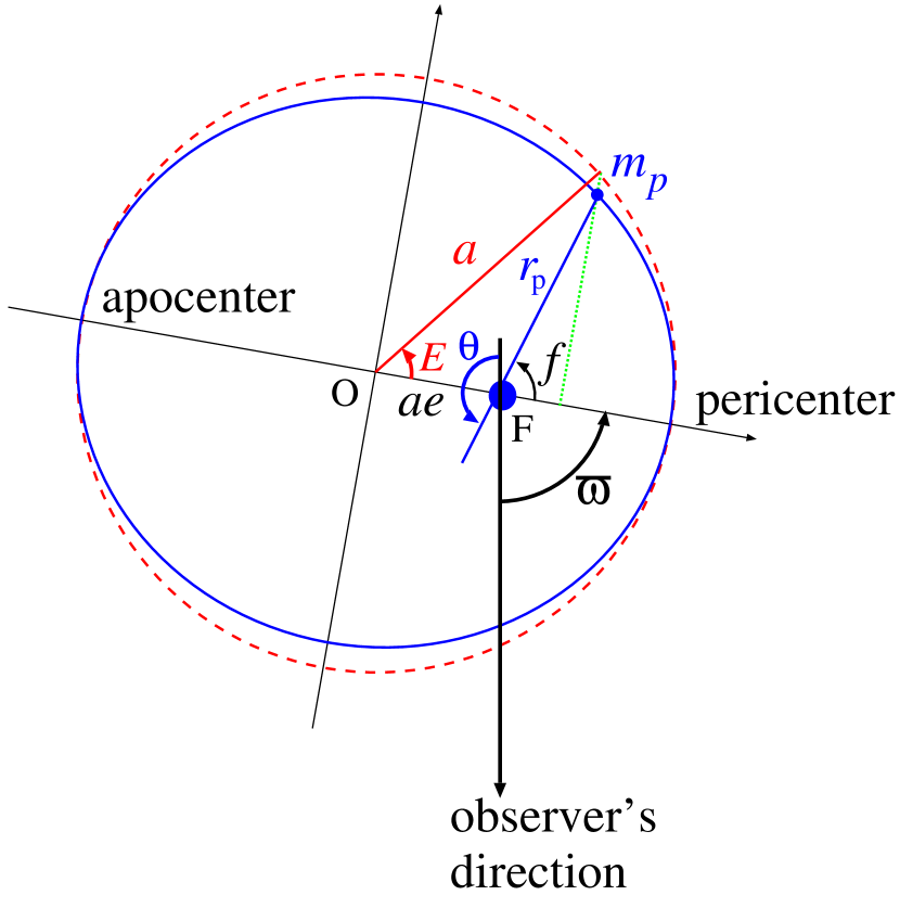
Figure 1: Schematic top view of the planetary orbit. The star is located at the focus point F (see Table 1 for meaning of symbols).

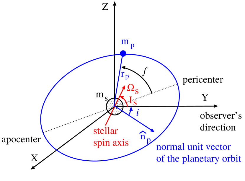
Figure 2: Schematic configuration of the stellar spin axis, the planetary orbital plane, and the observer’s line of sight (see Table 1 for meaning of symbols).

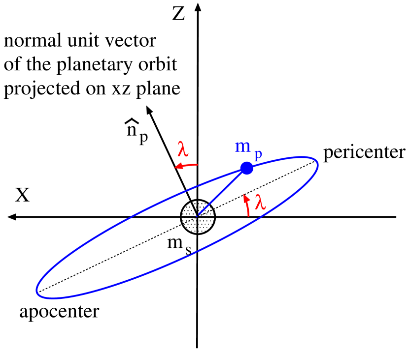
Figure 3: Projected view of the planetary orbital plane from the line of sight ($Y$-axis in this case).

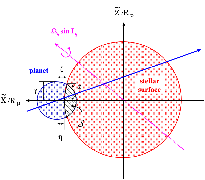
Figure 6: Schematic illustration of the configuration of the system at ingress of the planet in the new coordinates.

Figure 12: Joint probability distribution of the best-fit parameters $(V\sin I_{s},~{}\lambda)$ in the likelihood analysis for the mock HD 209458 observation. We adopt the prior assumption for fiducial parameters (top left), $R_{p}=1.407\,R_{\rm J}$ (top right), $R_{s}=1.196\,R_{\odot}$ (bottom left) and $a=0.0482\,{\rm AU}$ (bottom right). In each panel, the cross indicates the correct values of $(V\sin I_{s},~{}\lambda)$, and the contour levels around it represent the 1 and 2 $\sigma$ levels of the probability distribution. The solid lines projected onto the horizontal and vertical axes represent the probability distributions of $V\sin I_{s}$ and $\lambda$, respectively. Note that all the mock data created in the likelihood analysis assume the parameters listed in Table 2. Thus, except for the top left panel, the difference between the incorrect prior assumption and the correct value for $(R_{p},R_{s},a)$ was used in each panel.

Figure 13: Expected constraints on the spin parameters $(V\sin I_{s},~{}\lambda)$ from the $\chi^{2}$ fit to the mock data of radial velocity curves for the HD 209458 system. The thin and the thick lines show the results obtained from the different mock samples created according to the same parameters, as listed in table 2. The two contour curves in each line width represent the 1 and 2 $\sigma$ confidence levels. The locations of the crosses represent the true values of the spin parameters $(V\sin I_{s},~{}\lambda)$, while the locations of the plus signs indicate the best-fit parameters, which were estimated under the prior assumption for the limb-darkening coefficient and the orbital eccentricity as the corect parameters (top left), $\Delta R_{p}=0.06\,R_{\rm J}$ (top right), $\Delta R_{s}=0.05\,R_{\odot}$ (bottom left), and $\Delta a=1.4\times 10^{-3}\,{\rm AU}$ (bottom right).

References

- Alonso et al. (2004) Alonso, R., Bron, T.M., Torres, G., Latham, D.W. Sozzetti, Al., Mandushev, G., Belmonte, J.A., Charbonneau, D., Deeg, H.J., Dunham, E.W., O’Donovan, F.T., and Stefanik, R.P. 2004, ApJ, 613, L153
- Bouchy et al. (2004) Bouchy, F., Pont, F., Santos, N.C., Melo, C., Mayor, M., Queloz, D., and Udry, S. 2004, A&A, 421, L13
- Brown et al. (2001) Brown, T.M. et al., 2001, ApJ, 552, 699.
- Charbonneau et al. (1998) Charbonneau, D., Jha, S., and Noyes, R. W., 1998, ApJ507, L153.
- Charbonneau et al. (1999) Charbonneau, D. et al., 1999, ApJ522, L145.
- Charbonneau et al. (2000) Charbonneau, D. et al., 2000, ApJ529, L45.
- Claret (2000) Claret, A. 2000, A&A, 363, 1081
- Gizon & Solanki (2003) Gizon, L., & Solanki, S, K. 2003, ApJ, 589, 1009.
- Henry et al. (2000) Henry, G.W. et al., 2000, ApJ, 529, L41.
- Hosokawa (1953) Hosokawa, Y. 1953, PASJ, 5, 88.
- Konacki et al. (2003) Konacki, M., Torres, G., Jha, S. and Sasselov, D. D., 2003, Nature, 421, 507.
- Kopal (1942) Kopal, Z. 1942, Proc. U.S. Natl. Acad. Sci., 28, 133
- Kopal (1945) Kopal, Z. 1945, Proc. Am. Phil. Soc. 89, 517
- Kopal (1990) Kopal, Z. 1990, Mathematical Theory of Stellar Eclipses (Dordrecht: Kluwer).
- Lin et al. (1996) Lin, D.N.C., Bodenheimer, P., Richardson, D.C. 1996, Nature, 380, 606
- McLaughlin (1924) McLaughlin, D. B. 1924, ApJ, 60, 22
- Murray & Dermott (1999) Murray, C.D. and Dermott, S.F., 1999, Solar System Dynamics (Cambridge: University of Cambridge Press)
- Noyes et al. (1985) Noyes, R.W., Hartmann, L.W., Baliunas, S.L., Duncan, D.K., and Vaughan, A.H. 1985, ApJ, 279, 763.
- Petrie (1938) Petrie, R. M. 1938, Publ. Dominion Astrophys. Obs., 7, 133
- Pollack et al. (1996) Pollack, J.B., Hubickyj, O., Bodenheimer, P., et al. 1996, Icarus, 124, 62
- Pont et al. (2004) Pont, F., Bouchy, F., Queloz, D., Santos, N. C., Melo, C., Mayor, M., & Udry, S. 2004, A&A, 426, L15
- Queloz et al. (2000) Queloz, D., Eggenberger, A., Mayor, M., Perrier, C., Beuzit, J.L., Naef, D., Sivan, J.P., and Udry, S., 2000, A&A, 359, L13.
- Rossiter (1924) Rossiter, R. A. 1924, ApJ69, 15.
- Santos et al. (2004) Santos, N.C., Bouchy, F., Mayor, M., et al. 2004, A&A, in press (astro-ph/0408471)
- Schlesinger (1909) Schlesinger, F. 1910 Publ. Allegheny Obs., 1, 123
- Snellen (2004) Snellen, I. A. G. 2004, MNRAS, 353, L1
- Udalski et al. (2002a) Udalski, A., Paczyński, B., Żebrún, K., Szymański, M., Kubiak, M., Soszyński, I., Szewczyk, O., Wyrzykowski, Ł., and Pietrzyński, G., 2002a, Acta Astron.52, 1
- Udalski et al. (2002b) Udalski, A., Żebrún, K., Szymański, M., Kubiak, M., Soszyński, I., Szewczyk, O., Wyrzykowski, Ł., and Pietrzyński, G., 2002b, Acta Astron.52, 115
- Udalski et al. (2002c) Udalski, A., Szewczyk, O., Żebrún, K., Pietrzyński, G., Szymański, M., Kubiak, M., Soszyński, I., and Wyrzykowski, Ł., 2002c, Acta Astron.52, 317
- Udalski et al. (2003) Udalski, A., Pietrzyński, G., Szymański, M., Kubiak, M., Żebrún, K., Soszyński, I., Szewczyk, O., and Wyrzykowski, Ł., 2003, Acta Astron.53, 133
- Winn et al. (2004) Winn, J.N., Suto, Y., Turner, E.L., Narita, N., Frye, B.L., Aoki, W., Sato, B., & Yamada, T. 2004, PASJ, 56, 655