3-D Photoionization Structure and Distances of Planetary Nebulae II. Menzel 1

Abstract

We present the results of a spatio-kinematic study of the planetary nebula Menzel 1 using spectro-photometric mapping and a 3-D photoionization code. We create several 2-D emission line images from our long-slit spectra, and use these to derive the line fluxes for 15 lines, the H$\alpha$/H$\beta$ extinction map, and the [SII] line ratio density map of the nebula. We use our photoionization code constrained by these data to derive the three-dimensional nebular structure and ionizing star parameters of Menzel 1 by simultaneously fitting the integrated line intensities, the density map, and the observed morphologies in several lines, as well as the velocity structure. Using theoretical evolutionary tracks of intermediate and low mass stars, we derive a mass for the central star of 0.63 $\pm$0.05M_⊙. We also derive a distance of 1050 $\pm$150pc to Menzel 1.

1 Introduction

The Planetary Nebula (PN) Menzel 1 (Mz 1) or G322.4-02.6 (15^h 34^m 16^s.7 -59^o 08’ 59” 2000.0) is a bright object with a bipolar morphology and a prominent central ring of enhanced emission. H$\alpha$ and [OIII] narrow band images of Mz 1 have been published by Schwarz, Corradi, & Melnick (1992). Being bright has not resulted in Mz 1 being well-studied; only a few papers have been dedicated to the object.

H₂ emission has been detected from Mz 1 by Webster, Payne, Storey, Dopita (1988) and the morphology in this molecular line is similar to that of our optical image, shown in Fig. 1.

A detailed kinematical study of Mz 1 was done by Marston, et al. (1998) using high resolution echelle spectroscopy. Using the intensity ratio of the [SII] lines they computed densities of 1700 $cm^{-3}$ for the main ring and 400 $cm^{-3}$ for the bipolar part. They show that the gas in the main part of the nebula is expanding at 23 $km\,s^{-1}$, and that the velocity structure is consistent with a cylindrical model with expansion velocities proportional to the radial distance from the center. They also show that the dynamical age of the ring in Mz1 is of the order of 7000 yrs and estimate a mass of about 0.5M_⊙ for the nebula using dynamical arguments and their computed distance of 2.0 kpc.

Distances have been determined by several authors such as Van de Steene, & Zijlstra (1995) with 2.53 kpc, Cahn, Kaler, & Stanghelini (1992) with 2.28 kpc and Zhang (1995) with 2.85 kpc, all using statistical methods and based on the same data. Using the same formalism as Van de Steene, & Zijlstra (1995) and a new value for the radius of the nebula, Marston et al. (1998) obtained a distance of 2.0 kpc with a claimed uncertainty in this estimate of about 30%. Acker et al. (1992) lists 10 distances of which 8 are statistical and 2 individual determinations. Given that all the above authors use a filling factor, $\epsilon$ = 0.5, any such method has an inherent and large uncertainty in the distances they determine. We compute 2.0 $\pm$0.5 kpc (adjusted standard deviation) from all 14 literature distances without any weighting factor. Note that each individual distance can be in error by a large factor (see the appendix), and the standard deviation computed from the literature values is not very robust.

An effective temperature of 139 kK and a luminosity of 147 L_⊙ were determined by Stanghellini, Corradi, Schwarz (1993) with a distance of 1.8 kpc. Mz 1 is clearly under-luminous for a typical PN.

In this work we present observations of, and a 3-D photoionization model for Mz 1, and derive the 3-D structure of the PN constrained by observed fluxes and morphologies in many emission lines, using the same method as Monteiro, Schwarz, Gruenwald, & Heathcote (2004) applied to NGC 6369. By determining the 3-D structure of nebulae, the large uncertainty involved in all classical statistical distance determination methods is eliminated. Assuming an arbitrary filling factor, constant ionized mass or diameter, mass-radius relationship etc. is not needed here: we determine what the structure and ionized mass are, and can therefore derive distances to much greater accuracy than has been previously possible.

In summary, we obtain the 3-D spatial structure of the nebula along with its chemical composition, ionizing source temperature, luminosity, and mass, as well as an independent distance, in a self-consistent manner. In §2 we discuss the observations and briefly explain the basic reduction procedures, including our image reconstruction technique used to obtain the emission line intensity images. In §3 the results obtained from these images are discussed: the pixel by pixel reddening correction of the images, the integrated line fluxes, and the computed temperature and density maps. In §4 we present the model results generated by our 3-D photoionization code, and we discuss the derived quantities. In §5 we give our conclusions, and explain in detail how our method works in the appendix.

2 Observations

2.1 Observations and data reduction

We show our image of Mz 1 in Fig. 1 taken in the light of the [SII]671.7nm line through a filter with $\lambda_{c}$ = 671.8nm and FWHM = 2.6 nm. The 300 s exposure was taken with the CCD camera attached to the CTIO 0.9m telescope on the 9th of April 2002. The plate-scale is 0.4″/pix on the 2kx2k TEK chip, and the seeing during the exposure was  1.1″ according to the nearby seeing monitor.

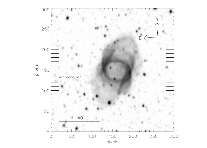
Figure 1: Our narrowband [SII] image of Mz 1 with the scale and orientation indicated. We have indicated the centers of the slit positions we used by the short strokes on both sides of the image.

The main features of this [SII] image are similar to those found in the H$\alpha$ image of Schwarz, Corradi, & Melnick (1992). The morphology of Mz 1 is complex: two faint outer lobes toward the NW and SE meet in the brighter central annular region, and there are enhanced extended bands of emission on the eastern and western side of the central annulus. Some fine structure is also seen throughout the surface of the nebular emission.

The spectra were taken with the CTIO 1.5 m Ritchey-Chrétien telescope with the RC Spectrograph on the nights of 13 and 14th June, 2002. We used a grating with 600 l/mm blazed at 600 nm giving a spectral resolution of 0.65 nm/pixel and a plate scale of 1.3″/pixel with a slit width of 4″. The spectral coverage obtained with this configuration was approximately 450 nm to 700 nm. For details of the instrument and telescope see http://www.ctio.noao.edu and click on “Optical Spectrographs”, then on “1.5m RC spectrograph”.

By taking exposures at several parallel long-slit positions across the nebula, we obtained line intensity profiles for each slit. These profiles were then combined to create emission line images of the nebula with a spatial resolution of about $4\arcsec\times 4\arcsec$, in a way similar to radio mapping. Due to a technical problem the data from one of the observed slit positions had to be discarded. We computed an average of the two adjacent slit spectra as representing this position (shown in Fig. 1). The added uncertainties introduced by this procedure are discussed below.

The individual slits were observed and reduced using standard procedures for long-slit spectroscopy, using IRAF reduction packages.

A fine correction for slit misalignment was made using the H$\alpha$ and H$\beta$ profiles for each exposure. Using IDL, the images were re-dimensioned to 100 times their original size. The normalized H$\alpha$ and H$\beta$ profiles were then matched and the final result re-dimensioned to original values. This procedure yields the precise alignment necessary for calculation of diagnostic line intensity ratios. Minor shifts of the order of one pixel can introduce considerable errors in line ratios, if this method is not applied.

It is also important to note that the 11 slit positions observed do not fully cover the nebula, leaving out the faintest outer parts of the bipolar lobes; see Fig. 1. Below we estimate this lost flux and show that it is a small fraction of the total flux. Note, however, that in our calculations, we take this “lost flux” into account by matching our model output fluxes to the observed area, but the model does provide the complete nebular structure.

3 Observational results

Images were created for all 15 lines detected with a signal-to-noise ratio above 5. In Fig. 2 the constructed images for the most important emission lines are shown. These images have been corrected for reddening as described in the following section. The corresponding signal-to-noise images were used to obtain the total line intensities with fractional errors, given in Table 1.

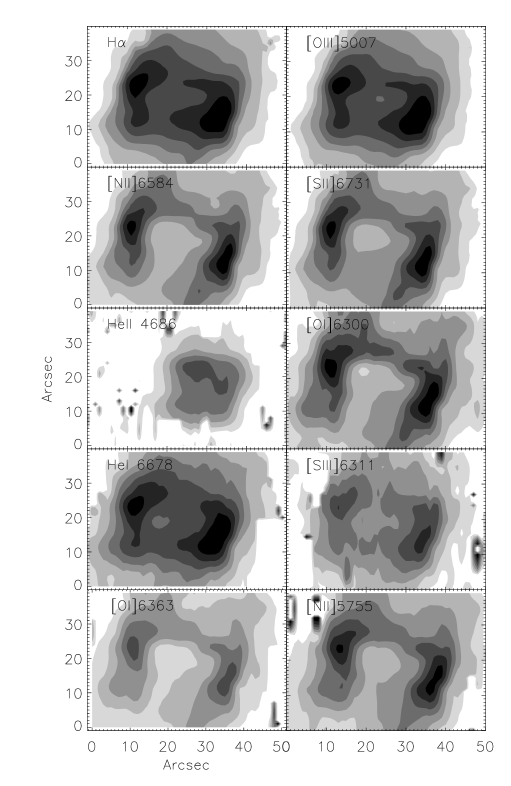
Figure 2: Reddening corrected emission line images for Mz 1. Only the 10 images with the highest S/N are shown.

3.1 Reddening correction and total fluxes

From our long-slit spectra we reconstruct emission line images using the method described by Monteiro, Schwarz, Gruenwald, & Heathcote (2004). These images for each line were corrected for reddening using the H$\alpha$/H$\beta$ ratio map shown in Fig. 3. The logarithmic correction constant was calculated pixel by pixel using the theoretical value of H$\alpha$/H$\beta$=2.87 from Osterbrock (1989) and the reddening curve of Seaton (1979).

We investigated the effect of differential atmospheric refraction on this ratio map. From the airmasses of our observed positions and the values given by Filippenko (1982) we computed a correction which we applied to our data. All slit positions were observed at airmasses below 1.5 except one outer position in a faint part of the nebula, which had an airmass of 1.8. Since we used a 4″wide slit and the object is extended, the effect was small, but not negligible in the steep gradients near the bright ring structure. The average error due to this effect is about 3% in the high signal to noise (S/N) areas and about 25% in the low S/N areas. The nett effect on the final calculated relative total fluxes is about 0.3% for strong lines and 7% for weak ones, well within the other observed uncertainties.

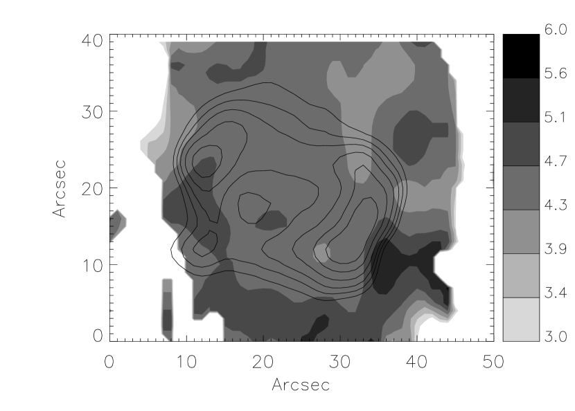
Figure 3: The Mz 1 H$\alpha$/H$\beta$ ratio map with contour overlay of H$\alpha$, where the darker shading represents stronger emission. Only the brighter parts of the nebula are shown as the image is cut for S/N values lower than 10.

The final calculated line fluxes relative to H$\beta$ and their corresponding 1$\sigma$ errors are shown in Table 1. All total fluxes were obtained by integrating the reddening corrected images pixel by pixel. The value we obtained for the total reddening corrected H$\beta$ flux is $F_{H\beta}\,=\,2.6\times 10^{-11}erg\,cm^{-2}\,s^{-1}$. We estimate from the relative area of the nebula that falls outside the slit images, and the fact that for several lines the flux comes mainly from the central, bright part of Mz 1, that the lost flux in $H\beta$ is about 3% of the total, and the average lost flux in all lines about 5%. Note that Acker et al. (1992) lists an uncorrected H$\beta$ flux of 4.9$\times 10^{-12}erg\,cm^{-2}\,s^{-1}$, taken from Perek (1971), which is close to our uncorrected value of 5.8$\times 10^{-12}erg\,cm^{-2}\,s^{-1}$. Our flux is obtained digitally by integrating our spectrophotometry pixel by pixel over the whole nebula, while Perek used photoelectric aperture photometry during non-photometric nights, with all its associated calibration problems, and warns us in his article that cirrus affected many of the measurements, explaining why his flux is lower than ours which was taken during a photometric night. Perek also listed a previous measure of the H$\beta$ flux of -11.26 which is equal to our uncorrected flux.

Table 1: Line fluxes relative to H$\beta$

Line $\lambda$(nm)	Flux	Dered. Flux	Error (%)
HeII$\lambda$468.6	0.11	0.11	7
[OIII]$\lambda$495.9	2.35	2.28	6
[OIII]$\lambda$500.7	7.11	6.83	6
[NII]$\lambda$575.5	0.10	0.07	23
HeI$\lambda$587.6	0.25	0.16	9
[OI]$\lambda$630.0	0.33	0.21	8
[SIII]$\lambda$631.1	0.03	0.02	20
[OI]$\lambda$636.3	0.12	0.08	14
[NII]$\lambda$654.9	2.96	1.81	12
$H\alpha$	4.68	2.88	6
[NII]$\lambda$658.4	9.18	5.57	12
HeI$\lambda$667.8	0.08	0.05	15
[SII]$\lambda$671.7	0.82	0.49	12
[SII]$\lambda$673.1	0.76	0.45	12

Using these images we estimated the effect of adopting the average for the discarded slit position. Since the nebula shows considerable symmetry, we compared the northern half of the reconstructed images with the southern half. By comparing the total fluxes from these halves we determined that the error on the calculated total fluxes were about 10% for low ionization lines and about 2% for the other ones. This difference is due to the fact that the discarded position is close to the bright ring of the nebula, where the low ionization lines are relatively strong. The effect is relatively small and this added uncertainty is taken into account in the values presented in Table 1.

3.2 Gas density and temperature

We calculated density and temperature maps from the reddening corrected maps of the [SII] and [NII] lines respectively. The expressions relating the line intensity ratios to the gas density and temperature are the ones published by McCall (1984) and those used in the IRAF temden package. Details are as in Monteiro, Schwarz, Gruenwald, & Heathcote (2004). The density map is shown in Fig. 4.

For the temperature maps, the correction for slit misalignment was carried out as done for the H$\alpha$/H$\beta$ maps discussed in section 2.1. We compute the temperature map for Mz 1 in two ways: using our density map we obtain the temperature map shown in Fig. 5 (A) and in (B) we show the difference between this map and the one calculated assuming constant density. The maximum difference between these two maps is less than 100 K. The images are clipped for data values with S/N lower than 10 for visual clarity.

Figure 4: Density map obtained from the [SII]671.7,673.1nm line ratio.

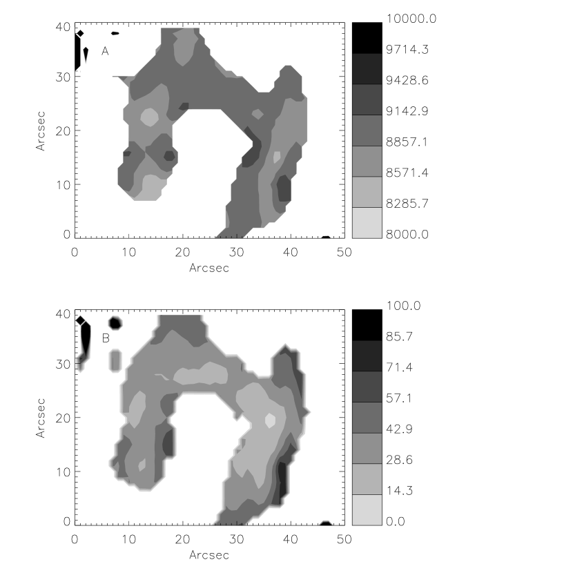
Figure 5: (A) Temperature map obtained from the de-reddened [N II] line ratio. The scale on the right is in degrees centigrade; (B) difference between this map and the one obtained assuming constant density. Note that the maximum difference is less than 100 K. North is up, and east is to the left.

4 Photoionization Models

The photoionization code applied here has been described in detail by Gruenwald, Viegas, & Broguière (1997). It uses a cube divided into cells, each having a given density, allowing arbitrary density distributions to be studied. Typical models runs use cubes of 70 to 100 cells on a side. The input parameters are the ionization source parameters (luminosity, spectrum, and temperature), elemental abundances, density distribution, and the distance to the object. The conditions are assumed uniform within each cell for which the code calculates the temperature and ionic fractions. These values are used to obtain emission line emissivities for each cell.

The final data cube can be spatially oriented and projected in order to reproduce the observed morphology. The orientation on the sky of the 3–D nebular structure is thus determined. The line intensities and other relevant quantities are then obtained after projection onto the line of sight.

The structure we obtained for Mz 1 is shown in Fig. 6 as it is oriented relative to the observer. We also show a cut along the major axis of symmetry in Fig. 7, indicating the density values. The 3–D structure of Mz 1 was constrained by our density map to be an open structure, not a closed shell of any type. We therefore adopt an hour-glass shape with a density gradient from the equator to pole. We added random density fluctuations to better fit the line fluxes, especially H$\beta$. The rotation angles relative to the x, y, and z axes respectively, are 0^o,10^o, and 40^o, with the symmetry axis of the main hour-glass structure being x. The model resolution of $100^{3}$ cells was limited by our 4 GB of computer memory, and code execution time.

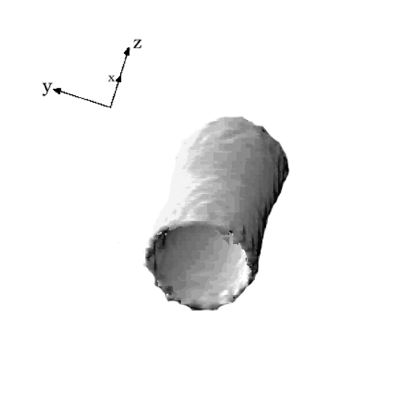
Figure 6: Isocontour plot of the 3-D density structure determined for Mz 1 using model calculations. The inclination angle of the polar axis of the structure is 40^o.

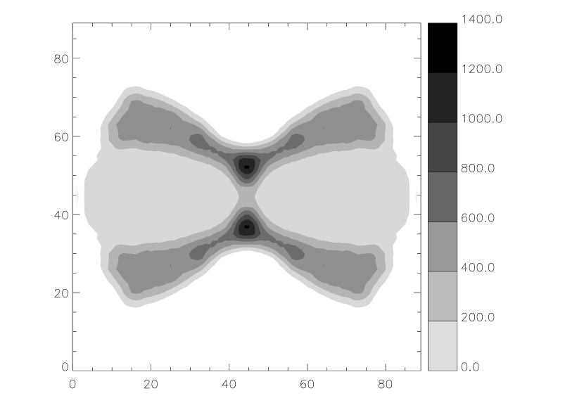
Figure 7: Cut of the density structure of Mz 1 determined by the model calculations.

The ionizing spectrum we used for the central star (CS) was a blackbody modified by the He and H atomic absorption edges at 54.4eV and 13.6eV. The addition of these edges was necessary to be able fit the [OIII] and HeII line intensities simultaneously, the HeII line being particularly sensitive to the depth of the absorption edge, and therefore providing a good central star temperature constraint. These absorption edges are also present in the more sophisticated theoretical atmospheric models presented by Rauch, Deetjen, Dreizler & Werner (2000), which are similar to the ones we used here for similar stars. The only feature from Rauch’s spectra that we do not incorporate is the added absorption due to other lines, but this has no significant effect on our model. The effective temperature and luminosity of our adopted crude stellar spectrum are given in Table 2.

4.1 Model Results

We present here the main results obtained from the photoionization model constrained by the observational data. The total line intensities are given in Table 2, as well as the fitted abundances and ionizing star parameters. Projected line images for four important transitions are shown in Fig. 8.

The model image size is fitted to the observed one for the line [NII]658.4nm, as well as the absolute $H\beta$ flux, giving a final distance of 1050$\pm$150 pc. Fig. 9 shows the observed [NII] image with the corresponding model image contours overlaid for the obtained distance.

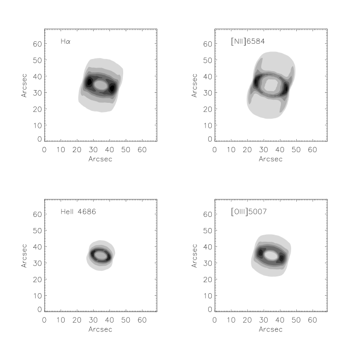
Figure 8: Projected line images obtained with the photoionization model.

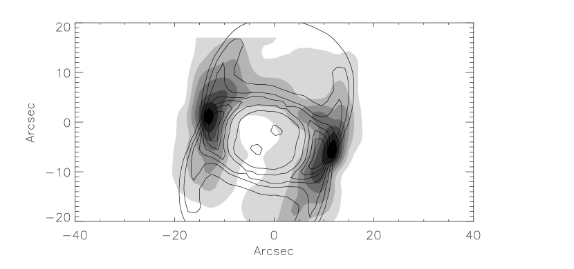
Figure 9: Contour image of model [NII] image overplotted on observed image for our best distance of d=1050$\pm$150 pc.

Table 2: Observed and model line fluxes and model central star parameters.

	Observed	Model
$T_{*}$ (K)		120kK
$L_{*}/L_{\odot}$	-	164
Density	100-1400	100-1400
He/H	-	$1.14\times 10^{-1}$
C/H	-	$3.3\times 10^{-4}$
N/H	-	$2.2\times 10^{-4}$
O/H	-	$4.7\times 10^{-4}$
Ne/H	-	$3.5\times 10^{-4}$
S/H	-	$1.1\times 10^{-5}$
log($H\beta$)	-10.6	-10.6
[NeIII]386.8a	5.64	4.8
HeII468.6	0.014	0.013
[OIII]500.7	6.83	6.68
HeI587.6	0.16	0.17
[OI]630.0	0.21	0.26
[NII]658.4	5.6	5.3
[SII]671.7	0.49	0.49
[SII]673.1	0.45	0.46

a) Value obtained by Kaler, Shaw, Browning (1997)

Using the model cube of temperatures and ionization structure we also calculated the position-velocity (PV) diagram for four different slit positions using a spherically symmetrical velocity field given by $\vec{V}=\alpha(\left|\vec{r}\right|/rmax)\times\vec{r}/{\left|\vec{r}\right|}$ . r_max is half the side of our model data cube (here we used r_max = 8 10¹⁷ cm), and $\alpha$ is the maximum velocity reached within the data cube (here we used 45 km/s). We computed the PV diagram for the [NII]658.4nm line in the same positions as those observed by Marston et al.(1998). The projected velocities in the $x$ direction are obtained using:

$$\phi_{\lambda}(v,y,z)=\sum_{x}{{\epsilon_{\lambda}(x,y,z)}\over{\sqrt{\pi}.\xi(x,y,z)}}.e^{-{[{{\Delta V(v,x,y,z)}\over{\xi(x,y,z)}}]}^{2}}~{}~{}~{}~{}~{}~{}~{}~{}~{}~{}~{}~{}~{}~{}~{}~{}(1)$$

with:

$$\Delta V(v,x,y,z)=V_{x}(x,y,z)-v~{}~{}~{}~{}~{}~{}~{}~{}~{}~{}~{}~{}~{}~{}~{}~{}~{}~{}~{}~{}~{}~{}~{}~{}~{}~{}~{}~{}~{}~{}~{}~{}(2)$$

$$\xi(x,y,z)=\sqrt{V_{th}^{2}(x,y,z)+V_{T}^{2}}~{}~{}~{}~{}~{}~{}~{}~{}~{}~{}~{}~{}~{}~{}~{}~{}~{}~{}~{}~{}~{}~{}~{}~{}~{}~{}~{}~{}~{}~{}~{}~{}(3)$$

$$V_{th}(x,y,z)=\sqrt{2kT_{e}(x,y,z)/Am_{H}}~{}~{}~{}~{}~{}~{}~{}~{}~{}~{}~{}~{}~{}~{}~{}~{}~{}~{}~{}~{}~{}~{}~{}~{}~{}~{}~{}~{}(4)$$

where $\epsilon_{\lambda}(x,y,z)$ is the emissivity of a cell at $(x,y,z)$, $V_{T}$ is the turbulent velocity (taken to be 2 km/s) and $V_{th}(x,y,z)$ the thermal velocity of an atom of atomic mass A, the local electron temperature is $T_{e}(x,y,z)$, and v is the plotting interval for the velocity, where in this case v goes from -80 to +80 km/s. m_H is the mass of an H atom. The PV diagram obtained is shown in Fig. 10.

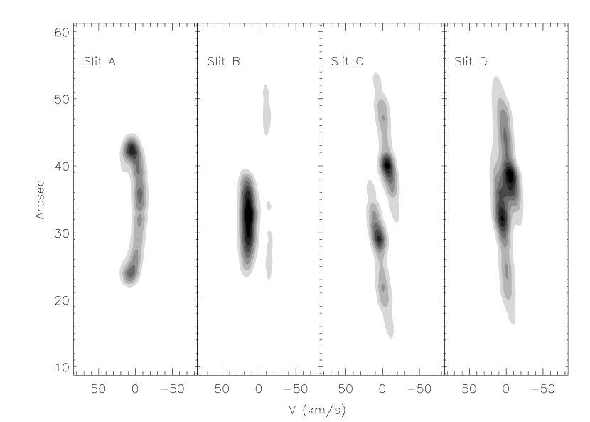
Figure 10: Model PV diagram obtained for the four slit positions as observed by Marston, et al. (1998) in the light of the [NII]658.4 nm line.

Comparing our model derived PV diagrams with the observed ones in Figure 3 of Marston et al.(1998) we see a remarkable agreement. The main features are reproduced, confirming our confidence in the 3-D structure we adopted for Mz 1.

5 Discussion and conclusions

We present spectrophotometric maps of Mz 1, giving spatially resolved information for many emission lines and precise total fluxes for the observed part ($\geq$95% of the total flux) of the nebula. The images produced with this technique were used to determine properties of the nebula using the H$\alpha$/H$\beta$ ratio map for the de-reddening, the [SII] line ratios for the density, and the [NII] line map for the temperature.

The H$\alpha$/H$\beta$ map shows little structure. The prominent ring feature of the nebula does not show significant differences in extinction when compared to the other regions. This may imply that most of the reddening is due to the foreground, and not intrinsic to the nebula.

We also show the density map obtained from the observations indicating the presence of a dense waist ring and a bipolar structure of lower density. Based on this map we propose for Mz 1 a 3–D hour-glass structure with a waist whose density decreases smoothly from the equator to the poles.

Using a photoionization code and the proposed structure we obtained a complete 3–D physical model for Mz 1. The fitted model line intensities show excellent agreement –well within the computed errors– with the observed values. The obtained distance of d=1050$\pm$150 pc falls near the lower end of the error range determined from 14 literature values for the distance. This makes sense as the angular radius of 25″ used in the statistical methods is smaller than the true size of the nebula of 38″  as measured by Schwarz, Corradi, & Melnick (1992), and our distance is also smaller.

The luminosity of 164 $\pm$ 25 L_⊙ and temperature of 120 $\pm$ 16 kK we have determined for the central star are within their errors equal to those found by Stanghellini, Corradi, Schwarz (1993), taking into account the difference in distance and total flux. Our errors have been conservatively estimated to be similar to the cumulative observational errors we computed and used to constrain the model. This luminosity is low for a PN CS, and indicates that the star is evolved and well down its Schönberner track, as confirmed by its position in Fig. 11.

Figure 11: Comparison of our model temperature and luminosity obtained for the central star with model tracks calculated by Blöcker (1995).

We determine the mass of the CS to be 0.63 $\pm$0.05M_⊙ by fitting to the theoretical evolutionary tracks of Blöcker (1995) , using the errors estimated from our observational data and propagated to the CS luminosity and temperature. Due to the fact that in this part of the HR diagram, the tracks lie close together, we cannot say with any precision what the precursor mass of this star was, except to place a lower limit on this mass of about 1 M_⊙ using the added track from Vassiliadis, & Wood (1994) in Fig. 11. The likely value for the CS precursor mass is about 3M_⊙, based on the most probable CS mass of 0.63 M_⊙. From our model output we compute the ionized nebular mass to be 0.14 $\pm$0.03 M_⊙.

An independent check is the time scale of expansion of Mz1. From Marston, et al. (1998) and scaling to our distance we get an expansion time of 3500 yrs for the ring which can be longer or shorter depending on what the history of the expansion has been -decreasing velocity due to energy conservation in a wind blown cavity would shorten the time and increasing velocity due to expansion into a medium with decreasing density would lengthen it-so a range of about 2000-5000 yrs. For the outer parts of Mz1 this time would be about 4700-12000 yrs as the material has had to travel 2.4 times further away from the CS (38″ instead of 16″). From our luminosity range and computing Blöcker track ages we obtain 4500 to 10000 yrs, quite compatible with the outer nebular expansion time, thus confirming our distance determination.

Since the sum of the ionized nebular mass and the CS mass is 0.77 M_⊙, we expect that there possibly is more than 2 M_⊙ of neutral matter near Mz 1. Clearly, for the lower CS precursor mass limit of 1 M_⊙, the neutral mass estimate is a factor of ten smaller. In any case, there is likely more neutral than ionized mass in the system. Note, however, that Huggins, Bachiller, Cox, Forveille (1996) estimate a molecular mass of 0.0086 M_⊙ and an ionized mass of 0.027 M_⊙. They used a radius for Mz1 of 12.6″ instead of the 38″ optical radius, so naively assuming that the mass scales as the third power of the radius would increase their ionized mass by a factor of up to 9 to 0.25 M_⊙, which is much closer to our computed mass of 0.14 M_⊙.

We have put together the Spectral Energy Distribution (SED) from 0.36 to 100 $\mu$m for Mz 1, using data from the literature listed in SIMBAD. The plot of $\lambda\,F(\lambda)$ is shown in Fig. 12. Note that the 100 $\mu$m IRAS point is an upper limit. The double peaked distribution is typical for a PN.

Figure 12: The SED for Mz 1 between 0.44 $\mu$m and 100 $\mu$m using flux values taken from the literature.

Integrating our SED yields a luminosity of about 60 L_⊙ which includes the usual correction proposed by Myers et al. (1987) of a factor of 1.5. This implies that about 60% of the UV radiation from the CS escapes from the nebula. Given that the structure we found is open toward the poles, and is likely clumpy, this is a reasonable value. The fact that we estimate that there is between 0.2 and 2 M_⊙ of neutral matter around Mz 1, some of this may have, in fact, become ionized due to this escaping radiation. Searching for a large, low surface brightness halo around Mz 1 may therefore be useful.

Perhaps most important is the fact that our simple method can be applied to any spatially resolved emission line nebula, yielding the complete 3–D structure and an accurate distance. The time consuming multiple position long slit observations can be dispensed with since Integral Field Spectrographs are now becoming available at major observatories, making the method not just simple but also efficient. See the detailed explanation of our method in the appendix.

6 Appendix: Determining distances using 3-D photoionization models

Classical distance determination methods are statistical or individual in nature and all assume constancy of one or more physical parameters of the PNe. Gurzadyan (1997) provides an excellent review of distance determination methods and we refer to his book for details on other methods than the “Astrophysical Method” (AM) which is the one we use here.

The AM uses the fact that the electron density, H$\beta$ flux, and angular extent are observable quantities of PNe –treated as spherically symmetrical objects– and that they are related to the distance of the nebula by:

d = 2.4.10²⁵ F(H$\beta$)/[n² . $\theta^{3}$ . $\epsilon$]                                                  (5)

where F(H$\beta$) is the H$\beta$ flux in ergs/cm²/s, n² is the electron density in cm^-3, $\theta$ is the observed angular extent of the nebula, and $\epsilon$ is the so-called filling factor which is the fraction of the nebular volume which is emitting i.e. it contains ionized gas.

It is therefore in principle possible, if all the above parameters are known, to determine an accurate distance to any resolved, spherical nebula or HII region. In practice, however, the method has severe limitations due to the necessity of restrictive assumptions such as spherical symmetry. Taking each parameter in turn, we show that a typical distance determination has an error of about a factor of 3 or more for any given nebula. There are nebulae for which individual distances with a range of a factor of 100 have been published (M2-9 extremes are: 50 to 5200 pc; Schwarz, Aspin, Corradi, & Reipurth (1997))!

H$\beta$ fluxes are typically measured in a small aperture centered on the PN, and an attempt is made to estimate the flux from the entire nebula by extrapolation. Typical errors are large due to incomplete knowledge of the size and brightness structure of the nebulae. The presence of the central star in the aperture increases the uncertainty in this measurement. Estimated errors are in the range 1.5 for smooth, regularly shaped nebulae without much structure to 3 or more for more typical PNe.

Electron densities, n, are usually determined from the ratio of the pair of forbidden sulfur lines at 671.7 and 673.1nm. Since spectra are also typically taken with small apertures centered on the PN or in the best cases with a long slit but for only one position across the nebula, again the uncertainty in the average value of n is large, say, a factor of 1.5-2. Note that n appears in the equation to the second power, increasing the effect of this error.

The angular extent, $\theta$, of a nebula can be measured but depends on the passband or emission line used to make the observations. A PN can have a diameter in the light of the [NII] line that is twice that measured in H$\beta$ or [OIII], again producing uncertainties in the distance determination. Smaller nebulae have a correspondingly larger uncertainty associated with this measurement. $\theta$ appears in the equation to the third power, increasing the effect of the uncertainty in this parameter. An error of about a factor of 1.5 - 3 is again typical. In any case, the use of the radius assumes spherical symmetry, which for most PNe is far from realistic.

The most difficult to determine and therefore least known parameter is the filling factor, $\epsilon$. Usually, it is taken to be 0.5 in statistical methods using large samples of nebulae, but the true value can be anywhere between 0 and 1, with typical estimates varying between 0.2 and 0.9, i.e. a factor of about 5 uncertainty.

Propagating all these factors, it is clear that determining a distance to a PN is a very uncertain business.

Our method differs fundamentally from the classical methods, in which one or more of the above parameters were assumed to be constant or have some simple relationship. The use of a 3-D structure to model the nebula eliminates the need for assumptions on the quantities $n$,$\theta$, among others, as the structure can be modified to include small scale variations in density such as clumps, filaments and others as well as large scale variations (hour-glass shapes for example). More importantly, this procedure removes entirely the need to specify a filling factor $\epsilon$, as the large and small scale density variations are all well defined in the 3-D structure. We also determine all of the observables with high precision from either long slit or Integral Field Unit (IFU) spectra across the nebula. Our photoionization model is then constrained by the quantities derived from these detailed spectra, and spectral images. We constrain simultaneously with: several line images, several line fluxes, complete projected density map, and the velocity structure, obtaining the best overall fit by adjusting the central star luminosity, spectral distribution, temperature, average chemical abundances, and the distance, also obtaining the complete and detailed 3-D structure of the nebula. All the above mentioned parameters are therefore known much more precisely, and the distance determination is correspondingly better. Typically we can compute the distance to about 10-20% depending mainly on the observational errors.

6.1 Model fitting procedure

The details of the numerical photoionization code are given in the appendix of Gruenwald, Viegas, & Broguière (1997). In summary, the gaseous region, with the radiation source in the center, is divided into cubic cells, for each of which the physical conditions are, by definition, homogeneous. In each cell thermal and ionization equilibrium is assumed in order to obtain the physical conditions. The radiative transfer problem is calculated with the “on the spot” approximation to save computing time.

The input parameters are the elemental abundances, the gas density distribution, the shape and intensity of the central ionizing radiation spectrum (temperature, H and He absorption edges, and luminosity in the case of a star) and the distance to the object. The code then provides the physical conditions in each point of the nebula, i.e., ionic fractional abundances, electronic temperature and density, as well as the emission line luminosities of each cell.

This output is then used to produce projected images and total fluxes for a given number of emission lines and a set of (x,y,z) orientation angles. This output can then be tailored to match given observational configurations such as single long slits, or multiple slits (as is the case for Mz1). From the projected images we can also construct projected diagnostic maps, such as density and temperature maps.

The model generated or simulated “observations” discussed above are then compared to the actual observational data obtained (in this case, the spectro-photometric mapping of Mz1). We compare total line intensities and check for discrepancies. If one or more of the intensities are out of the range of the observational errors, we proceed to fine tune input parameters that have influence on the given line. For example, we take the $H\beta$ total fluxes from the model and observations and compare them. The $H\beta$ line is mainly dependent on the star luminosity and the 3-D structure of the gas, so we adjust these input parameters accordingly. In this case it is important to realize that the 3-D structure is actually defined by the density in each cell and a physical size for the object which is dependent on the distance. So in fact we are dealing with two input parameters when we consider the $H\beta$ flux. The same type of comparison is made for other lines such as [OIII]500.7nm which is an important coolant, HeII468.6nm which depends mainly on the CS temperature, among others. We also compare the model projected images and diagnostic maps to those obtained from the observations.

After fitting all the model constraints to their respective observational counterparts and adjusting the input parameters of the code accordingly, we calculate a new model. The same procedure discussed above is then repeated until we reach a satisfactory agreement between model and observations for all line images, fluxes, diagnostic maps, etc.

Notice that, after this iterative procedure, we obtain model fitted values for the input parameters that are self-consistently determined; they are the ionizing star characteristics, gas chemical abundances, density, structure, and distance.

One of the main differences of this procedure when compared to previous model calculations in the literature, is that we use the distance as a fitting parameter for the model. This is possible because we now have a way of producing projected images from the 3D model results and can therefore compare them directly with observed ones as well as the observed total fluxes. In other words, we do not use a fixed distance for our model calculations and vary only star and gas parameters (luminosity and temperature of the star, abundances and densities of the gas). The other important advantage of using the 3-D structure for the gas is the possibility of eliminating the need for a “filling factor”. This has major implications on the model parameters that can be determined, especially on the distance.

Since we use a 3-D structure that is consistent with observed images, position-velocity diagrams, diagnostic ratios (such as density maps) we are not making any assumptions about filling factors, ionized masses or physical sizes. All these parameters are determined self-consistently in the model.

The uniqueness of the solution obtained by this procedure can be argued of course. It is immediately clear that within the observational uncertainties there are an infinite number of solutions that can fit the observations. In other words, the observations determine the quality of the final parameters. In fact, if we estimate the goodness of fit of our model fit by quadratically summing all uncertainties and dividing by the number of observables minus the number of degrees of freedom (input parameters to the model), we get an error of about 20% in the case of Mz1. This is the uncertainty adopted for our results. The precise determination of fitting errors is extremely complex and given the nature of the 3-D code neither practical nor useful.

For the above reasons our distance determinations are fundamentally different from, and much more precise than classically found distances.

References

- Acker et al. (1992) Acker, A., Ochsenbein, F., Stenholm, B., Tylenda, R., Marcout, J., Schohn, C. 1992, Strabourg-ESO Catalogue of Galactic PNe.
- Blöcker (1995) Blöcker, T. 1995, A&A, 299, 755
- Cahn, Kaler, & Stanghelini (1992) Cahn, J.H., Kaler, J.B.; & Stanghelini, L. 1992, A&AS, 94, 399
- Filippenko (1982) Filippenko, A. V. 1982, PASP, 94, 715
- Gruenwald, Viegas, & Broguière (1997) Gruenwald, R., Viegas, S. M., & Broguière, D. 1997, ApJ, 480, 283
- Gurzadyan (1997) Gurzadyan, G.A. 1997, “The Physics and Dynamics of Planetary Nebulae”, p.268, Springer.
- Huggins, Bachiller, Cox, Forveille (1996) Huggins, P.J., Bachiller, R., Cox, P., Forveille, T. 1996, A&A, 315, 284
- Kaler, Shaw, Browning (1997) Kaler, J.B., Shaw, R.A., Browning, L. 1997, PASP, 109, 289
- Marston, et al. (1998) Marston, A.P., Bryce, M., López, J.A., Palmer, J.W., Meaburn, J. 1998, A&A, 329, 683
- McCall (1984) McCall, M. L. 1984, MNRAS, 208, 253
- Monteiro, Schwarz, Gruenwald, & Heathcote (2004) Monteiro, H., Schwarz, H.E., Gruenwald, R., & Heathcote,S.R. 2004, ApJ, 609,194
- Myers et al. (1987) Myers, P. C.; Fuller, Gary A.; Mathieu, R. D.; Beichman, C. A.; Benson, P. J.; Schild, R. E.; Emerson, J. P. 1987, ApJ, 319, 340
- Osterbrock (1989) Osterbrock, D. E. 1989, Research supported by the University of California, John Simon Guggenheim Memorial Foundation, University of Minnesota, et al. Mill Valley, CA, University Science Books, 1989, 422 p.,
- Perek (1971) Perek, L. 1971, Bull.Astr.Inst.Cz., 22, 103
- Rauch, Deetjen, Dreizler & Werner (2000) Rauch, T., Deetjen, J. L., Dreizler, S. e Werner, K. 2000, Asymmetrical Planetary Nebulae II: From origins to microstructures, ASP Conference Series 199, 337
- Schwarz, Corradi, & Melnick (1992) Schwarz, H. E., Corradi, R. L. M., & Melnick, J. 1992, AApS, 96, 23
- Schwarz, Aspin, Corradi, & Reipurth (1997) Schwarz, H. E., Aspin, C., Corradi, R. L. M., Reipurth, B. 1997, A&A, 319, 267
- Seaton (1979) Seaton, M. J. 1979, MNRAS, 187, 73
- Stanghellini, Corradi, Schwarz (1993) Stanghellini, L., Corradi, R.L.M., Schwarz, H.E. 1993, A&A, 279,521
- Van de Steene, & Zijlstra (1995) Van de Steene, G.C., Zijlstra, A.A., 1995, A&A, 293, 541
- Vassiliadis, & Wood (1994) Vassiliadis, E., Wood, P.R. 1994, ApJS, 92, 125
- Webster, Payne, Storey, Dopita (1988) Webster, B. L.; Payne, P. W.; Storey, J. W. V.; Dopita, M. A. 1988, MNRAS, 235, 533
- Zhang (1995) Zhang, C. Y. 1995, ApJS, 98, 659