The internal dynamical equilibrium of H II regions: a statistical study

We present an analysis of the integrated H$\alpha$ emission line profiles for the H ii region population of the spiral galaxies NGC 1530, NGC 6951 and NGC 3359. We show that $\sim$70% of the line profiles show two or three Gaussian components. The relations between the luminosity (${\rm log\leavevmode\nobreak\ L_{\scriptsize{\mbox{H}}\alpha}}$) and non–thermal line width (${\rm log\leavevmode\nobreak\ \rm\sigma_{nt}}$) for the H ii regions of the three galaxies are studied and compared with the relation found taken all the H ii regions of the three galaxies as a single distribution. In all of these distributions we find a lower envelope in log $\rm\sigma_{nt}$. A clearer envelope in $\rm\sigma_{nt}$ is found when only those H ii regions with $\rm\sigma_{nt}>\sigma_{s}(13\leavevmode\nobreak\ {\,\mbox{km\,s}}^{-1})$ are considered, where $\rm\sigma_{s}$ is a canonical estimate of the sound speed in the interestellar medium. The linear fit for the envelope is ${\rm log\leavevmode\nobreak\ L_{\scriptsize{\mbox{H}}\alpha}}=(36.8\pm 0.7)+(2.0\pm 0.5)\leavevmode\nobreak\ {\rm log\leavevmode\nobreak\ \rm\sigma_{nt}}$ where the H$\alpha$ luminosity of the region is taken directly from a photometric H ii region catalogue. When the H$\alpha$ luminosity used instead is that fraction of the H ii region luminosity, corresponding to the principal velocity component, i.e. to the turbulent non–expanding contribution, the linear fit is ${\rm log\leavevmode\nobreak\ L_{\scriptsize{\mbox{H}}\alpha}}=(36.8\pm 0.6)+(2.0\pm 0.5)\leavevmode\nobreak\ {\rm log\leavevmode\nobreak\ \rm\sigma_{nt}}$, i.e. unchanged but slightly tighter. The masses of the H ii regions on the envelope using the virial theorem and the mass estimates from the H$\alpha$ luminosity are comparable, which offers evidence that the H ii regions on the envelope are virialized systems, while the remaining regions, the majority, are not in virial equilibrium.

1 Introduction

Supersonic velocity dispersion is a property of the most luminous H ii regions which have been extensively studied in the literature since Smith & Weedman (1970) first observed it. In order to find a physical explanation for the supersonic line widths, Terlevich & Melnick (1981) proposed that H ii regions are gravitationally bound systems and that the observed velocity dispersion is produced by motion of discrete ionized gas clouds in the gravitational field created by the mass distribution inside the H ii region. This conclusion was based on their observational claim that the relations L $\sim\sigma^{4}$ and R $\sim\sigma^{2}$, (where L and R are the luminosity and radius of the H ii region and $\sigma$ the velocity dispersion of the line profile), found in the stellar systems of elliptical galaxies, bulges of spiral galaxies and globular clusters, are also found in the gaseous H ii regions.

Several authors have tried to confirm these empirical relations but no agreement has been found between the results for the $\rm L-\sigma$ relation from the different studies. The variations in the results have been attributed to several effects: 1) limitations of the observations (Gallagher & Hunter 1983; Hippelein 1986); 2) comparison between different H ii region sample criteria (Roy, Arsenault & Joncas 1986; Arsenault & Roy 1988); besides, the different criteria for the estimates of the radii of the H ii regions do not allow a valid comparison between the relations found by different authors (Sandage & Tamman 1974; Melnick 1977; Gallagher & Hunter 1983); 3) asymmetries of the integrated H ii region line profiles (Arsenault, Roy & Boulesteix 1990; Hippelein 1986), while others have found secondary components or asymmetries showing that a single Gaussian fitted to the profile may not be a good representation of the inherent velocity dispersion of the gas (Skillman & Balick 1984; Rozas et al. 1998), in some cases a Voigt function has better characterized a significant fraction of the observed line profiles (Arsenault & Roy 1986).

The most complete study up to now, which covers the whole H ii region population for a single galaxy, is that by Rozas et al. (1998). This study did not find the relation $\rm L\propto\sigma^{4}$, but obtained a lower envelope in $\sigma$ in the $\rm L-\sigma$ diagram, formed by those H ii regions which Rozas et al. (1998) suggested are close to virial equilibrium. Terlevich & Melnick (1981) found a scatter in the L-$\sigma$ relation which they suggested might be due to the different metallicities of the H ii regions in the sample. Hippelein (1986) and Gallagher & Hunter (1983) suggested that an apparent dependence of $\sigma$ on metallicity will be induced when using a constant electron temperature for the correction of thermal line broadening, since T_e itself is a function of the metal abundance in the ionized gas. The study of abundances in H ii regions in the discs of spiral galaxies has shown the existence of gradients, with higher abundances towards the centre of a galaxy (e.g. Vila-Costas & Edmunds 1992). These gradients are small in the discs of barred galaxies, but in general could affect the L–$\sigma$ distribution of the H ii regions located across a galaxy disc.

The hypothetical relations of the form L $\sim\sigma^{4}$ and R $\sim\sigma^{2}$ obtained for virialized systems are based on the unsupported assumptions for H ii regions, that the ratios M/L and L/R², where M is the mass of the region, are constant. Thus, departures from these relations do not provide any evidence for or against the gravitational equilibrium model (Melnick et al. 1987).

As shown by Rozas et al. (1998) for the H ii regions in NGC 4321, a fiducial test to prove the virialization of the H ii regions must rely on the comparison between the total mass inside the H ii region and the dynamical mass obtained from the velocity dispersion of the observed line profile using the virial theorem. Such a comparison was made individually for nearby extragalactic H ii regions: for NGC 604 in the SMC by Yang et al. (1996) and for 30 Dor in the LMC by Chu & Kennicutt (1994). Yang et al. (1996) computed the total mass of NGC 604 and explained using the virial theorem the basic broadening $\sigma\sim(9-13)$  km s^-1 found by them in most positions of the H ii region. Chu & Kennicutt (1994) could not explain the velocity dispersion of the central core of 30 Dor as due to virial motions, even though they took into account not only the ionized mass of the H ii region but also an estimate of the neutral mass. Rozas et al. (1998) compared the H ii region masses obtained from the H$\alpha$ luminosity with the masses obtained from the application of the virial equilibrium. While the H ii regions located well above the envelope in $\sigma$ in the L-$\sigma$ diagram, cited above, present major differences between the two mass estimates obtained with these procedures, the H ii regions located on the envelope show comparable values in the masses derived by the two different methods, which was the argument used by Rozas et al. (1998) in claiming that the envelope was the locus of virialization.

In this paper we study the L–$\sigma$ relation for the H ii regions of three nearby Milky Way sized barred spirals, NGC 1530, NGC 3359 and NGC 6951. We know the H$\alpha$ luminosity of each H ii region from the catalogues obtained from the continuum subtracted H$\alpha$ images of the three galaxies as described in Rozas et al. (1996) and Rozas et al. (2000a). The Fabry–Pérot observations allow us to extract the line profiles for each H ii region in the galaxy and to obtain the corresponding velocity dispersion.

The large number of H ii regions in a full galaxy disc forms a good sample to study the L–$\sigma$ relation because it avoids some points of the controversy of previous studies. Firstly, all the H ii regions are observed with the same instrument, allowing us to extract their integrated spectra and analyze them with the same procedure. Secondly, since all the H ii regions are within a single galaxy, distance uncertainties in the L–$\sigma$ relation are eliminated for each galaxy. Thirdly, errors due to using different criteria for estimating the radius of an H ii region are reduced because the criteria are the same for all the regions and are obtained automatically in the production of the H ii region catalogue for all the objects in the sample. And finally, we have tried to overcome the difficulties arising from any asymmetries in the observed line profiles by fitting them with the optimum number of Gaussian components, and proposing via specific identification of the minor components, that the component which indicates the correct value of $\sigma$ is the central most intense component, which in almost all cases contains more than 75% of the total H$\alpha$ luminosity of the region.

2 The Observations

2.1 Narrow -Band observations

The data reduction of the continuum subtracted H$\alpha$ images and the production of the H ii region catalogue for NGC 6951 is reported in Rozas et al. (1996) and for NGC 3359 in Rozas et al. (2000a). Here, we describe briefly the data reduction and extraction of the H ii region catalogue for the third galaxy of our sample, NGC 1530. The parameters of the observations for the three galaxies are shown in Table 1.

Table 1: Observational parameters for narrow–band H$\alpha$ photometric observations and the TAURUS Fabry-Pérot interferometry for NGC 6951, NGC 3359 and NGC 1530. Seeing is taken as the FWHM measured in the final continuum-subtracted H$\alpha$ images of unsaturated stellar sources and the seeing for Fabry-Pérot observations is the FWHM of the continuum images obtained from the analysis of the data cubes and the spectral resolution is the velocity separation between adjacent planes in the data cube.

	Narrow–Band				Fabry-Pérot
	Filter (H$\alpha$)	Filter (continuum)	Pixel Size	Seeing	Filter	Pixel Size	Seeing	Spect. res.
			(′′/pix)	(′′)		(′′/pix)	(′′)	( km s-1)
NGC 6951	6589/15	6565/44	0.28	0.8	6589/15	0.58	1.3	15.63
NGC 3359	6594/44	6686/44	0.59	1.5-1.6	6589/15	0.56	1.5	15.66
NGC 1530	6626/44	HARRIS R	0.33	1.2-1.4	6613/15	0.29	1.0	18.62

NGC 1530 was observed in H$\alpha$ during the night of August 4th 2001 at the 1m Jacobus Kapteyn Telescope (JKT) on La Palma. A Site2 2148x2148 CCD detector was used with a projected pixel size of 0.33^′′. The observing conditions were good, with photometric sky and 1.2^′′-1.4^′′ seeing. The galaxy was observed through a 44Å bandwidth interference filter with central wavelength 6626Å  quite close to the redshifted H$\alpha$ emission line of the galaxy (6616Å). The width of the filter allows the partial transmission of the nitrogen emission lines [N ii]$\lambda$6548, $\lambda$6583. However, the contribution of these lines to the measured H$\alpha$ fluxes accounting for the total intensity of [N ii] lines and the filter transmission at the given wavelengths, give rise to a maximum contribution of $\sim$10% in the measured flux. For the continuum subtraction, a broad band HARRIS R image was taken. The total integration times for the on–line and HARRIS R filters were 4800s (4$\times$1200s) and 600s respectively.

The raw data were processed using standard procedures with the data reduction package IRAF. The images were bias subtracted and flatfield corrected. Then a constant sky background value was subtracted from each image of the galaxy, obtained by measuring the sky background in areas of each image which were free of galaxy emission. The on-line and continuum images were then aligned using positions of field stars in the images and combined separately. Cosmic ray effects were removed from the final on-line image after combination, via standard rejection operations on each pixel in the combined images.

Finally, the continuum image was subtracted from the on-line image. In order to obtain the scaling factor for the continuum subtraction, two different methods were employed. First, we measured the flux from the field stars in both the on-line and the continuum image. 20 unsaturated stars in the two images yield a mean flux ratio on-band/continuum of 0.020, with a standard deviation of 0.003. Then, we employed the method described in Böker et al. (1999) to get a first estimate of the factor, by dividing pixel by pixel the intensity measured in the on-band and continuum images. This method gave a value for the continuum factor of $0.017\pm 0.01$, which overlaps with the previously determined value. We then generated a set of continuum subtracted images obtained with different scaling factors ranging from 0.015 to 0.024. A detailed inspection of the images showed that the best scaling factor was between 0.017 and 0.019. A factor of 0.018 was finally adopted, with an uncertainty of 5%. We found in a set of H ii regions that their fluxes change by less than 4% due to this uncertainty in the determination of the scaling factor. The continuum subtracted image of NGC 1530 is illustrated in Fig. 1.

Figure 1: Continuum–subtracted H$\alpha$ image of NGC 1530.

Absolute flux calibration of the galaxy was obtained from the observation of several standard stars from the list of Oke (1990). The H$\alpha$ luminosity corresponding to one instrumental count was found to be $5.43\times 10^{35}$ erg s^-1 ${\rm count}^{-1}$. This factor includes a correction for the fact that the R filter employed for the continuum subtraction includes the H$\alpha$ emission line of the galaxy. The astrometry of the reduced image was performed by identification of foreground stars of the continuum image in the Palomar Plates. The accuracy of the astrometry across the field of view is better than $0.45\hbox{${}^{\prime\prime}$}$ (1.4 pixels).

2.2 The H II Region Catalogue

The production of the H ii region catalogue (i.e. the determination of the position, size and luminosity of the H ii regions of a disc of a galaxy) was explained in careful detail in Zurita (2001). The catalogue is obtained with the REGION sofware package developed by C. Heller and first used in Rozas et al. (1999). The details of the code applied in NGC 3359 can be found in Rozas et al. (2000a) and an equivalent though slower procedure for NGC 6951 in Rozas et al. (1996).

The selection criterion for considering an image feature as an H ii region is that the feature must contain at least an area equal to the spatial resolution of the image in a non-filamentary configuration, each one with an intensity of at least three times the r.m.s. noise level of the local background above the local background intensity level. In Appendix A we compare this method with methods for defining the extent and the luminosity of H ii regions adopted by some other workers, notably the use of a cut–off at a fixed fraction of the peak brightness. We show that the latter yields a fraction of the total luminosity of a region which depends strongly on its integrated luminosity, because the brightness gradient varies from centre to edge and varies differently from region to region. The variation implied by using a criterion based on the noise level gives significantly less variation, even though the noise level will vary between observations and observers. We must also bring in as additional evidence a point of consistency which supports the use of our 3 times r.m.s noise–cut-off criterion. In a previous publication (Zurita, Rozas & Beckman 2001) we showed that for images deep enough to quantify the H$\alpha$ from the diffuse emission in a galactic disc the 3 times r.m.s cut–off above the background level used to separate the H ii regions from the diffuse component gave excellent and consistent agreement with an independent criterion based only on a limiting surface brightness gradient. Thus we suggest that a 3 times r.m.s. limit should offer a more reliable way of comparing results among different authors than methods based on a fraction of peak surface brightness.

REGION allows us to define as many background regions over the image as necessary. The local background for a given H ii region is taken as the value of the nearest defined background. The r.m.s. noise level of the continuum–subtracted H$\alpha$ image and the adopted selection criteria establish the lower luminosity limit for detection of the H ii regions. In the case of NGC 1530 this limit is log L${}_{\scriptsize{\mbox{H}}\alpha}=37.80$ ( erg s^-1) for the H$\alpha$ image shown in Fig. 1. The software computes intensity contours from a minimum value and after several iterations critical contours mark out the areas in which a set of contiguous pixels have intensities higher than three times the r.m.s. noise level above the defined background level. The integrated flux, central position and area in pixels of each H ii region are stored in a file; the radius of the H ii region is also given and it is obtained assuming that the projected area of the region is the area of a projected sphere on the sky plane.

For NGC 1530, a total of 119 H ii regions were catalogued, excluding the nuclear part of the galaxy. A representation of the positions and luminosities of the catalogued H ii regions can be seen in Fig. 2.

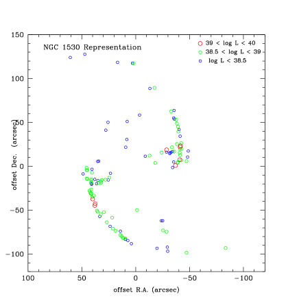
Figure 2: Representation of the position and luminosities of the catalogued H ii regions of NGC 1530. The coordinates of the centre of the image are R.A.=$4^{\rm h}\,23^{\rm m}\,26.7^{\rm s}$ and DEC=75^∘ 17^′ 44^′′ (J2000). The ionized regions around the nucleus of the galaxy have not been included in the catalogue, as their mutual proximity makes it difficult to delineate them accurately.

2.3 Fabry–Pérot observations

While the photometry from the narrow–band observations gives us a measurement of the H$\alpha$ luminosity for each H ii region in the galaxy and an estimate of its area, kinematic information can be obtained with Fabry-Pérot interferometry. The three barred galaxies, NGC 3359, NGC 6951 and NGC 1530 were observed with the TAURUS-II Fabry-Pérot interferometer at the 4.2m William Herschel Telescope (WHT) on La Palma. The data reduction for each galaxy is explained respectively in Rozas et al. (2000b) for NGC 3359, in Rozas et al. (2002) for NGC 6951 and in Zurita et al. (2004) for NGC 1530, and the observational parameters are shown in Table 1.

The observations consist of exposures at a set of equally stepped separations of the etalon, allowing us to scan the full wavelength range of the H$\alpha$ emission line in the galaxy. For the three galaxies, the observed emission wavelengths were scanned in 55 steps with exposures times at each position of the etalon of 140s for NGC 3359 and NGC 6951, and 150s for NGC 1530. An appropriate redshifted narrow–band H$\alpha$ filter is used as an order–sorting filter. Wavelength and phase calibration were performed using observations of a calibration lamp before and after the exposure of the data cube. The final calibrated data cube has three axes, $x$ and $y$, corresponding to the spatial coordinates in the field, and $z$, which corresponds to the wavelength direction. The free spectral ranges for each galaxy are 17.22Å for NGC 3359 and NGC 6951 and 18.03Å for NGC 1530, with a wavelength interval between consecutive planes of 0.34Å for NGC 3359 and NGC 6951 and 0.41Å for NGC 1530. These values give a finesse of 21.5 for NGC 3359 and NGC 6951 and 21.2 for NGC 1530, so that our 55 planes imply a very slight oversampling. We checked that there is no contamination of the atmospheric OH lines in our observations.

The continuum of the observational data cube was determined by fitting a linear relation to the line–free channels, and was then subtracted from the line emission channels. From the continuum subtracted data cube we can obtain a detailed description of the spatial distribution of intensities and velocities provided by the moment maps: the total intensity (zeroth moment), velocity (first moment) and velocity dispersion (second moment) maps. The general procedure for obtaining the moment maps is explained in Knapen (1997). The intensity map is used to identify each H ii region in the catalogue with the equivalent H ii region in the data cube, as we explain in the next section.

3 Relating the photometric and spectroscopic data sets

In order to assign the H$\alpha$ luminosity of each H ii region to its corresponding line profile, we need to identify each H ii region in the Fabry-Pérot data cube with its corresponding region in the continuum subtracted H$\alpha$ flux calibration image (Fig. 1 for NGC 1530). There are some problems involving the identification of the H ii regions:

• The pixel scales of the CCDs used in the photometric observations and those used in the observations with the Fabry–Pérot interferometer are not the same (see Table 1). Thus, a region in the calibration image will be scaled differently from the intensity map extracted from the data cube.

• Not all of the H ii regions in the catalogue derived from the calibration image appear in the intensity map, which is used to select the aperture for the extraction of the line profiles in the continuum subtracted data cube. This is because the total exposure time for each plane in the data cube is shorter than the exposure time for the H$\alpha$ image and the Fabry–Pérot throughput is less than that of the direct imaging cameras.

With these considerations in mind the identification of each H ii region was made interactively on the computer screen. Once we recognized a given catalogued H ii region in the intensity map we fitted a two-dimensional Gaussian function to the emission feature and obtained the centre for the H ii region in the intensity map. With this procedure we obtain a file containing, for each H ii region detected in the Fabry–Pérot observations, its coordinates in pixels, and its luminosity and radius assigned in the catalogue. In this way, we assign an integrated H$\alpha$ flux to the H ii region spectrum obtained from the data cube and relate the photometric data with the kinematic information extracted from the interferometric observations. The following notes for each galaxy clarify the procedure for the identification of the H ii regions:

• NGC 1530: As shown in Table 1, the pixel scales for the calibration image and the intensity map are similar, so that most of the H ii regions are quite easily identified in both the calibration image and the intensity map of the Fabry–Pérot. However, there are some catalogued H ii regions which appear with only a faint signal in the data cube. These H ii regions are too faint to be detected as an H ii region feature in the intensity map, only those which are isolated could be identified. Although we could not fit a centre to these features in the intensity map, we could extract the line profile of the faint emission zone because the continuum subtracted data cube contained sufficient signal. In these cases a valid H ii region spectrum could be extracted and analyzed, but in the remaining faint regions this was not possible. Besides, the projected CCD size for the intensity map was too small to cover the whole of the spiral arms, so that some H ii regions at the ends of both spiral arms which are catalogued in the calibrated image do not appear in the intensity map and could not be identified.

  There are a few cases in which a single emission zone in the intensity map corresponds to more than one H ii region in the catalogue. We have found 6 faint emission zones in which this situation appears. For these cases the spectrum of the central component was assigned to the most luminous H ii region inside the emission zone. Of the 119 H ii regions which form the catalogue of NGC 1530, 98 could be reliaby identified in the Fabry-Pérot data, the remainder belonging to one of the categories described above.

• NGC 3359: Apart from 20 H ii regions that are outside the field of the intensity map the rest of the 202 H ii regions down to a value of log L${}_{\scriptsize{\mbox{H}}\alpha}=37.7$ ( erg s^-1) could be easily identified in the data cube. This exact lower limit of identification is somewhat arbitrary. Although the lower limits to the luminosity of the detected H ii regions in the calibration image is log L${}_{\scriptsize{\mbox{H}}\alpha}=36.70$ ( erg s^-1), the line profiles extracted for H ii regions with an H$\alpha$ luminosity below log L${}_{\scriptsize{\mbox{H}}\alpha}=37.7$ ( erg s^-1) have velocity dispersions with large errors (see Table 5). Besides, the present study is confined to the most luminous H ii regions for each galaxy, so we consider that the information from the faintest H ii regions in the study of the log L${}_{\scriptsize{\mbox{H}}\alpha}$–log $\rm\sigma_{nt}$ diagrams is of limited value and importance in this context.

• NGC 6951: Down to a limit of log L${}_{\scriptsize{\mbox{H}}\alpha}=38.0$ ( erg s^-1), there are 91 H ii regions catalogued and we could identify 73 in the intensity map. We have found 7 cases in which more than one H ii region corresponds to a single emission zone in the intensity map. This is due to the large difference in pixel scales between the intensity map and the H$\alpha$ calibration image (0.28^′′/pix, for the photometric data and 0.58^′′/pix for the Fabry–Pérot observations, see Table 1). We considered in detail only 4 of these cases (regions 4, 5, 17, and 26 in the catalogue); the other 3 were discarded because they are small, faint regions having more than two catalogued H ii regions inside the emission feature. In the 4 H ii regions 4, 5, 17, and 26 more intense knots could be identified inside the emission zones related to the H ii regions catalogued and the line profiles were extracted for these knots.

  Taking into account the problems involved in the identification of the H ii regions in the three galaxies described above, we finally used data from 98 regions in NGC 1530, 202 in NGC 3359 and 73 in NGC 6951.

4 Extraction of the line profiles

Once we have identified the H ii regions for each galaxy in each corresponding intensity map, we obtained the integrated spectrum of each one from the continuum subtracted H$\alpha$ data cube. The selection of the aperture that defines the integrated spectrum for the H ii regions requires special attention. In the case of an isolated H ii region the radius defined in the catalogue gives us an idea of the radius for the best aperture. But in the case of a non-isolated H ii region or a region that is not spherical (especially those located along the bar), the radius is taken here as a reference value to identify and separate it from its neighbours.

The error in the velocity dispersion of the most intense, central, component when different apertures are chosen to extract the line profile, is shown in Table 2. In this table we have selected as conservative examples, three non-isolated H ii regions from each galaxy of our sample. We extracted their line profiles for different apertures: two rectangular apertures with different sizes, one bigger than the other, and a circular aperture. The apertures are specified in Table 2, the radius for the circular aperture is the mean value of the radii obtained from the rectangular apertures, assuming their areas are equal to those of circular projected areas.

As shown in this table, the velocity dispersion of the central, most intense, component obtained using different apertures does not change significantly and the changes are within the error bars of $\sigma$. The errors in velocity dispersion shown here are those given by the fit program when a least squares fit is applied to the observed function using the proposed function formed by Gaussian components. For all the H ii regions listed in Table 2, the variation in $\sigma$ obtained with the different selected apertures is comparable with the estimate given by the fitting program. In two cases (regions 11 and 35) these variations are significantly larger than the rest. The cause is somewhat different for the two cases. For region 11 there are two strong peaks (one significantly stronger than the other), which leads to a larger error in $\sigma$; for region 35, which is the faintest chosen region in NGC 1530, the error is larger due to an inferior S:N ratio. The examples shown in Table 2 give us some freedom to take the aperture that we think can best specify the H ii region, which can be hard to judge when the H ii regions are crowded. For simplicity, we chose rectangular apertures and extracted the integrated profiles with the task profil in the GIPSY package.

The selected regions taken as examples in Table 2 are not isolated but embeded in crowded fields of H ii regions, so the results in Table 2 give estimates of the upper limit to the uncertainty in the velocity dispersion for the central component when using different apertures. For isolated H ii regions the uncertainties will be lower because there is no contamination by emission from neighbouring regions. In these cases the aperture is taken to include all the emission defined in the intensity map.

Table 2: Estimates of the uncertainties in the velocity dispersion due to changes in aperture dimensions for the central and most intense Gaussian function fitted to the observed spectrum for a group of selected H ii regions in the barred galaxies: NGC 3359, NGC 1530 and NGC 6951. The catalogued radii of the H ii regions (Rad. in column 3) and the apertures are in pixels in the intensity maps and $\sigma$ in  km s^-1. The third value for $\sigma$ is obtained with a circular aperture of radius r. This radius r is the mean value of the radii obtained from the rectangular apertures, assuming their areas are equal to those of circular projected areas.

Region	log L${}_{\scriptsize{\mbox{H}}\alpha}$	Rad.	$\sigma$	Aperture	$\sigma$	Aperture	$\sigma$	r
(galaxy)	( erg s-1)	(pix)	( km s-1)	(pix$\times$pix)	( km s-1)	(pix$\times$pix)	( km s-1)	(pix)
11(N1530)	39.4338	6.0	39.5$\pm$5.0	15$\times$8	38.6$\pm$4.0	7$\times$5	41.5$\pm$4.3	4.8
15(N1530)	39.3467	5.9	40.7$\pm$0.7	7$\times$7	41.0$\pm$0.6	6$\times$4	40.4$\pm$0.6	3.4
35(N1530)	38.8842	3.8	35.3$\pm$5.1	7$\times$8	34.6$\pm$3.3	6$\times$4	38.8$\pm$3.8	3.5
63(N3359)	38.4188	5.9	26.0$\pm$0.9	7$\times$5	25.2$\pm$0.8	4$\times$5	25.4$\pm$0.8	3.3
51(N3359)	38.5170	5.1	27.1$\pm$0.8	8$\times$6	25.6$\pm$0.8	6$\times$5	26.7$\pm$0.9	3.5
41(N3359)	38.5965	6.1	28.4$\pm$0.5	8$\times$11	28.3$\pm$0.5	7$\times$6	28.7$\pm$0.5	4.5
21(N6951)	38.5823	2.9	31.0$\pm$0.8	7$\times$8	31.1$\pm$0.7	5$\times$5	31.2$\pm$0.6	3.5
28(N6951)	38.4441	2.6	24.8$\pm$0.8	8$\times$6	24.7$\pm$0.7	4$\times$5	24.8$\pm$0.6	3.2
3(N6951)	39.1203	4.4	29.1$\pm$0.5	7$\times$8	28.7$\pm$0.5	6$\times$5	28.9$\pm$0.4	3.6

5 Spectral analysis

For each H ii region, the line profile was extracted taking an integration of the selected zone in each plane of the continuum subtracted data cube. The number of Gaussians for each decomposition was given by the requirements of the fit program in each line profile. The fits were performed with the task profit in the GIPSY program, which lets us to fit for each spectrum up to five Gaussian components. In Fig. 3 we show some integrated line profiles fitted with the optimized number of Gaussians.

Although, the decomposition of the spectra into Gaussian functions is quite clear for most of the line profiles, there is a minority of cases in which the number of Gaussians required to fit the spectrum can be ambiguous. We treated these cases carefully for each galaxy.

Figure 3: Integrated line profiles for four H ii regions of the three galaxies: NGC 1530, NGC 3359 and NGC 6951. The spectral resolutions in the line profiles are 18.6  km s^-1 for NGC 1530, and 15.6  km s^-1 for NGC 3359 and NGC 6951.

In NGC 3359 there are 21 spectra (11.5% of the total number of identified H ii regions) that have single isolated wavelength points with high intensity values located near the central component. To check the possible effect of these on the line widths of the central components, we fitted these spectra with a single and with two Gaussian components. In just 6 cases the values of the velocity dispersion of the principal component for the line profiles fitted with one or with more Gaussians do not coincide within the error bars, but the differences are really small. In addition, NGC 3359 has 7 (3.8%) regions whose line profiles show low intensity components which are not clearly defined. Except for 2 cases the velocity dispersion of the single Gaussian fitted to the spectrum coincides within the error bars with the values of the velocity dispersion of the central peak when the spectrum is fitted with more than one Gaussian, and the differences even in these 2 cases are negligible. In NGC 6951 there are 6 (8.2%) ambiguous fits and in all of them the velocity dispersions associated with the central peak coincide for the two possible fits within the error bars. In NGC 1530 we do not find ambiguous line profiles, because of the high S:N ratio of its line profiles.

These apparent ambiguities give an idea of the quality of the fit; those line profiles which do not have clear multiple Gaussian components give values of the velocity dispersion for the central peak which do not differ significantly when a single or multiple Gaussian fit is applied, because the subsidiary peaks are fairly weak, and well shifted in wavelength from the line centre.

5.1 Statistics of the number of Gaussian components fitted to each spectrum

In Table 3 we list, for each galaxy, the fraction of the line profiles with different Gaussian decompositions. Most of the line profiles ($\sim$70%) have two or three Gaussian components. This result is similar to that found by Arsenault & Roy (1996) for 47 giant extragalactic H ii regions in 26 nearby galaxies. They found that 43% of the spectra had profiles characterized by a Voigt profile and 21% were fitted with two Gaussians. The Voigt profile would correspond better in our case to three Gaussian components, a central peak and two symmetric low intensity Gaussians.

Table 3: Spectral Gaussian decomposition frequency analysis for the integrated line profiles extracted for the identified H ii regions in NGC 1530, NGC 3359 and NGC 6951. Each column shows the fraction of the total emission profiles which are fitted by the specified number of Gaussian components (GC).

Galaxies	1 GC	2 GC	3 GC	4 GC	5 GC
NGC 1530	10.2%	21.4%	50.0%	18.4%	1.0%
NGC 3359	26.9%	47.3%	24.7%	1.0%	–
NGC 6951	25.0%	45.0%	26.0%	4.0%	–

Although we will not attempt in this paper to find a physical explanation for all the secondary components that appear in the line profiles, it is interesting to note that most of the line profiles are characterized by a central peak and one or two high velocity features, and just a small fraction contain two central peaks of comparable amplitude. In order to show this statement we have classified the integrated spectra for all the identified H ii regions in a qualitative form. The results are shown in Table 4. When there is a single Gaussian, this component describes the peak of the line profile. Secondary Gaussian components located at more than $\sim$ 35  km s^-1 from the centre of the more intense Gaussian are taken to be wing features. For example, a spectrum can have two Gaussians describing the central peak (2 P) or three components, one describing the central peak and the others classified as wing features (1 P+2 W). It is interesting to note that there is a relation between the fraction of the multiple component Gaussians in the central peak and the inclination of the galaxy. The inclinations of the galaxies are 55^∘, 53^∘and 42^∘, for NGC 1530, NGC 3359 and NGC 6951. The most inclined galaxy has the biggest fraction of line profiles classified as 2 P. This means that there is a crowding effect in the H ii region line profiles which grows principally with increasing inclination.

Table 4: Frequency distribution of the component decomposition for the integrated line profiles extracted for the selected H ii regions in NGC 1530, NGC 3359 and NGC 6951. P; central peak or component included in the central peak, W; high velocity low intensity wing feature.

	1 P	1 P+1 W	1 P+2 W	2 P	2 P+1 W	2 P+2 W	2 P+3 W
NGC 1530	9.2%	8.2%	30.5%	14.3%	18.4%	18.4%	1.0%
NGC 3359	28.0%	35.7%	18.1%	12.1%	5.0%	1.1%	–
NGC 6951	25.0%	41.0%	27.0%	3.0%	–	4.0%	–

6 The luminosity v. non–thermal velocity dispersion relation

6.1 Construction of the diagrams

From the integrated spectra of the identified H ii regions in the three galaxies NGC 3359, NGC 6951 and NGC 1530, we have selected the widths of the most intense Gaussian components. These observed widths were corrected for the natural, thermal and instrumental line widths. The non–thermal velocity dispersion was obtained from the following expression:

$$\sigma_{\rm nt}=((\sigma_{\rm obs})^{2}-(\sigma_{\rm n})^{2}-(\sigma_{\rm t})^{2}-(\sigma_{\rm inst})^{2})^{1/2}$$ (1)

where $\sigma_{\rm obs}$, $\sigma_{\rm n}$, $\sigma_{\rm t}$ and $\sigma_{\rm inst}$ are the observed, natural, thermal and instrumental widths, respectively. The natural width has a value of 3  km s^-1 (O’Dell & Townsley 1988). The thermal width was taken assuming a constant temperature inside the H ii region of $10^{4}$ K, which corresponds to 9.1  km s^-1(Osterbrock 1989). The instrumental width for each galaxy was obtained from the data cube taken with the calibration lamp. We extracted a line profile from this calibration data cube centred on the optical centre of the instrument, where the line profile of best S:N was obtained. The instrumental width is the half-width, $\sigma$, of the single Gaussian component fitted to the instrumental line profile. The values we found for each observation are (17.4$\pm$0.4)  km s^-1, (16.3$\pm$0.3)  km s^-1and (15.9$\pm$0.3)  km s^-1for NGC 1530, NGC 3359 and NGC 6951, respectively. The instrumental line profile was analyzed, extracting line profiles with different apertures at different distances from the optical centre of the instrument; differences in the instrumental widths were no larger than  10% across the field of view.

In order to construct the log L${}_{\scriptsize{\mbox{H}}\alpha}$–log $\rm\sigma_{nt}$ diagram, we need to find the luminosity associated with the central most intense component of the integrated spectrum. In the case where the line profile is fitted by a single Gaussian the assignment is straightforward, but when the line profile is fitted with more components there is an uncertainty in the assignment of the luminosity. This is because the luminosity of the catalogue corresponds to the integrated luminosity of the H ii region identified with the REGION program, while when a line profile is fitted by more than a single Gaussian, it is the sum over the areas of all the components which represents the integrated luminosity given by the catalogue.

To cope with this problem, we have treated specially the H ii regions with two clearly defined central peaks and with the most intense one having less than 80% of the total area below the fitted Gaussians. To these H ii regions we assigned the fraction of the luminosity of the H ii region in the catalogue corresponding to the fractional integrated intensity of the strongest Gaussian, while to the other regions we assigned the full value of the catalogue luminosity.

In Fig. 4a we show the logarithmic H$\alpha$ luminosity of the H ii regions in the three galaxies versus the logarithmic non–thermal velocity dispersion of the central most intense component of their integrated spectra. In Fig. 4b we show the same distribution but, where appropiate, using the fractional H$\alpha$ luminosity corresponding to the central peak, as explained above.

The diagrams show that the range of non–thermal velocity dispersions at a given luminosity decreases with increasing luminosity of the H ii region, i.e. the diagram becomes narrower for higher luminosities. In both Figs. 4a and 4b it is easy to see that there is an observed upper limit in log L${}_{\scriptsize{\mbox{H}}\alpha}$, i.e. for a given $\rm\sigma_{nt}$; there is an observed upper limit in log L${}_{\scriptsize{\mbox{H}}\alpha}$ where no H ii regions with lower velocity dispersion are found.

It is interesting to note the ranges of uncertainty in the non–thermal velocity dispersion of the H ii regions in these diagrams. The uncertainties are the error bars in $\sigma_{\rm nt}$ given by the fit procedure and are related to the signal to noise ratio of the line profiles. We have divided the diagrams into two zones, separated by a value of the non–thermal velocity dispersion of 13  km s^-1, a canonical estimate of the sound speed in the interestellar medium. The relative errors in velocity dispersion for H ii regions with $\rm\sigma_{nt}<13$  km s^-1are $\sim$28%, while for H ii regions with $\rm\sigma_{nt}>13$  km s^-1the relative errors are $\sim$4%, as shown in Table 5. The difference in the mean relative errors is because for $\rm\sigma_{nt}<13$  km s^-1, the observed line width is approaching the resolution of the instrument, and the S:N is also falling because the regions have lower luminosity.

Table 5: Fraction (in %) of the number of H ii regions for each galaxy with $\rm\sigma_{nt}<13$  km s^-1and $\rm\sigma_{nt}>13$  km s^-1and the mean value of the relative errors in the velocity dispersion of the central components for these two groups of H ii regions.

	H ii regions with $\rm\sigma_{nt}>13$  km s-1		H ii regions with $\rm\sigma_{nt}<13$  km s-1
Galaxy	Fraction	$\Delta\rm\sigma_{nt}$	Fraction	$\Delta\rm\sigma_{nt}$
NGC 1530	88.2%	4.1%	11.8%	32.1%
NGC 3359	54.4%	4.6%	45.6%	24.9%
NGC 6951	48.4%	3.8%	51.6%	27.8%

Figure 4: log L${}_{\scriptsize{\mbox{H}}\alpha}$–log $\rm\sigma_{nt}$ diagram for the H ii regions in NGC 1530, NGC 3359, and NGC 6951. In a. the H$\alpha$ luminosity of the H ii region is the luminosity given by the catalogue, while in b. the H$\alpha$ luminosity is the fraction of the H$\alpha$ luminosity from the catalogue corresponding to the fractional integrated intensity of the strongest Gaussian component in the H ii region spectrum. $\rm\sigma_{nt}$ is the non–thermal velocity dispersion corresponding to the most intense central component.

6.2 Envelope of the log L${}_{\scriptsize{\mbox{H}}\alpha}$–log $\rm\sigma_{nt}$ diagram

We have devised an automatic method to find an envelope for the Figs. 4a and 4b. Starting at a certain logarithmic H$\alpha$ luminosity and increasing it in bins of fixed widths in logarithm of luminosity, we selected for each bin the H ii region with the lowest value of the non–thermal velocity dispersion. Changing the starting point in luminosity and the bin widths we optimized the envelope that best defines the log L${}_{\scriptsize{\mbox{H}}\alpha}$–log $\rm\sigma_{nt}$ distribution. The points which best define the envelopes in the log L${}_{\scriptsize{\mbox{H}}\alpha}$–log $\rm\sigma_{nt}$ diagrams for each galaxy and the distributions taking into account all the galaxies are shown in Figs. 5a and 5b. Although the lower limits in logarithmic H$\alpha$ luminosity change from one galaxy to another, the bin widths that best define the envelope take the same value of 0.15 in all the distributions (see Tables 7 and 8).

Figure 5: log L${}_{\scriptsize{\mbox{H}}\alpha}$–log $\rm\sigma_{nt}$ diagram for the H ii regions in NGC 1530, NGC 3359 and NGC 6951 and the corresponding points defining the best envelopes for each galaxy. Also shown is the representative linear fit to the envelope for each galaxy. The points marked with a cross represent the envelope when the H ii regions of the three galaxies are considered as a single log L${}_{\scriptsize{\mbox{H}}\alpha}$–log $\rm\sigma_{nt}$ distribution. a. the luminosity of the H ii region is that obtained from the catalogue, b. the H$\alpha$ luminosity of the H ii region is a fraction of the luminosity from the catalogue, corresponding to the most intense Gaussian peak in the emission line profile.

The best way of fitting the points on the envelope must take into account the uncertainties in the logarithmic H$\alpha$ luminosity of the H ii regions and in the velocity dispersion of the line profiles. Except for 4 H ii regions on the envelope defined by NGC 6951, the rest of the regions on the envelopes have luminosities above ${\rm log\leavevmode\nobreak\ L_{\scriptsize{\mbox{H}}\alpha}}>38.5$ ( erg s^-1). The uncertainties in H$\alpha$ luminosity for H ii regions with a ${\rm log\leavevmode\nobreak\ L_{\scriptsize{\mbox{H}}\alpha}}>38.5$ ( erg s^-1) is less than 10% for NGC 3359, $\sim$10% for NGC 6951 and $\sim$20% for NGC 1530. The high value for the uncertainty in luminosity for the H ii regions in NGC 1530 is because this galaxy is further away than the others and the image was taken with the JKT (1m Telescope); H ii regions with the same H$\alpha$ luminosity but located at greater distance will be seen with lower S:N ratio. The uncertainty in the velocity dispersion is obtained from the estimated error given by the fit program in decomposing the line profiles.

In order to obtain simultaneously both uncertainties we use a linear fit which gives a weight, w, to each point of the envelope defined by:

$${\rm w}=((\Delta{\rm log\leavevmode\nobreak\ L_{\scriptsize{\mbox{H}}\alpha}})^{2}+(\Delta{\rm log\leavevmode\nobreak\ \rm\sigma_{nt}})^{2})^{-1/2}$$ (2)

where $\Delta{\rm log\leavevmode\nobreak\ L_{\scriptsize{\mbox{H}}\alpha}}$ and $\Delta{\rm log\leavevmode\nobreak\ \rm\sigma_{nt}}$ are the relative errors in logarithmic H$\alpha$ luminosity and logarithmic $\rm\sigma_{nt}$.

We have taken into account the influence of the selected bin width and the logarithmic H$\alpha$ luminosity starting point on the definition of the envelope, and specially on the slope of the envelope. In Table 6, we show the slopes for different selected bin widths. The values of the slopes are the median values of the slopes for the different starting points in the range of logarithmic H$\alpha$ luminosity, and the corresponding errors are the standard deviations for all the slopes for different starting points. As can be seen from this table, a change in the bin width or in the starting point does not affect significantly the values of the slopes, which means that the procedure we have used is robust against these changes.

Table 6: Variation of the log L${}_{\scriptsize{\mbox{H}}\alpha}$-log $\rm\sigma_{nt}$ envelope slope with the selected bin width. Each value and its error correspond respectively, to the median and standard deviation of the slopes for different bin starting points in log L${}_{\scriptsize{\mbox{H}}\alpha}$.

bin width	NGC 1530		NGC 6951		NGC 3359
dex	frac of L${}_{\scriptsize{\mbox{H}}\alpha}$	total L${}_{\scriptsize{\mbox{H}}\alpha}$	frac of L${}_{\scriptsize{\mbox{H}}\alpha}$	total L${}_{\scriptsize{\mbox{H}}\alpha}$	frac of L${}_{\scriptsize{\mbox{H}}\alpha}$	total L${}_{\scriptsize{\mbox{H}}\alpha}$
0.10	$2.4\pm 0.2$	$1.9\pm 0.3$	$0.8\pm 0.2$	$0.8\pm 0.2$	$1.6\pm 0.3$	$1.1\pm 0.3$
0.15	$2.4\pm 0.2$	$2.0\pm 0.2$	$1.2\pm 0.4$	$1.2\pm 0.4$	$1.5\pm 0.2$	$1.4\pm 0.3$
0.20	$2.4\pm 0.2$	$1.9\pm 0.1$	$1.6\pm 1.9$	$1.6\pm 1.9$	$1.6\pm 0.2$	$1.4\pm 0.3$

Finally, we have selected as the representative fit to the envelope of each distribution that found from the variation of the starting point with a selected bin of 0.15, for which the envelopes are best defined. The $y$ coordinate of the zero point and the slope for each representative linear fit are the median values of the corresponding quantities, taken as the starting point in luminosity is varied. The results are shown in Tables 7 and 8 and plotted in Figs. 5a and 5b.

From Tables 7 and 8 and the corresponding Figs. 5a and 5b, we can see that the envelope in the log L${}_{\scriptsize{\mbox{H}}\alpha}$–log $\rm\sigma_{nt}$ distribution is not particularly well defined. The envelopes for each galaxy have slopes with similar values but the errors in the fits are large. In any case, the results of the linear fits for each galaxy agree broadly with the result of Arsenault et al. (1990). These authors found a limit in the upper boundary of ${\rm log\leavevmode\nobreak\ F_{\scriptsize{\mbox{H}}\alpha}}<(2.18\leavevmode\nobreak\ {\rm log\leavevmode\nobreak\ \rm\sigma_{nt}}-16.15)$ in the plane H$\alpha$ surface brightness - non–thermal velocity dispersion for the H ii regions they detected in NGC 4321.

Table 7: Representative fits to the envelopes of the log L${}_{\scriptsize{\mbox{H}}\alpha}$–log $\rm\sigma_{nt}$ distributions for NGC 1530, NGC 3359 and NGC 6951 and for the distribution defined with all the H ii regions in the three galaxies. The logarithmic H$\alpha$ luminosity corresponds to the value given in the calibration catalogue.

	Bin	Envelope fit
NGC 1530	0.15	log L${}_{\scriptsize{\mbox{H}}\alpha}$$\sim$(37.0$\pm$0.3)+(2.0$\pm$0.2) log $\rm\sigma_{nt}$
NGC 3359	0.15	log L${}_{\scriptsize{\mbox{H}}\alpha}$$\sim$(37.5$\pm$0.4)+(1.4$\pm$0.7) log $\rm\sigma_{nt}$
NGC 6951	0.15	log L${}_{\scriptsize{\mbox{H}}\alpha}$$\sim$(37.7$\pm$0.4)+(1.2$\pm$0.4) log $\rm\sigma_{nt}$
All galaxies	0.15	log L${}_{\scriptsize{\mbox{H}}\alpha}$$\sim$(37.4$\pm$0.2)+(1.78$\pm$0.14) log $\rm\sigma_{nt}$

Table 8: The same parameters as shown in Table 7, but the logarithmic H$\alpha$ luminosity is given by the fraction of the logarithmic H$\alpha$ luminosity of the catalogue corresponding to the most intense Gaussian peak.

	Bin	Envelope fit
NGC 1530	0.15	log L${}_{\scriptsize{\mbox{H}}\alpha}$$\sim$(36.1$\pm$0.2)+(2.4$\pm$0.2) log $\rm\sigma_{nt}$
NGC 3359	0.15	log L${}_{\scriptsize{\mbox{H}}\alpha}$$\sim$(37.4$\pm$0.2)+(1.5$\pm$0.7) log $\rm\sigma_{nt}$
NGC 6951	0.15	log L${}_{\scriptsize{\mbox{H}}\alpha}$$\sim$(37.7$\pm$0.4)+(1.2$\pm$0.4) log $\rm\sigma_{nt}$
All galaxies	0.15	log L${}_{\scriptsize{\mbox{H}}\alpha}$$\sim$(37.5$\pm$0.1)+(1.57$\pm$0.07) log $\rm\sigma_{nt}$

6.2.1 Envelope for the best determined velocity dispersion

In order to find better defined envelopes than those shown in Figs. 5a and 5b and minimize the errors in the slopes of the envelopes, we have eliminated the H ii regions in the log L${}_{\scriptsize{\mbox{H}}\alpha}$–log $\rm\sigma_{nt}$ diagram which have large errors in their velocity dispersions. From Table 5 we see that the regions with $\rm\sigma_{nt}<13$  km s^-1 have relative errors of $\sim$28%, so we have eliminated them from the log L${}_{\scriptsize{\mbox{H}}\alpha}$–log $\rm\sigma_{nt}$ diagram and extracted again the envelope for all the galaxies.

The results are shown in Figs. 6 and 7. More clearly defined envelopes are defined for the H ii regions with $\rm\sigma_{nt}>13$  km s^-1, for both distributions: when the total logarithmic H$\alpha$ luminosity from the catalogue is considered and when an appropiate fraction is used for those H ii regions with the central peak defined by two Gaussian components of comparable intensities. The linear fit for the envelope is ${\rm log\leavevmode\nobreak\ L_{\scriptsize{\mbox{H}}\alpha}}=(36.8\pm 0.7)+(2.0\pm 0.5)\leavevmode\nobreak\ {\rm log\leavevmode\nobreak\ \rm\sigma_{nt}}$ in the case where the logarithmic H$\alpha$ luminosity of the H ii region is given by the catalogue (Fig. 6). For the case where the logarithmic H$\alpha$ luminosity is a fraction of the H ii region luminosity, the linear fit is ${\rm log\leavevmode\nobreak\ L_{\scriptsize{\mbox{H}}\alpha}}=(36.8\pm 0.6)+(2.0\pm 0.5)\leavevmode\nobreak\ {\rm log\leavevmode\nobreak\ \rm\sigma_{nt}}$ (see Fig. 7).

Although the results found here do not agree with the L–$\sigma$ relation proposed by Terlevich & Melnick (1981), they do agree quite well with those found by Arsenault et al. (1990) for the H ii regions with the highest surface brightness in NGC 4321. They found that these regions can be fitted by ${\rm log\leavevmode\nobreak\ F}_{\scriptsize{\mbox{H}}\alpha}=(2.57\pm 0.49)\leavevmode\nobreak\ {\rm log\leavevmode\nobreak\ \rm\sigma_{nt}}-(17.21\pm 0.39)$, where ${\rm log\leavevmode\nobreak\ F}_{\scriptsize{\mbox{H}}\alpha}$ is the surface brightness of the H ii region. Rozas et al. (1998) found a linear fit to the H ii regions on the envelope of ${\rm log\leavevmode\nobreak\ L_{\scriptsize{\mbox{H}}\alpha}}=36.15+2.6\leavevmode\nobreak\ {\rm log\leavevmode\nobreak\ \rm\sigma_{nt}}$ for the H ii regions in NGC 4321 with central component widths above 10  km s^-1, and this linear fit is in fair agreement with those shown in Tables 7 and 8 and also with the linear fits obtained for H ii regions with $\rm\sigma_{nt}>13$  km s^-1.

Finally, it is also interesting to note that the slopes of the envelopes for both log L${}_{\scriptsize{\mbox{H}}\alpha}$–log $\rm\sigma_{nt}$ diagrams obtained by taking the luminosity of an H ii region directly from the catalogue, and the diagram taking the logarithmic H$\alpha$ luminosity of the region as a fraction of the catalogued luminosity, are the same. However, the log L${}_{\scriptsize{\mbox{H}}\alpha}$–log $\rm\sigma_{nt}$ diagram taking into account the fraction of the logarithmic H$\alpha$ luminosity gives an envelope with less dispersion in its defining points.

Figure 6: log L${}_{\scriptsize{\mbox{H}}\alpha}$–log $\rm\sigma_{nt}$ diagram for the three galaxies with H ii regions having $\rm\sigma_{nt}>13$  km s^-1. The continous line represents the linear fit to the points on the envelope (bolder points in the diagram). The logarithmic H$\alpha$ luminosities are those in the photometric H ii region catalogue.

Figure 7: log L${}_{\scriptsize{\mbox{H}}\alpha}$–log $\rm\sigma_{nt}$ diagram for the three galaxies with H ii regions having $\rm\sigma_{nt}>13$  km s^-1 as in Fig. 6, but the logarithmic H$\alpha$ luminosities of the H ii regions are found as a fraction of the logarithmic H$\alpha$ luminosity from the catalogue, as explained in text. The envelope fit is somewhat tighter than that in Fig. 6, but the slope is the same.

6.2.2 Testing for metallicity dependence

The metallicity could affect the log L${}_{\scriptsize{\mbox{H}}\alpha}$-log $\rm\sigma_{nt}$ relationship as it affects the thermal velocity dispersion of a given region because the electron temperature of the H ii region depends on the metallicity and in this way the metallicity gradient across the disc of the spiral galaxies could be affecting the log L${}_{\scriptsize{\mbox{H}}\alpha}$–log $\rm\sigma_{nt}$ relation, as was first proposed by Terlevich & Melnick (1981). We check here this posibility.

We have assumed a constant electron temperature of $10^{4}$ K for all the H ii regions, which gives a thermal broadening of 9.1  km s^-1. Electron temperatures of 5000 K and 15000 K give thermal broadenings of 6.4  km s^-1and 11.1  km s^-1respectively. Assuming a typical observed velocity dispersion of $\sigma=(22.0\pm 2.0)$  km s^-1 and a $\sigma_{\rm inst}=(16.3\pm 0.3)$  km s^-1, the non–thermal velocity dispersions for different temperatures are $\sigma_{\rm nt}(\rm T=5000\leavevmode\nobreak\ K)=(13.0\pm 3.8)$  km s^-1, $\sigma_{\rm nt}(\rm T=10000\leavevmode\nobreak\ K)=(11.2\pm 4.3)$  km s^-1and $\sigma_{\rm nt}(\rm T=15000\leavevmode\nobreak\ K)=(9.3\pm 5.3)$  km s^-1. Thus, the assumption of a constant temperature of $10^{4}$ K for all the H ii regions is a very reasonable approximation and the effect on the non–thermal velocity dispersion for a reasonable spread on the temperatures will be inside the error bars.

A test for how the radial metallicity gradient might be affecting the log L${}_{\scriptsize{\mbox{H}}\alpha}$–log $\rm\sigma_{nt}$ relation is shown in Fig. 8, where we show the positions in the log L${}_{\scriptsize{\mbox{H}}\alpha}$–log $\rm\sigma_{nt}$ diagram of the H ii regions of each galaxy located in increasing ranges of galactocentric radius. We take the length of the major axis of the galaxy out to a a blue surface brightness level of 25 mag arcsec^-2, $\rm R_{25}$, as the radial unit. The values of $\rm R_{25}$ for each galaxy are taken from de Vaucouleurs et al. (1991). From Fig. 8 it can be seen that there is no trend of the H ii regions at a given galactocentric radius, which presumably all have essentially the same metallicity, to be concentrated in a certain zone of the log L${}_{\scriptsize{\mbox{H}}\alpha}$–log $\rm\sigma_{nt}$ diagram. There is no observed systematic trend of $\rm\sigma_{nt}$ with galactocentric radius for a given luminosity, so we can discount the importance of the metallicity in this context.

Figure 8: Plot of the H ii regions at different deprojected galactocentric radii in the log L${}_{\scriptsize{\mbox{H}}\alpha}$–log $\rm\sigma_{nt}$ diagram for the three galaxies NGC 1530, NGC 3359 and NGC 6951, showing that radial effects (and hence by implication, metallicity effects) are not affecting systematically the log L${}_{\scriptsize{\mbox{H}}\alpha}$–log $\rm\sigma_{nt}$ relation.

7 The masses of the H II regions in the log L${}_{\scriptsize{\mbox{H}}\alpha}$–log $\rm\sigma_{nt}$ diagram

7.1 Virial Mass

The virial mass is obtained from Eq. 3 resulting from the application of the virial theorem.

$$\rm M=\frac{\rm\sigma_{nt}^{2}R}{G}$$ (3)

where $G$ is the gravitational constant, R is a specified radius of the H ii region, and $\rm\sigma_{nt}$ is the non-thermal velocity dispersion of the line profile, which is taken to be a representative value of the velocity of the gas within the region.

A good estimate of the relevant radius is subject to uncertainties which in most cases do not allow us to obtain a fiducial value. In order to obtain the virial mass, we have taken an estimate of the radius which is half of the radius in the H ii region catalogues. This is consistent with the method of Arsenault et al. (1990), who take the radius containing 40% of the total flux of the H ii regions to characterize their sizes and extract the line profiles with an aperture having twice these characteristic values. They based this criterion on the study of McCall, Hill & English (1990), who show that the 40% isophote is a consistent measure of the H ii region size because it is independent of the detection threshold and the calibration. The virial mass computed in this way for the H ii regions on the envelope and a selection of regions well below the envelope in luminosity in the log L${}_{\scriptsize{\mbox{H}}\alpha}$–log $\rm\sigma_{nt}$ diagram is shown in Tables 9 and 10 respectively.

7.2 Mass of the H II region inferred from the H$\alpha$ luminosity

The mass of the gas within the region is obtained by integrating over the measured volume of the region and multiplying it by the mass of the hydrogen atom, thus:

$${\rm M_{reg}}=f\int\phi^{1/2}<{\rm N}_{\rm e}>_{\rm rms}{\rm m}_{\rm p}{\rm dV}$$ (4)

where f is a factor accounting for the fraction of the neutral mass inside the region, $\phi$ is the filling factor and ${\rm<N_{e}>_{rms}}$ is the root mean square (r.m.s) electron density. The factor $f$, accounting for the fraction of the neutral mass inside the region that cannot be detected by the H$\alpha$ observations, is estimated to take a value $\sim 10$ from models by Giammanco et al. (2004).

In that paper, a model has been proposed which gives a good account of the propagation of ionizing radiation in H ii regions making well defined assumptions about the structure of the regions, and using these to compare with their observed properties. One of its key results is that the major fraction of the gas in an H ii region (and this applies to regions of all sizes, though the largest regions may show a somewhat smaller effect than the smallest) will remain neutral due to the pronounced inhomogeneity which is a well attested feature of the density distribution. In the paper a range of estimates of the neutral mass fraction inside the H ii regions is quoted, with a canonical value of close to an order of magnitude.

The r.m.s. electron density, ${\rm<N_{e}>_{rms}=\sqrt{<N_{e}^{2}>}}$, can be estimated from the emission measure (EM) of the H ii region. The Emission Measure is defined as the square of the electron density integrated along the line of sight.

$${\rm EM=\int_{0}^{s}N_{e}^{2}ds\approx<N_{e}^{2}><s>}$$ (5)

where $\rm<s>$ is the average value of the line of sight length across the H ii region over the projected area of the region, (see Zurita 2001). The emission measure can be related to the surface brightness of the H ii region via the theoretical formula given by Spitzer (1978):

$${\rm{L_{\scriptsize{\mbox{H}}\alpha}\over\pi R^{2}}=h\nu_{\scriptsize{\mbox{H}}\alpha}\alpha_{\scriptsize{\mbox{H}}\alpha}^{eff}(H_{0},T){N_{p}\over N_{e}}2.46\times 10^{17}\times{\rm EM}}$$ (6)

where ${\rm\alpha_{\scriptsize{\mbox{H}}\alpha}^{eff}(H_{0},T)}$ is the effective recombination coefficient of the H$\alpha$ emission line, ${\rm h\nu_{\scriptsize{\mbox{H}}\alpha}}$ is the energy of an H$\alpha$ photon and R is the radius (in cm) of the H ii region. From the H$\alpha$ luminosity and the radius obtained from the catalogues we can obtain the EM using Eq. 6 and the ${\rm<N_{e}>_{rms}}$ using Eq. 5. Values for these quantities are shown in Tables 9 and 10.

The filling factor $\phi$ is defined to take into account inhomegeneities in the density of the H ii regions. The inhomogeneities are schematized as condensations of gas, with electron density ${\rm N_{e}}$ within the condensations, and with negligible electron density in the intervening volume. The filling factor can be computed using the expression (see Appendix D in Zurita (2001)):

$$\phi={\rm(\frac{<N_{e}>_{rms}}{N_{e}})^{2}}$$ (7)

The values of $\phi$ for a selected set of H ii regions are shown in Tables 9 and 10. We adopt the mean value of ${\rm N_{e}\sim 135}$  cm^-3 taken from measurements by Zaritsky (1994). With the values of ${\rm<N_{e}>_{rms}}$ and $\phi$, we obtain the total mass of the H ii region via Eq. 4; the results are shown in Tables 9 and 10.

7.2.1 Mass of the stellar content in the H ii region

The total mass of a star cluster can be obtained by integrating the initial mass function (IMF), which gives the number of stars formed at the same time in a given range mass, over the total range mass ${\rm(m_{low},m_{up})}$.

$${\rm M_{stellar}=\int_{m_{low}}^{m_{up}}m\Phi(m)dm}$$ (8)

where ${\rm\Phi(m)}$ is the IMF, normally assumed to be a power of m, ${\rm\Phi(m)=Am^{\alpha}}$, $\alpha=-2.35$ for the Salpeter IMF (Salpeter 1955) and A is a normalisation factor.

In order to estimate the mass of the stars within the H ii region, we need to know A, the mass, ${\rm m_{low}}$, of the lowest mass star and the mass, ${\rm m_{up}}$, of the highest mass star. The normalization factor A can be obtained from the estimate of the mass of the ionizing stars, as we can put a lower physical limit $\rm m_{l_{i}}$ on the mass of these stars which contribute significantly to the ionization of the H ii region. This is done in the following way.

The ionizing mass is calculated by integrating over the masses of the stars that contribute significantly to the ionizing radiation using:

$${\rm M_{ionizing}=\int_{m_{l_{i}}}^{m_{up}}Am^{-1.35}dm}$$ (9)

The H$\alpha$ luminosity gives an equivalent number of O5(V) stars and using the mass of an O5(V) spectral type star from Vacca et al. (1996), an estimate of the ionizing mass inside the H ii region can be obtained. The mass limits in Eq. 9 are found assuming that the most massive ionizing star is an O3(V) type star and that the sum of all the stars with spectral type O9(V) or later do not contribute more than 10% to the total ionizing flux. Thus, ${\rm m_{l_{i}}}=22.1\rm M_{\odot}$ and ${\rm m_{up}}=51.3\rm M_{\odot}$ from the values from Vacca et al. (1996) for the masses of spectral type stars O3(V) and O9(V) respectively.

Once the normalization factor is known, the mass for the stellar cluster is obtained by integrating Eq. 8. In Tables 9 and 10 we show the total masses for two groups of H ii regions. The integration limits are ${\rm(0.1M_{\odot},100M_{\odot})}$. Using this mass range gives an upper limit to the stellar cluster mass, since in a real cluster the curve should be less steep than the Salpeter function for masses less than $\rm 1M_{\odot}$ .

The mass of the stellar content obtained in this way is meant as an estimate which allows us to obtain an order of magnitude idea of the fraction of the H ii region mass that is in stellar form. The Salpeter IMF is not necessarily the most representative functional form to describe the stellar content of the cluster that produces an H ii region. Massey et al. (1989) obtained a slope for the IMF of $(-2.9\pm 0.3)$ in the 9-85 $\rm M_{\odot}$ range for NGC 346 in SMC, and Relaño et al. (2002) found a slope of $(-3.7\pm 0.4)$ in the 24-54.1 $\rm M_{\odot}$ range. In addition, the total ionizing stellar mass obtained from the observed H$\alpha$ luminosity of the H ii region does not take into account the escape fraction of luminosity in density bounded regions and the equivalent number of stars of spectral type O5(V) gives only an approximation to the total ionizing mass. In fact, the total mass obtained from the equivalent number of O5(V) stars in NGC 346 represents 60% of the mass for the stars from spectral types O3(V) to O9(V) (see Relaño et al. 2002).

These uncertainties do not allow us to find a very accurate value of the mass of the stars within an H ii region, but we can obtain a fair estimate of the fraction of the total H ii region mass in stellar form. Applying different mass limits in Eq. 8 gives a fraction of the total H ii region mass in stellar form of 0.17% and 0.44% for mass ranges ${\rm(1M_{\odot},100M_{\odot})}$ and ${\rm(0.1M_{\odot},100M_{\odot})}$, respectively. If the mass obtained from the equivalent number of O5(V) spectral type stars were 60% of the total mass for stars earlier than O9(V), as is the case for NGC 346, the total mass in stellar form would not be more than 1% of the H ii region mass. Moreover, even using a much steeper IMF, $\alpha=-3.7$ as found in NGC 346, and integrating over a mass range of ${\rm(1M_{\odot},100M_{\odot})}$ gives a fraction of only 4.7% of the region mass in stellar form. These estimates agree with the stellar mass content for NGC 604 given by Yang et al. (1996), who estimated a fraction of stellar mass content in the total mass of the region between 4% and 1%.

Using these considerations we can see that the mass of the stellar cluster represents a relatively small fraction of the H ii region mass and for this reason it may be neglected in the comparisons between the H ii region mass obtained from the H$\alpha$ luminosity and the virial mass.

7.3 Discussion

As can be seen from Tables 9 and 10, the virially estimated mass of the H ii regions located on the envelope is close to the total mass of the H ii region, the ratio M_vir/M_reg is between 1 and 4 (last column in Table 9). Virial masses for the H ii regions located well above the envelope in $\sigma_{\rm nt}$ are however bigger than their corresponding total H ii region masses, the ratios M_vir/M_reg range from 7 to 15 as shown in last column in Table 10. This result shows that the H ii regions located on the envelope may well be virialized systems or at least close to virial equilibrium, while the velocity dispersions from the H ii regions located well above the envelope in $\sigma_{\rm nt}$ in the log L${}_{\scriptsize{\mbox{H}}\alpha}$–log $\rm\sigma_{nt}$ diagram show the presence of other processes that affect the internal kinematics of the H ii regions.

The fact that the velocity dispersions of the principal velocity component can be affected by a number of processes has been investigated by Yang et al. (1996) for the nearby region NGC 604 in M33. They mapped this region with Fabry–Pérot interferometry and extracted line profiles for each pixel in the map. The velocity dispersion distribution for all the positional line profiles show that the numerous points with high intensities define a narrow band with a mean value of $\rm\sigma_{nt}\sim$12  km s^-1, and a lower limit of $\rm\sigma_{nt}\sim$9  km s^-1, while the few low intensity points have higher velocity dispersions. From comparison of the total mass of NGC 604 and the virial mass obtained from the underlying velocity dispersion values they conclude that gravitation may provide the basic mechanism for most positions, while other mechanisms are responsible of the excess broadening at the low intensity points. It is clear that these mechanisms affect even the H ii regions close to the envelope in Fig. 7, but certainly affect even more strongly the majority for the H ii regions in our sample. They include specifically stellar winds (e.g. Dyson (1979)), supernova explosions (e. g. Skillman & Balick (1984)) and the cumulative kinematic effects of these have been termed champagne flows (e. g. Tenorio-Tagle (1979)).

The integrated line profile for NGC 604 that Yang et al. (1996) obtained, presents a central component with $\rm\sigma_{nt}\sim$15  km s^-1, higher than the dominant value for the underlying velocity dispersion, $\rm\sigma_{nt}\sim$12  km s^-1. This means that in the width of the integrated line profile of the H ii region there is an unavoidable contamination by the lower intensity points with higher widths.

Following this reasoning and taking $\rm\sigma_{nt}\sim$10.5  km s^-1 (the mean of $\rm\sigma_{nt}\sim$9  km s^-1 and $\rm\sigma_{nt}\sim$12  km s^-1, which define the range in velocity dispersion of the most numerous high intensity points in NGC 604, we expect that a fraction of $10.5/15=0.7$ of the non–thermal velocity dispersions of the integrated line profiles are due to contamination by other mechanisms than gravitation. If this is so, a corrected value of $\rm\sigma_{cor}=0.7\sigma_{nt}$ in Eq. 3 would make a correction in the virial mass of $\rm M_{cor}=0.5M_{vir}$, which gives ratios of $\rm M_{cor}/M_{reg}\sim 1.5$.

The uncertainties we have shown in our estimates of the correct value of the non–thermal velocity dispersion and of the relevant radius to use in Eq. 3, plus the result $\rm M_{cor}/M_{reg}\sim 1.5$ lead us to conclude that the masses of the H ii regions located on the envelope are in fact consistent with masses obtained using the virial equilibrium equation.

Table 9: Logarithmic H$\alpha$ luminosity, emission measure, r.m.s. electron density, filling factor, virial mass, total mass of the H ii region from the H$\alpha$ emission, mass of the stellar content in the H ii region and the fraction of the mass of the region that represents the virial mass for the H ii regions located on the envelope of Fig. 6 (without taking non–virial contamination into account, see text).

Region	log L${}_{\scriptsize{\mbox{H}}\alpha}$	EM	${\rm<N_{\rm e}>_{rms}}$	$\phi$	Mvir	Mreg	Mstellar	Mvir/Mreg
	( erg s-1)	(pc  cm-6)	( cm-3)	($10^{-4}$)	($10^{6}\rm M_{\odot}$)	($10^{6}\rm M_{\odot}$)	($10^{4}\rm M_{\odot}$)
13(N3359)	39.07	4500	3.24	5.8	6.9	2.6	2.3	2.63
9(N3359)	39.12	7400	4.59	0.12	6.5	2.9	2.5	2.24
5(N3359)	39.29	5800	3.48	6.6	13.6	4.3	3.8	3.13
16(N1530)	39.30	10000	5.23	0.20	14.7	4.4	3.9	3.32
8(N1530)	39.45	6400	3.42	6.4	23.2	6.2	5.4	3.75
1(N3359)	39.57	6000	3.04	5.1	29.8	8.3	7.2	3.60
5(N1530)	39.64	14500	5.67	0.20	9.5	9.6	8.4	0.99
2(N1530)	39.71	10000	4.13	9.3	41.7	11.4	10.0	3.66
1(N1530)	40.01	15000	4.66	0.11	55.3	22.7	19.8	2.44

Table 10: Same parameters as in Table 9 but for a group of H ii regions located well above the envelope in $\sigma_{\rm nt}$ of Fig. 6.

Region	log L${}_{\scriptsize{\mbox{H}}\alpha}$	EM	${\rm<N_{e}>_{rms}}$	$\phi$	Mvir	Mreg	Mstellar	Mvir/Mreg
	( erg s-1)	(pc  cm-6)	( cm-3)	($10^{-4}$)	($10^{6}\rm M_{\odot}$)	($10^{6}\rm M_{\odot}$)	($10^{4}\rm M_{\odot}$)
26(N1530)	39.03	6700	4.48	0.11	31.7	2.4	2.1	13.31
33(N1530)	38.86	4800	3.84	8.1	14.3	1.6	1.4	8.84
36(N1530)	38.88	6000	4.43	0.1	27.7	1.7	1.5	16.38
46(N1530)	38.79	5000	4.16	9.5	15.1	1.4	1.2	11.15
44(N1530)	38.75	4500	3.93	8.5	16.5	1.2	1.1	13.25
57(N1530)	38.68	5000	4.47	0.1	15.6	1.0	0.9	14.92
96(N1530)	38.23	4700	5.41	0.2	5.0	0.4	0.3	13.20
11(N3359)	39.08	6300	4.16	9.5	24.2	2.7	2.3	9.04
26(N3359)	38.82	2200	2.22	2.7	18.7	1.5	1.3	12.88
29(N3359)	38.72	2800	2.76	4.2	13.5	1.2	1.0	11.55
47(N3359)	38.54	2600	2.94	4.7	8.9	0.8	0.7	11.62
48(N3359)	38.54	2000	2.40	3.2	9.3	0.8	0.7	12.09
96(N3359)	38.16	1600	2.50	3.4	4.6	0.3	0.3	14.36
143(N3359)	37.93	1500	2.75	4.1	4.4	0.2	0.2	23.64
15(N6951)	38.74	3400	3.20	5.6	8.0	1.2	1.1	6.58
38(N6951)	38.36	2800	3.40	6.4	7.3	0.5	0.4	14.35
51(N6951)	38.30	2500	3.30	6.0	4.2	0.4	0.4	9.53
37(N6951)	38.37	2900	3.52	6.8	5.6	0.5	0.4	10.96

8 Conclusions

We have analyzed the integrated line profiles of the H ii region populations of three spiral galaxies NGC 1530, NGC 3359 and NGC 6951 and studied their log L${}_{\scriptsize{\mbox{H}}\alpha}$–log $\rm\sigma_{nt}$ relations and have reached the following conclusions:

• The major fraction of the integrated line profiles for the most luminous H ii regions in the three galaxies show the presence of secondary Gaussian components. A fraction of $\sim$70% have two or three Gaussian components. These secondary components may be blended with the central, most intense peak or be located at relatively high velocity with respect to the central peak, and in general have low intensity values.

• The Luminosity versus non–thermal velocity dispersion of the principal components of the integrated spectra for the most luminous H ii regions in NGC 1530, NGC 3359 and NGC 6951 shows an envelope that can be fitted by the linear form, ${\rm log\leavevmode\nobreak\ L_{\scriptsize{\mbox{H}}\alpha}}=(36.8\pm 0.7)+(2.0\pm 0.5)\leavevmode\nobreak\ {\rm log\leavevmode\nobreak\ \rm\sigma_{nt}}$, where the luminosity of the H ii region is taken directly from the calibration catalogues and ${\rm log\leavevmode\nobreak\ L_{\scriptsize{\mbox{H}}\alpha}}=(36.8\pm 0.6)+(2.0\pm 0.5)\leavevmode\nobreak\ {\rm log\leavevmode\nobreak\ \rm\sigma_{nt}}$, where the luminosity is a fraction of the H ii region luminosity, determined as the fraction of the line profile integrated intensity in the main Gaussian peak of the emission spectrum.

• We have estimated the stellar mass content within the H ii regions and found that it represents a small fraction of the total mass of the region. Although a precise determination of the fraction is difficult to obtain due to the uncertainties involved, an upper limit of 10% of the total mass of the region in stellar form is a conservatively high value that takes into account all the uncertainties.

• We have compared the virially derived mass with the mass for the H ii region obtained from the observed H$\alpha$ luminosity for two groups of H ii regions in the log L${}_{\scriptsize{\mbox{H}}\alpha}$–log $\rm\sigma_{nt}$ diagram: the H ii regions located on the envelope and H ii regions located well above the envelope in velocity dispersion (i.e. well below the envelope in luminosity). The virially estimated mass for the H ii regions located well above the envelope are significantly bigger than the masses obtained from the H$\alpha$ luminosity, indicating that the velocity dispersions for these H ii regions include contributions from non equilibrium processes that affect the internal kinematics of these regions.

• For the H ii regions located on the envelope, the values for virial masses are similar to those for the masses obtained from the H$\alpha$ luminosity when the contamination of other mechanisms in the broadening of the central peak is taken into account. This result shows that those H ii regions in a defined high luminosity range with the lowest velocity dispersion can be taken as virialized systems, while the remaining regions are not in virial equilibrium.

Appendix A The effects of different H ii region size estimate criteria

As noted in Sec. 1 of this article the criteria for estimating the size of an H ii region vary among authors (see e.g. Rozas et al. 1996; McCall et al. 1990, 1996; Sandage & Tamman 1974) and this prevents valid comparisons between different L–$\sigma$ relations (e.g. Sandage & Tamman 1974; Melnick 1977; Gallagher & Hunter 1983). In order to quantify this effect we have compared different sets of quantitative criteria for defining the projected area of an H ii region and analyzed their effects on the L–$\sigma$ relation.

In the present paper, following a prescription suggested by Cepa & Beckman (1989) and Knapen et al. (1993), we determine the size of the H ii regions using the isophote with intensity level three times the r.m.s. noise level of the local background above the local background intensity level (see Sec. 2.2). The integrated flux coming from within this isophote is considered as signal from the H ii region, measuring its H$\alpha$ luminosity. To make comparison of this method with the alternative based on the use of a fraction of the H ii region peak intensity to define the limiting isophote, we have taken one of the galaxies of the paper, NGC 3359, as a test galaxy. We have also varied the cut–off level entailed in our own method, thus giving results for a range of different possible hypothetical noise levels in the image. The specific criteria for the cut–off isophotes are:

1. Isophote at $1/e$ of the peak intensity of the H ii region.

2. Isophote at half peak intensity of the H ii region.

3. Isophote at 5 times the r.m.s. noise plus the local background level.

4. Isophote at 7 times the r.m.s. noise plus the local background level.

The luminosity of the H ii regions in each case is obtained by integrating the emission coming from the pixels inside the corresponding cut–off isophote.

The comparison of the H ii region luminosity obtained using criteria 1 and 2 with that obtained using a cut–off at 3 times the r.m.s. noise, adopted throughout the paper, is shown in Fig. 9 while in Fig. 10 we show the comparison of the latter with luminosities obtained using criteria 3 and 4, i.e. varying the level above the background for the specified cut–off. We can see in Fig. 9 that by integrating to $1/e$ or $1/2$ of the peak surface brightness we account for only a fraction of the total H$\alpha$ emission detectable above background. This fraction varies with the luminosity of the region, and the shortfall is particularly dramatic for bright regions. Above an H$\alpha$ luminosity of 10^38.4 erg s^-1 the measured fraction, using this method, lies between 60% and 20% of the total detected H$\alpha$ above the image noise. The effect is readily understood taking into account that the brighter the H ii regions are the steeper are the inner sections of their surface brightness profiles (Beckman et al. 2000; Zurita 2001) so that a cut–off at a fixed fraction of the peak brightness misses an incresing fraction of the total integrated luminosity at higher luminosities. This problem is progressively less serious for regions with lower luminosities, where a cut–off at $1/e$ or $1/2$ of the central surface brightness tends to coincide with a cut–off at 3 times the r.m.s. noise above background.

Figure 9: Ratio of the measured luminosity for the H ii regions of NGC 3359 using a cut–off isophote equal to half (stars) or $1/e$ (filled squares) of the peak intensity to the luminosity measured using a cut–off isophote equal to 3 times the r.m.s. noise plus the background level of the H$\alpha$ image.

However the use of a cut–off using this noise–related criterion is not, in principle, exempt from problems when comparing results from different authors, as these might come from observational data of varying quality and depth. In order to simulate data sets of varying quality we have created H$\alpha$ catalogues of H ii regions from the same galaxies as before, using the same images, but placing our cut–off levels at 5 and 7 times the r.m.s. instead of at 3 times, thus exploring the effect which would accompany varying the signal to noise ratio.

The resulting comparisons are shown in Fig. 10 As one would expect, the plot shows considerable dispersion in the low luminosity range, decreasing notably towards higher luminosities. For H ii regions with luminosities greater than 10^38.4erg s^-1, changing the cut–off criterion from 3 times to 5 and then 7 times the r.m.s. noise level above the background causes a loss in integrated region luminosity of between 2% and 15%. This is directly comparable with losses ranging from 40% to 80% using the $1/e$ isophote cut–off illustrated in Fig. 9.

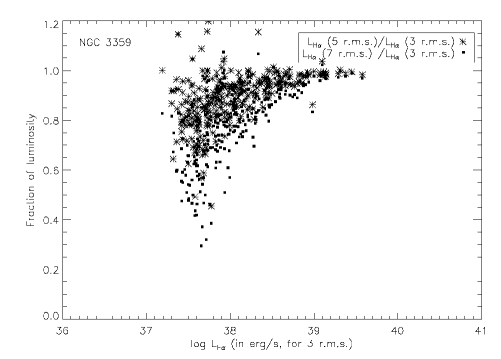
Figure 10: Ratio of the measured luminosity for the H ii regions of NGC 3359 using a cut–off isophote equal to 5 (stars) and 7 (filled squares) times the r.m.s. noise plus the background level of the H$\alpha$ image of the galaxy, to the luminosity measured using 3 times the r.m.s. noise plus the background level.

Although we believe that the data contained in Figs. 9 and 10 demonstrate that the technique we have adopted is reliable, it is still worth seeing the effect of varying the parameters of the different cut–off criteria on the log L_Hα–log $\sigma_{\rm nt}$ relation, using NGC 3359 as a test galaxy. In Table 11 we present the results of this exercise for NGC 3359. We can see that varying the cut–off by changing from 3 times to 5 or 7 times the r.m.s. noise above background gives no significant change in the slope of the lower envelope to the log L_Hα–log $\sigma_{\rm nt}$ diagram, but there is a slight trend to reduced slopes when the alternative criterion using a fraction of the peak brightness as cut–off is used to determine the H$\alpha$ flux, which is as expected from Fig. 10.

Table 11: Slope of the envelope of the log L_Hα-log $\sigma_{\rm nt}$ relation for the H ii regions of NGC 3359 from H ii region catalogues obtained using different criteria to estimate the H ii region cut–off isophote (column 1). The slopes (columns 2 and 4) have been obtained with the procedure described in Sect. 6.2, and each value represents the median value of the slopes obtained by stepping the starting luminosity in the luminosity bins by 0.01dex. Columns 2 and 4 show the median value when taking into account only H ii regions with luminosities greater than log L${}_{\scriptsize{\mbox{H}}\alpha}>$38.4 and 38.8 (in erg s^-1) respectively. The standard deviation of each set of slopes is given in columns 3 and 5. Column 6 shows the completeness limit of the H ii region catalogue obtained for each cut–off isophote criterion. The symbol “–” means that there are not enough points to fit an envelope in that case.

Cut–off	for log LHα$>38.4$		for log LHα$>38.8$		Complet.
isophote	slope	stdev	slope	stdev	limit
I${}_{\rm peak}/$e	1.18	0.08	1.2	0.2	37.4
0.5Ipeak	1.2	0.2	–	–	37.4
3 r.m.s.	1.4	0.3	1.4	0.3	37.1
5 r.m.s.	1.5	0.2	1.4	0.3	37.2
7 r.m.s.	1.5	0.2	1.4	0.3	37.4

We have repeated this exercise for NGC 1530, where the image has a considerably lower signal to noise ratio. In this case the slopes obtained using all four criteria stated above converge to comparable values. This is because the higher noise in the image causes the cut–off levels at 5 and 7 times the r.m.s. noise to approach (and even in some cases slightly exceed) the levels at $1/e$ and $1/2$ of the central peak surface brightness. We note in Tables 11 and 12 that the completeness limits vary according to the cut–off criteria, and that we should be careful not to make comparisons unless the stated lower limiting luminosity of our sample is above the completeness limit for the case chosen. Thus the slopes cited in column 2 of each table are valid only for the cut–off levels at I${}_{\rm peak}/e$, and I${}_{\rm peak}/2$, and at 3 times r.m.s. noise level above the background.

Table 12: Same as Table 11 but for the H ii regions of NGC 1530.

Cut–off	for log LHα$>38.4$		for log LHα$>38.8$		Complet.
isophote	slope	stdev	slope	stdev	limit
I${}_{\rm peak}/$e	2.2	0.2	2.4	0.3	38.2
0.5Ipeak	2.3	0.3	2.6	0.5	38.1
3 r.m.s.	2.0	0.2	2.1	0.6	38.2
5 r.m.s.	2.9	0.4	2.5	0.4	38.4
7 r.m.s.	3.3	0.5	2.4	0.7	38.5

We can conclude as a result of the exercises presented in this Appendix that the use of different criteria for estimating the areas of H ii regions in H$\alpha$ images does produce a significant effect on the derived luminosities of the regions, an effect which is not constant, nor even linear, but varies systematically with the luminosity of the region. From Figs. 9 and 10 we can see that the use of a cut–off at three times the r.m.s. noise is the method of choice for defining the area of an H ii region. It permits more accurate comparisons between authors when data of different quality and depth are used. In high sensitivity exposures the use of a cut–off based on a fixed fraction of peak intensity leads to envelopes with shallower slopes in a log L_Hα–log $\sigma_{\rm nt}$ diagram, and this reflects the fact that this method does not include a significant fraction of the total luminosities of the most luminous regions. Although the two methods converge for images of lower quality this is not sufficient reason to eschew the technique used in the present paper.

- (1) Arsenault, R., & Roy, J. R. 1986, AJ, 92, 567
- (2) Arsenault, R., & Roy, J. R. 1988, A&A, 201, 199
- (3) Arsenault, R., Roy, J.-R., & Boulesteix, J. 1990, A&A, 234, 23
- (4) Böker, T., Calzetti, D. Sparks, W., & et al. 1999, ApJS, 124, 95
- (5) Cepa, J., Beckman, J. E. 1989, A&AS, 79, 41
- (6) Chu, Y-H., & Kennicutt, R.C. 1994, ApJ, 425, 720
- (7) de Vaucouleurs G., de Vaucouleurs A., Corwin H. G., & et al. . 1991, Third Reference Catalogue of Bright Galaxies (RC3), Springer, New York
- (8) Dyson, J. E. 1979, A&A, 73, 132
- (9) Gallagher, J. S., & Hunter, D. 1983, ApJ, 274, 141
- (10) Giammanco, C., Beckman, J. E., Zurita, A., Relaño, M. 2004, A&A, 424, 877
- (11) Hippelein, H.H. 1986, A&A, 160, 374
- (12) Knapen, J. H., Arnth–Jensen, N., Cepa, J., Beckman, J. E. 1993, AJ, 106, 56
- (13) Knapen, J. H. 1997, MNRAS 286, 403
- (14) McCall, M. L., Hill, R. & English, J. 1990, AJ, 100, 193
- (15) McCall, M. L., Straker, R. W., Uomoto, A. K. 1996, AJ, 112, 1096
- (16) Massey, P., Parker, J. W., & Garmany, C. D. 1989, AJ, 98, 1305
- (17) Melnick, J. 1977, AJ, 213, 15
- (18) Melnick, J., Moles, M., Terlevich, R., & García-Pelayo, J.M. 1987, MNRAS 226, 849
- (19) O’Dell, C. R., & Townsley, L. K. 1988, A&A, 198, 283
- (20) Osterbrock, D. E. 1989, Astrophysics of Gaseous Nebulae and Active Galactic Nuclei, (Mill Valley: University Science Books)
- (21) Oke, J. B. 1990, AJ, 99, 1621
- (22) Relaño, M., Peimbert, M., & Beckman, J. E. 2002, ApJ, 564, 704
- (23) Roy, J.-R., Arsenault, R., & Joncas, G. 1986, ApJ, 300, 624
- (24) Rozas, M., Beckman, J. E., & Knapen, J. H. 1996, A&A, 307, 735
- (25) Rozas, M., Sabalisck, N., Beckman, J. E., & Knapen, J. H. 1998, A&A, 338, 15
- (26) Rozas, M., Zurita, A., Heller, C. H., & Beckman, J. E. 1999, A&AS, 135, 145
- (27) Rozas, M., Zurita, A., Beckman, J. E., & Pérez, D. 2000a, A&AS,142, 259
- (28) Rozas, M., Zurita, A., & Beckman, J. E. 2000b, A&A, 354, 823
- (29) Rozas, M., Relaño, M., Zurita, A., & Beckman, J. E. 2002, A&A, 386, 42
- (30) Salpeter, E. E. 1955, ApJ, 121, 161
- (31) Sandage, A., & Tamman, G. A. 1974, ApJ, 190, 525
- (32) Skillman, E., & Balick, B. 1984, ApJ, 280, 580
- (33) Smith, M., & Weedman, D. 1970, AJ, 161, 33
- (34) Spitzer, L. 1978, Physical Processes in the Interestellar Medium, (New York: J. Wiley & Sons)
- (35) Terlevich, R., & Melnick, J. 1981, MNRAS 195, 839
- (36) Tenorio-Tagle, G. 1979, A&A, 71, 59
- (37) Vacca, W.D., Garmany, C. D., & Shull, M. 1996, ApJ, 460, 914
- (38) Vila-Costas, M. B., & Edmunds, M. G. 1992, MNRAS 259, 121
- (39) Yang, H., Chu, Y. -H., Skillman, E. D., & Terlevich, R. 1996, AJ, 112, 146
- (40) Zaritsky, D., Kennicutt, J. R., & Huchra, J. P. 1994, ApJ, 420, 87
- (41) Zurita, A., PhD. Thesis, Univ. La Laguna, 2001
- (42) Zurita, A., Rozas, M., Beckman, J. E 2001, A&A, 363, 9
- (43) Zurita, A., Relaño, M., Beckman, J. E., & Knapen, J. H. 2004, A&A, 413, 73