Characterisation of extrasolar planetary transit candidates

The detection of transits is an efficient technique to uncover faint companions around stars. The full characterisation of the companions (M-type stars, brown dwarfs or exoplanets) requires high-resolution spectroscopy to measure properly masses and radii. With the advent of massive variability surveys over wide fields, the large number of possible candidates makes such a full characterisation impractical for all of them. We explore here a fast technique to pre-select the most promising candidates using either near-IR photometry or low resolution spectroscopy. We develop a new method based on the well-calibrated surface brightness relation along with the correlation between mass and luminosity for main sequence stars, so that not only giant stars can be excluded but also accurate effective temperatures and radii can be measured. The main source of uncertainty arises from the unknown dispersion of extinction at a given distance. We apply this technique to our observations of a sample of 34 stars extracted from the 62 low-depth transits identified by OGLE during their survey of some 10⁵ stars in the Carina fields of the Galactic disc. We infer that at least 78% of the companions of the stars which are well characterised in this sample are not exoplanets. Stars OGLE-TR-105, OGLE-TR-109 and OGLE-TR-111 are the likeliest to host exoplanets and deserve high-resolution follow-up studies. OGLE-TR-111 was very recently confirmed as an exoplanet with M_planet $\cong$ 0.53 $\pm$ 0.11 M_Jup (Pont et al. 2004), confirming the efficiency of our method in pre-selecting reliable planetary transit candidates.

1 Introduction

The search for extra-solar planets (exoplanets) is becoming increasingly important, yielding new insights both in stellar and planetary physics (e.g. Gonzalez 2003). Whilst some studies (Lineweaver & Grether 2003) suggest that 100% of Sun-like stars may have planets, current surveys appear to be heavily biased by the detection techniques used. The radial velocity technique has proved to be extremely successful over the past decade in discovering exoplanets, even though few planetary characteristics can be derived from the measurements. In contrast, planetary transits may yield many more properties, provided the host stars are well characterised. While transit surveys may monitor many orders of magnitude more stars in a comparatively shorter observing time than radial velocity surveys, they are not devoid of problems. Blending, grazing eclipses and contamination by giant stars, among other problems, make some detections somewhat ambiguous (Dreizler et al. 2002, Brown et al. 2001, Drake 2003, Drake & Cook 2004). Clearly transit surveys have the ability to discover many interesting exoplanet candidates, but non-planetary events must be filtered out. The best way to perform such a separation is to obtain radial velocities at different phases along the orbit. Whilst this approach is becoming very successful (Dreizler et al. 2002, Konacki et al. 2003, Bruntt et al. 2003, Street et al. 2003, Bouchy et al. 2004), precision radial velocities for all transit candidates, especially those at faint magnitudes, would be far too time consuming, and so pre-selections must be carried out. For instance, Dreizler et al. (2002) made a selection of the best planetary candidates by using low dispersion spectroscopy to refine stellar parameters, while Drake (2003) used the gravity darkening dependence of the light curves. Another possibility is near-IR photometry which can also be used to discard giant stars, stars with IR excess, and to better determine stellar parameters (e.g. see Ribas et al. 2003, for the case of bright stars with 2MASS photometry) and thus the radii of the companion objects. Ellipsoidal variability is also a good way to filter out the larger companions, although the correlation in the photometric time series limits in practice its applicability (Sirko & Paczyńsky 2003).

The characterisation of the companions and their host stars is thus important for two main reasons. First, it allows a pre-selection of the most promising exoplanet candidates, and filters out giant stars and large companions. Second, the depth of the transits depends upon $R_{c}/R_{*}$, the ratio of the radius of the companion $R_{c}$ to the one from the host star $R_{*}$. Yet the most important and interesting quantity in the case of exoplanets is the radius $R_{c}$, as it allows inferences on the planet’s composition and evolutionary history. Characterising the properties of the host star, and in particular its radius $R_{*}$ is therefore very important for transit candidates.

In this work we explore the possibility to characterise, through IR photometry and low dispersion spectroscopy, the properties of low-luminosity stars whose transits were discovered by the OGLE-III collaboration (Udalski et al. 2002b), in order to constrain astrophysical parameters of both stellar and companion objects, some of which may be exoplanets.

In Sections 2 and 3 we present the observations and data reduction. We describe the estimation of stellar parameters in Section 4 through a novel application of the surface brightness method. The inferred properties of the companions are discussed in Section 5. A brief discussion of the stellar populations observed in these fields is provided in Section 6 with the help of a model of the Galaxy.

2 Observations

In 2002 the second “planetary and low luminosity” companion catalogue was published by the Optical Gravitational Lensing Experiment (OGLE). In this campaign, the OGLE team observed 3 fields in the Carina region of the Galactic disc. These fields were monitored in February–May 2002 searching for low-depth transits in about 100000 stars, and 62 objects were discovered with transit depths shallower than 0.08 mag in the $I$ band. Many of these objects may be extrasolar planets, brown dwarfs or M-type stars (see Udalski et al. 2002b for further details). In order to characterise both stars and companions, we carried out IR imaging and optical spectroscopy in the two Carina fields (Table 1). Table 2 lists the schedule of observations for the subset of planetary transit candidates analysed in this paper.

2.1 Optical $VI$ imaging from OGLE

The optical photometry in the $V$ and $I$ bands come from the catalogue by OGLE (Udalski et al. 2002b), whose observations were carried out with the 1.3m Warsaw telescope at the Las Campanas Observatory, Chile (operated by the Carnegie Institution of Washington). The camera used was a wide field CCD mosaic of eight 2048 $\times$ 4096 pixel SITe ST002A detectors, with a field of view of about 35′$\times$35′  giving a scale of 0$\aas@@fstack{\prime\prime}$26 per pixel. The data were obtained during 76 nights starting from February 17, 2002. The fields were monitored $\sim$ 6 hours per night in the I-band filter with 180 seconds exposure time for each image. The median seeing for the all data was about 1$\aas@@fstack{\prime\prime}$2. The names and coordinates for the observed fields are provided in Table 1.

2.2 $K$-band imaging

We have acquired photometric data in the $K$ band for the CAR 104 and CAR 105 fields. Observations of each field covered an area 35′$\times$45′  with the centres listed in Table 1. Exposure times were 3 seconds per image. The images were taken typically at airmass $\approx$ 1.2 and the limit magnitude was $K\approx$ 17.

These images were taken on January 18, 2003, as a backup program, with the SOFI near-IR array at the 3.5m New Technology Telescope at the ESO La Silla Observatory in Chile. The detector was a Hawaii HgCdTe 1024 $\times$ 1024 array with a scale of 0$\aas@@fstack{\prime\prime}$29 per pixel and a field of view of 5′$\times$5′. The gain was $\sim$ 5.6 e^-/ADU and the readout noise 2.5 ADU.

2.3 Low resolution spectroscopy

The spectroscopy was carried out at the Magellan II 6.5m Clay telescope equipped with the Low Dispersion Spectrograph S2 (LDSS2), during the nights of May 10 and 11, 2003. The data were acquired as a backup program on bright nights, with some thin cirrus and seeing of the order of 1 arcsec. We used the 1″ wide slit, with the high resolution grating which gives 6 Å  resolution and a spectral coverage from 3700 Å  $<\lambda<$ 7500 Å. The spectra were taken at low airmass ($<$1.2), and the exposure times ranged from 90 sec to 600 sec for these relatively bright stars ($14.4\leq V\leq 18.1$). A HeNeAr lamp exposure was acquired immediately after each star’s spectrum. We managed to observe a dozen of sources selected from the list of OGLE candidates (Table 2).

3 Data reduction

3.1 Optical Photometry from OGLE

We used the standard, pipeline-reduced data from OGLE-III (second “planetary and low-luminosity object transit” release, see Udalski et al. 2002a, 2002b). The light curves were produced by a difference image analysis (DIA), and the calibration was done using the OGLE-II and OGLE-III data with errors that should not exceed 0.1–0.15 mag. The very precise DIA photometry of some 100,000 stars yielded 62 objects with shallow dips in their light curves, suggesting flat transits.

3.2 IR photometry

The reduction of the $K$-band data included flat-field and sky substraction, which was carried out with IRAF. The sky frame, which was first subtracted from each image, was made by median-combining 3 to 4 adjacent images. The subsequent flat-fielding was done with a master-flat made from all the frames in the mosaic. The instrumental magnitude was calculated with Sextractor (Bertin & Arnouts 1996) using a median FWHM of about 2.7 pixels for all the stars. The aperture radius was 1 FWHM and the background was taken at 2 FWHM. The zero point calibration was done using the 2MASS (2 Micron All Sky Survey) database. We required a match between the position of our stars and the 2MASS stars within 1″  in RA and DEC. Our magnitude range was between $11<K<17$ and the error in the zero point calibration was about 0.05 (median for this filter calculated by 2MASS). Note that the error shown in Table 3 does not include the zero point error. The $K$-band zero point determined was $Z_{p}$= 23.43. For the $V$ magnitude, we matched the published list by Udalski et al. (2002b) and a list delivered by the OGLE project in which we have the photometric $V$ and $I$ magnitudes and coordinates for all the stars in the two fields. Because the fields are somewhat crowded, some candidates were surrounded by other stars and the match failed. Table 3 summarises the photometry for the target stars. Column 1 gives the stellar ID from Udalski et al. (2002b), columns 2 and 3 the optical $VI$-band photometry from OGLE, and column 4 our $K$-band photometry along with its error. Other columns are discussed later on. The target stars have $14.3\leq V\leq 18.65$, and $12.17\leq K\leq 16.4$. The resulting optical-infrared colour-colour diagram is given on Figure 1.

3.3 Spectroscopy

From the images of the spectra we have subtracted a combined bias, trimmed and divided by a combined normalised flat-field obtained from high S/N quartz lamps. The spectra were extracted using IRAF tasks within the TWODSPEC package, with their background properly removed. The wavelength calibration was done with the HeNeAr lamps, using 14 to 20 lines. The cosmic rays were excised, and the spectra were flux calibrated using the spectrophotometric standards. However the flux calibration is unreliable because of the presence of thin cirrus during the nights. The final spectra are plotted in Figure 2. Although a qualitative spectral classification can be made by comparing these spectra with a series of templates (e.g. Dreizler et al. 2002), we prefer to measure the effective temperatures using the three most intense lines from the Balmer series. The results are summarised in Table 4, and Figure 3 shows that the independent measures from different Balmer lines is in excellent agreement. The weighted mean of the three effective temperatures is given in Column 8 of Table 4, while the measured radial velocities are given in Column 9.

4 Determination of stellar parameters

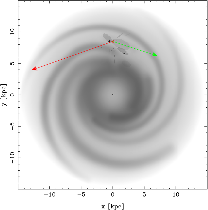
Figure 4: Location of the Carina fields (leftwards arrow) and the field proposed for the Kepler mission (rightwards arrow) within the spiral arms of the Galaxy, as traced by the distribution of free electrons (Cordes & Lazio 2003). The Carina line of sight clearly crosses the Carina-Sagittarius arm in at least two places, at about 2 and 7 kpc from the Sun. In comparison, the Kepler field crosses the Perseus arm at a much larger distance of 6 kpc.

The determination of the properties of the stars which have transits, based solely on optical and $K$-band photometry and on low-resolution spectroscopy, is complicated by the lack of information on the extinction along their lines of sight. Even though the Carina fields (Table 1) correspond to regions of the Galactic disc where the reddening and extinction are relatively low, locally, they cross the Carina-Sagittarius spiral arm at least twice, as shown on Fig. 4 where the arms were traced with the distribution of free electrons as determined by dispersion measures on pulsars (Taylor and Cordes 1993, Cordes and Lazzio 2003). Extinction is extremely patchy in these regions of the Carina arm (Wramdemark 1980), which are populated by many star-forming complexes and cavities (Georgelin et al. 2000), leading to a wide range not only of extinction values but also of the reddening parameter $R_{\mathrm{V}}$, which in these areas ranges from 3.0 to 5.0, with an average of about 4.0 (Patriarchi, Morbidelli & Perinotto 2003), much larger than the anomalous ones seen in the bulge (Udalski 2003).

Since the target stars presumably lie, given their magnitudes and spectral types, on the first intersection with the Carina spiral arm, we estimate the reddening along the line of sight with the 3-dimensional model by Drimmel et al. (2003) as a guide. Figure 5 shows the colour excess $E(B-V)$  as a function of distance (assuming $R_{\mathrm{V}}$ = 3.1) predicted by this model for the two fields considered in this study, along with the one assumed by the Besançon Galaxy model which we will use later on to analyse the field population (Section 6). This improves upon the estimation made by Mendez & van Altena (1998), and appears to be the only practical guide at low galactic latitudes. The Drimmel et al. (2003) 3-dimensional model predicts two important features long these directions (see Fig.  5). First, the intersection with the spiral arm is reflected by the rapid increase in the absorption at about 2 kpc, and then at about 6.5 kpc, fully consistent with the map shown on Fig. 4. The Besançon Galaxy model is, in comparison, less realistic as this feature is not present. Second, the predicted colour excess at 8 kpc appears extremely large, between 1.4 and 1.7 magnitudes in $E(B-V)$, while the Besançon Galaxy model reaches an asymptote well below 1 magnitude. The reason of this discrepancy is unclear, but may perhaps be related to the fact that the 3-D model is calibrated on the data of DIRBE/COBE and ISSA/IRAS which may overestimate the reddening by factors up to 1.5 in regions where $A_{\mathrm{V}}$$>0.5$ mag (Arce & Goodman 1999). We also note that simple, homogeneous exponential discs will produce an extinction of the form

$$A_{\mathrm{V}}\;=\;\left(\frac{\kappa_{o}}{10\,\sin|b|}\right)\,\left(1-\exp\left[\,-10\,d\,\sin|b|\right]\right)$$ (1)

where $d$ is measured in kpc, so that asymptotically when $b\to 0$ the extinction tends to $\kappa_{o}$ magnitudes per kpc. The Besançon Galaxy model appears to give a distance dependent extinction similar to an exponential disc with $\kappa_{o}=1.05$ (Fig. 5). To simulate and account for the effect of a possible increase of $R_{\mathrm{V}}$  as large as 4, we will also use $\kappa_{o}=0.70$. Note that while the extinction predicted by this series of models at large distances is very different, below 2 kpc the range becomes rather narrow, and the results will largely be independent of the assumed extinction. At large distances, the unknown dispersion of $A_{\mathrm{V}}$  at a given distance will be a limiting factor.

The simultaneous measure of $R_{\mathrm{V}}$  and $E(B-V)$  independently would require a much better absolute flux calibration of the low resolution spectra and $U$-band photometry or UV spectra, and is clearly beyond the scope of this work. We will assume instead $R_{\mathrm{V}}$$=3.1$ and consider a variety of extinctions to account both for a possible variation of $R_{\mathrm{V}}$  and the dispersion of extinction at a given distance. To determine the extinction of each star, the colour-colour diagrams (Fig. 1) cannot be used, because the reddening vector happens to have the same direction as the locus of the main sequence stars, and even some giants may also lie close to the sequence.

One possibility would be to compute reddening-independent indices based on the standard dependence of extinction with wavelength. For instance,

$$Q_{\mathrm{VIK}}\;=\;(V-I)\,-\,\left[\frac{E(V-I)}{E(I-K)}\right]\,(I-K)$$ (2)

where

$$E(V-I)\; = \;A_{\mathrm{V}}\,\left(1.0-\frac{A_{\mathrm{I}}}{A_{\mathrm{V}}}\right)$$ (3)

$$E(I-K)\; = \;A_{\mathrm{V}}\,\left(\frac{A_{\mathrm{I}}}{A_{\mathrm{V}}}-\frac{A_{\mathrm{K}}}{A_{\mathrm{V}}}\right)$$ (4)

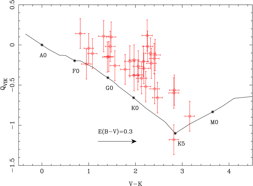
Figure 6: Reddening-free index $Q_{\mathrm{VIK}}$ as a function of the observed $V-K$ colour. The solid line gives the theoretical locus of unreddened main sequence stars. Note the systematic horizontal offset produced by reddening, whose average colour excess E(B-V) of about 0.3 magnitudes is indicated by the horizontal arrow.

and we adopt $A_{\mathrm{I}}/A_{\mathrm{V}}=0.479$ and $A_{\mathrm{K}}/A_{\mathrm{V}}=0.113$ (Cardelli et al. 1989). The resulting diagram is shown on Fig. 6 where the horizontal shift produced by extinction is clearly visible and amounts, in average, to about $E(B-V)$$=0.3$. If all the stars were on the main-sequence, the reddening would be measured through the horizontal shift required to move the observed position to the main sequence locus. Unfortunately we have no guarantee that all these stars are on the main sequence of solar metallicity, as some may be more metal rich and some giants could well be present, especially in the lower half of the diagram. Clearly another technique has to be used to measure unambiguosly the reddening.

In this paper we introduce a new method based on the well-known surface brightness (SB) relation which has been recently recalibrated using exclusively direct interferometric measures of angular diameters (Kervella et al. 2004). The surface brightness $S_{\lambda}$ in a given passband is just

$$S_{\lambda}\;=\;a\,-\,0.1m_{{\lambda}_{o}}\,-\,0.5\log\,\theta_{\mathrm{LD}}$$ (5)

where $m_{{\lambda}_{o}}$ is the intrinsic, dereddened apparent magnitude in that passband and $\theta_{\mathrm{LD}}$ its limb-darkened angular diameter. Since the surface brightness is tighly correlated to colour, the equation can be inverted to yield the diameter as a function of colour. Our method has thus three distinct steps. First, a distance is assumed, and hence a reddening (based on the model adopted for extinction). Magnitudes and colours are dereddened. The resulting optical and IR magnitudes are used to infer the limb darkened angular diameter of the star, via the relations

$$\log\,\left(\frac{\theta_{\mathrm{LD}}}{\mathrm{mas}}\right) = 0.5170\,+\,0.0755(V-K)_{o}\,-\,0.2K_{o}$$ (6)

$$\log\,\left(\frac{\theta_{\mathrm{LD}}}{\mathrm{mas}}\right) = 0.5149\,+\,0.1805(I-K)_{o}\,-\,0.2K_{o}$$ (7)

where the rms dispersions are less than 1% and 3.7% respectively (Kervella et al. 2004). Our final estimate is the weigthed mean of these two estimates.

The second step estimates the effective temperature through the relation

$$\log T_{\mathrm{eff}}\;=\;4.1788$$

$$-\,\left[1.1806\log\theta_{\mathrm{LD}}\,+\,0.2361K_{o}\,-\,0.5695\right]^{1/2}$$

with a dispersion smaller than 0.6%, which corresponds to a systematic error of 40 K for a G2 V star (Kervella et al. 2004). The combination of the first two steps yields an estimate of the effective temperature which depends on the assumed distance. It also yields directly the intrinsic stellar radius as

$$\left(\frac{R_{*}}{R_{\odot}}\right)\;=\;4.434\,10^{10}\;\left(\frac{d}{\mathrm{kpc}}\right)\;\tan\left(\frac{\theta_{\mathrm{LD}}}{2}\right)$$ (9)

The third and last step makes use of the properties of main-sequence stars : the strong correlation between luminosity and mass ($L\sim M^{\beta}$), and between mass and radius ($M\sim R^{\alpha}$), and hence between effective temperature and radius of the form

$$\left(\frac{T_{\mathrm{eff}}}{T_{\mathrm{eff}\odot}}\right)\;=\;\left(\frac{R_{*}}{R_{\odot}}\right)^{\left(\alpha\beta-2\right)/4}\;\approx\;\left(\frac{R_{*}}{R_{\odot}}\right)^{0.64}$$ (10)

using the standard values of $\alpha=1/0.8$, $\beta\approx 3.6$ and $T_{\mathrm{eff}\odot}=5770$ K. The resulting dependence of this new estimate of the effective temperature with the distance will clearly be different from the one resulting from the surface brightness relation. If a distance exists such that both estimates agree, we have a full solution with all the parameters of a main sequence star that agrees with the optical and IR photometric data. If there is no solution, then either the star is a giant, for which the surface brightness relations that we have used do not apply, or the assumed reddening at that distance is incorrect.

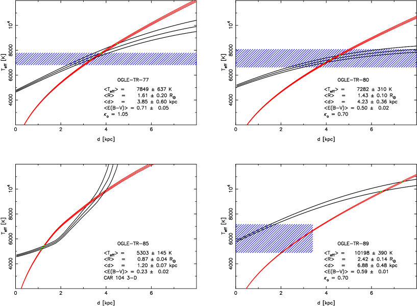
Figure 7: Effective temperature versus distance for selected candidates (OGLE-TR-77, OGLE-TR-80, OGLE-TR-85, OGLE-TR-89). The red lines show the radius-temperature constrain for main sequence stars, weakly dependent on photometrical errors, while the black lines give the range of temperatures inferred from the surface brightness relation when the errors in the $V-K$ colours and $V$ magnitudes are considered. If present, the blue hatched region give the range of effective temperature allowed by the main Balmer lines. A colour figure is available in the electronic version of the paper.

The procedure is illustrated in Fig. 7 for 4 candidates from the OGLE list. In the case of OGLE-TR-77, the three black lines give the effective temperature as a function of distance (assuming $\kappa_{o}=1.05$) for the mean and the two extreme values of the optical and K-band magnitudes. The relatively large separation between these three estimates is due to the large uncertainties (0.10–0.15 mag) in the OGLE optical magnitudes. The red lines give the constraint from the main sequence (Eq. 10) which appears to be far less sensitive to the photometrical errors. The intersections of the lines yield a unique and accurate solution for the effective temperature, the stellar radius, the distance and the reddening.

A fully independent estimate comes from the measures of the effective temperatures based on the low-resolution spectra (Table 4). When available, these measures are indicated on Figs. 7 to 10 as a hatched band, independent of distance. As shown on Fig. 7 the agreement for OGLE-TR-77 and OGLE-TR-80 is impressive.

The method is not devoid of problems, however. As Fig. 7 illustrates, in the case of OGLE-TR-85 two solutions are possible, and there is no way to select the correct one on the basis of that information only. However, the value of the reddening-free index $Q_{\mathrm{VIK}}$ indicates that OGLE-TR-85 must have a spectral class between G2 and K0 (Fig. 6) and hence the short distance solution is preferred. The steep increase in the SB-derived temperatures in this case was produced by the steep increase in extinction predicted by the 3-D extinction model by Drimmel et al. (2003). Other models would not give the second solution, as at that distance the expected scatter in reddening is very small, and so, again, the short distance solution is preferred.

A second problem arises when the temperatures derived from the SB relation do not agree with the spectroscopic ones. This is the case for OGLE-TR-89 (Fig. 7) where the SB-inferred temperature gives a temperature of some 10,000 K while the spectrum indicates 6,000 K. Again the reddening-free index $Q_{\mathrm{VIK}}$ (see Fig. 6) indicates that the position of OGLE-TR-89 is consistent with the locus of A-type stars, pointing either to a problem in the spectrum or else that it is a giant star, in which case the SB-inferred temperature is of course incorrect. The latter explanation is likely, as the SB method points to a large distance (6.9 kpc) which is very unlikely for this bright star.

While at distances below 2 kpc the inferred measures are independent of the reddening assumed at these distances (Fig. 5), at larger distances there is a rather strong dependence on the assumed extinction. For instance, in the case of OGLE-TR-89 or OGLE-TR-118, an extinction larger than the one predicted by the $\kappa_{0}=0.7$ exponential model would yield either a very large distance, which is unlikely given their magnitudes, or no solution at all, pointing to supergiant stars.

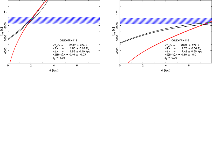
Figure 10: Same as Fig. 7 for OGLE-TR-112 and OGLE-TR-118. A colour figure is available in the electronic version of the paper.

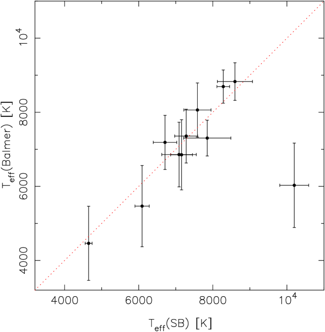
Figure 11: Comparison of effective temperatures derived from the Balmer lines and from the surface brightness method. The only outlier is OGLE-TR-89, which is very likely a giant star.

In general, the agreement between the SB-inferred temperatures and the spectroscopic ones is very good, as illustrated on Figure 11. The only outlier is, in fact, OGLE-TR-89 which is likely to be a giant star, as discussed above. Likewise, the large distance inferred for OGLE-TR-118 (see Fig. 10) makes it likely to be a giant star.

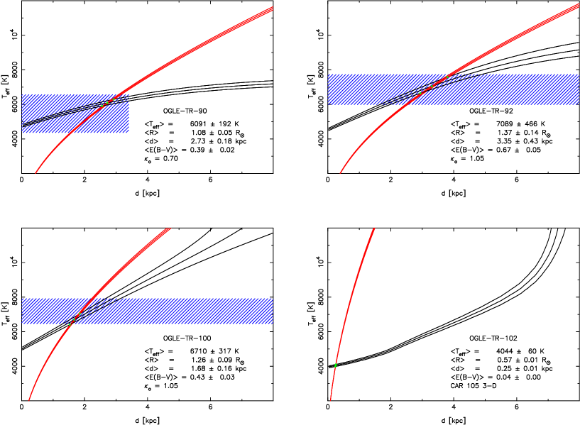
Figure 8: Same as Fig. 7 for OGLE-TR-90, OGLE-TR-92, OGLE-TR-100 and OGLE-TR-102. A colour figure is available in the electronic version of the paper.

Some other stars deserve comments. OGLE-TR-102 (Fig. 8) appears to have a solution with a very short distance (0.25 kpc), as appropriate for such a low temperature star inferred from the SB method. This temperature is fully consistent with its small $Q_{\mathrm{VIK}}$ index which makes it a late main-sequence K star (Fig. 6). Yet its position on the colour-magnitude (Fig. 14) shows that it could also be a giant star, at of course a much larger distance. The Galaxy model that we will use in §6 shows that such a small distance is not expected in a sample of stars of this size, providing yet another hint that this star is a giant.

In summary, OGLE-TR-83, OGLE-TR-98, OGLE-TR-116 and OGLE-TR-119 do not yield any solution and are therefore very likely to be giant stars. As their main-sequence solutions yield large distances, OGLE-TR-89 and OGLE-TR-118 are also likely to be giants. OGLE-TR-102 is also likely to be a giant, even though a reasonable value for its parameters, consistent with all the data, is found assuming that it is a main-sequence star. Table 5 summarises the stellar properties inferred from our method.

Further refinements would require intermediate resolution spectroscopy. For instance, the measure of the KP (metallicity-dependent) and HP2 (pseudo-EW of the Balmer H_δ line) indices would allow the colour excess to be measured within 0.03 mag (Bonifacio, Caffau & Molaro 2000) independently of any assumption on distance (although $R_{\mathrm{V}}$  cannot be measured in this way). Even though it is less costly in telescope time than high resolution spectroscopy, it remains unpractical for a large systematic follow-up survey.

5 Constraints on the companions

The main objective of our observations is to better characterise the properties of the host stars in order to infer the radii of their companions. They are given straightforwardly through the standard relation (e.g. Seager & Mallén-Orlenas 2003)

$$\left(\frac{R_{c}}{R_{*}}\right)\;=\;\left(10^{\Delta I/2.5}-1\right)^{1/2}$$ (11)

where $\Delta I$ is the depth of the transit in magnitudes in the $I$ band, provided by OGLE and given in Table 5.

Clearly the vast majority of companions are low-mass objects but are not small enough to be exoplanets. If we adopt as an example the first extrasolar planet discovered with the transit technique, HD 209458b (Charbonneau et al. 2000), which is a close giant planet with a radius of 1.35 $\pm$ 0.16 $R_{\mathrm{Jup}}\sim$ 0.14 $R_{\odot}$, only three companions could be exoplanets : OGLE-TR-105, OGLE-TR-109 and OGLE-TR-111.

OGLE-TR-102 is somewhat dubious because the host star is probably a giant star, as discussed above, in which case the stellar radius has been seriously underestimated. In this case the radius of the component has also been underestimated and the odds are that the transiting object is not an exoplanet.

OGLE-TR-105 and OGLE-TR-111 are the best candidates, as the stellar radiii are measured to within 3% and they are clearly main sequence stars with mid-K spectral types. OGLE-TR-105 only had 3 transits measured (Udalski et al. 2002b) and therefore is a bit more dubious that OGLE-TR-111 with 9 measured transits.

OGLE-TR-109 would have the shortest period (below 1 day) and is a borderline object at $R_{c}$=0.13 $R_{\odot}$, along with OGLE-TR-90 and OGLE-TR-100. They all share the property that their host stars are rather hot, with effective temperatures around 7,000 K. Some of the MACHO transit candidates, selected from a subset of 180,000 stars in the MACHO database of the Bulge, also appear around this type of stars (Drake & Cook, 2004)

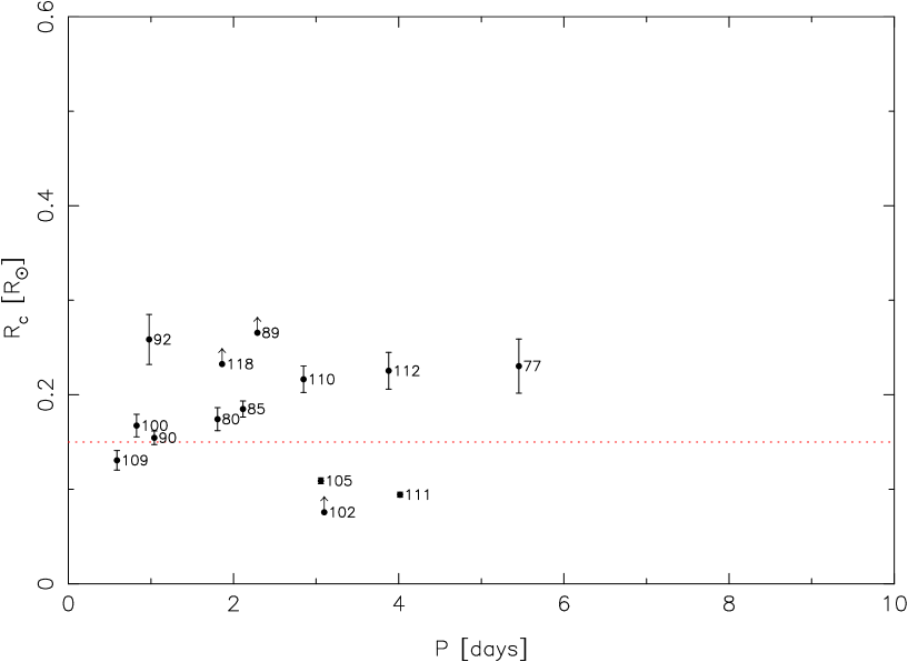
Figure 12: Inferred radii for the companions $R_{c}$ as a function of their orbital period. The dotted horizontal line at 0.15 $R_{\odot}$ marks the adopted transition below which companions are likely to be exoplanets. The arrows indicate the lower limits associated with likely host giant stars. Only three transit candidates appear likely to have exoplanets : OGLE-TR-105, OGLE-TR-109 and OGLE-TR-111.

Figure 12 summarises the results by showing the inferred radii of the companions as a function of their orbital period. The candidates selected here all fall within the category of “hot” Jupiters as their periods are close to 3 days and appear to be quite compact. It is beyond the scope of this work to discuss further the physical properties of this subset of possible candidates.

It is interesting to compare the results of our analysis with the best candidates selected by the OGLE team. They assumed that all the host stars had one solar mass exactly and inferred the corresponding radii of the companions using Eq. 11. Of their 10 best candidates with $R_{c}/R_{\odot}<0.14$ that we observed, only two are confirmed : OGLE-TR-109 and OGLE-TR-111, and one is unclear. Overall, we exclude at least 70% of their best candidates (with $R_{c}/R_{\odot}<0.14$) and possibly 80%. The are two reasons for this: in 30% of the cases the star appears to be a giant, while in the rest our revised radii become too large. In addition, one candidate which had $R_{c}/R_{\odot}=0.16$ appears to have a smaller radius of 0.11 $R_{\odot}$ (OGLE-TR-105) and hence enters in the list of possible exoplanets. This proves the effectiveness of our approach in pre-selecting the best candidates for high-resolution spectroscopy.

6 The stellar populations in the fields

The stellar populations present in the Carina fields not only are interesting in their own right but could also shed some light on the properties of the transit candidates. For instance, in our solar neighborhood many of the confirmed planets orbit around main sequence stars of perhaps slightly larger metallicity than solar (Gonzalez 2003). We have seen (§4) that the distances of the transit stars inferred from the SB method range from about 1 to 4 kpc. Figures 13 and  14 show the candidates and the field population in optical colour-magnitude and optical-IR colour-magnitude diagrams respectively. The Padova isochrones (Girardi et al. 2002) for solar age and metallicity, without reddening, are also indicated at 1 kpc (solid line), 2 kpc (dotted line) and 4 kpc (short dashed line), and confirm that the candidate stars are indeed within this range.

Assuming a solar distance to the Galactic center of $R_{0}=8$ kpc, the location of these fields has a typical distance of 7.5 kpc from the Galactic centre. The stellar population in these fields should not be too different from that of the solar circle. If we consider the metallicity gradient in the Galactic disk of -0.09 $\pm$ 0.02 dex/kpc (Friel & Janes 1993), the mean metallicity in the field should be $\sim$ 0.04 dex larger in the mean than that of the Solar neighborhood. Such a small difference would hardly matter.

Further insights can be gained through the comparison with a synthetic model of the Galaxy. The Besançon model has been updated recently (Robin et al., 2003) and is very convenient for our purposes as we can derive the distribution of stars, their photometric properties and distances in a given direction. In addition, the model provides information on the metallicities and kinematics of these samples. The predicted differences between the two fields, Carina 104 and 105 are small given the sampling fluctuations and the patchy extinction.

From the model, we selected main sequence stars having the same range of $K$-band magnitudes as our candidates. Further, we also selected those with a luminosity class equals to V, that is, on the main sequence. We also applied a cut in metallicity, such that $-0.25<\mathrm{[Fe/H]}<0.5$ but this proves to be not very discriminant, because most stars are within this range, given the metallicity gradient observed in the disc, as discussed above. The question that arises is whether the distributions of inferred distances and colour excesses for the candidates could be sampled from the synthetic model. This is important as we did not use the Besançon model for the dependence of reddening with distance, and hence this comparison provides a good test of the procedure, given the model.

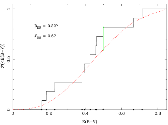
Figure 15: (Top) Distribution function of the $E(B-V)$  colour excess predicted by the Besançon model for main-sequence and giant stars in the range 11.5 $\leq K\leq$ 16.0 and near solar metallicity. Note the gaussian-shaped distribution for main-sequence stars, and the highly skewed distribution for giants, as expected for brighter and hence more distant stars. The cutoff at 0.92 corresponds to the maximal colour excess predicted by the Besançon model. (Bottom) Cumulative distribution functions of colour excess $E(B-V)$  for the OGLE transit stars which are inferred to be main-sequence stars (points and dark line) and for the main sequence stars of the Besançon model selected with the criteria of the top panel (dotted red line). A two-sample Kolmogorov-Smirnov test gives a 57% probability.

The resulting distribution function of the $E(B-V)$  colour excess is given in Figure 15 (Top) where for the sake of completeness we have also indicated the distribution for the giant stars. The gaussian-shaped distribution for the selected main-sequence stars appears very similar to the distribution of the inferred $E(B-V)$  for the candidates (see Table 3), while giant stars present a very skewed distribution, a reflection of the brigher absolute magnitudes and hence larger distances which lead to larger colour excesses, on average. Beyond this qualitative comparison, we can give a quantitative answer to the question of whether the Besançon model could be the parent population out of which the sample of candidates could have been extracted. Figure 15 (Bottom) gives the cumulative distribution functions, and a simple two-sample Kolmogorov-Smirnov test gives a probability of 57% for the two samples to be drawn from the same population. Note that we removed the likely giants from our OGLE sub-sample. Although this probability is not too high, we can conclude that the Besançon model provides a reasonable agreement, especially since we did not use the underlying reddening model.

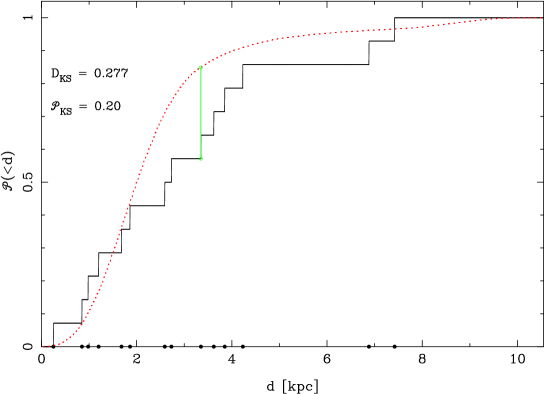
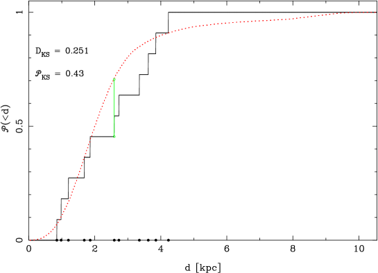
Figure 16: Cumulative distribution functions of distances for the OGLE transit stars with inferred distances (points and dark line) and for the Besançon model with main sequence stars in the range 11.5 $\leq K\leq$ 16.0 (dotted red line). The top panel includes OGLE-TR-89, OGLE-TR-102 and OGLE-TR-118 and has ${\cal{P}}_{\mathrm{KS}}=0.20$ while the bottom panel excludes these three giant stars, yielding a signficantly much higher probability of ${\cal{P}}_{\mathrm{KS}}=0.43$.

A further sensitive test comes from the distribution of distances. Figure 16 shows the cumulative distribution functions of both candidates and synthetic stars (top panel). A Kolmogorov-Smirnov test yields a probability that the sample of candidates is extracted from the parent synthetic population of 20% when we consider all the candidates. If we remove OGLE-TR-102, OGLE-TR-89 and OGLE-TR-118 as likely giant stars, we get a much larger probability of 43%, fully confirming our suspicion that these three stars cannot be drawn from the main-sequence population.

The detailed distribution of stars in the colour-magnitude diagrams depends heavily on the star formation history, the metallicity distribution function and the initial stellar mass function, in addition to the extinction properties mentioned in §4 and the actual density distributions of the thin and thick discs, which are dominant in these fields. While there are methods to infer the past history of star formation from volume-limited samples close to the solar neighbourhood (e.g. Hernandez et al. 2000), such an analysis clearly goes beyond the scope of this paper. We will just note here that a nearby field ($\ell$ = 292.45, $b$=1.63) has yielded interesting constraints on galactic structure (see the field F3 analysed by Vallenari et al. 2000) although the results depend strongly on the assumed age and metallicity range of the populations.

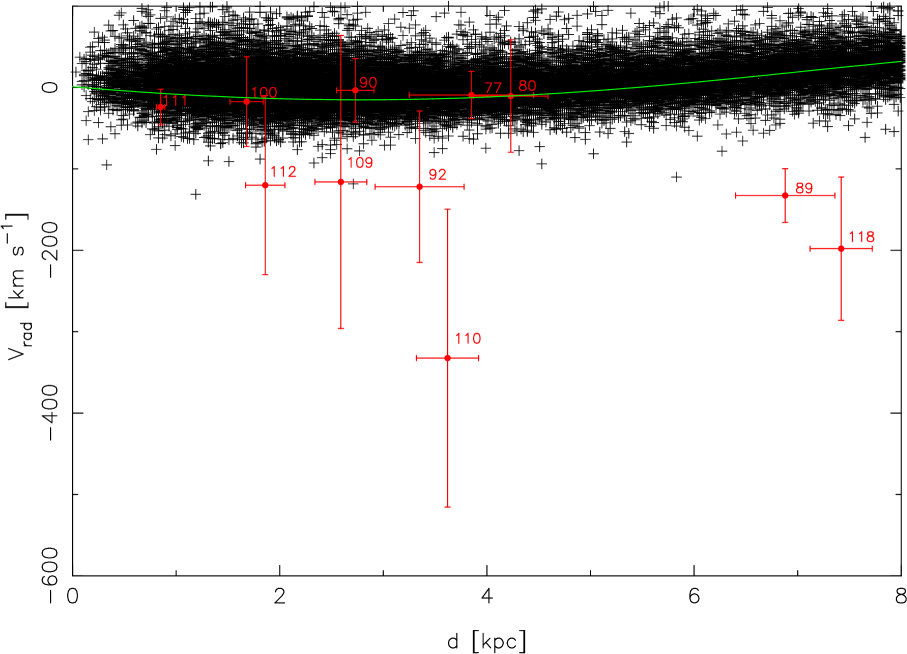
Figure 17: Radial velocity as a function of distance : transit candidates (filled circles with error bars), simulated field stars from the Besançon model (crosses) and mean Hi velocity field (Nakashini & Sofue 2003). While the majority of OGLE candidates are consistent with these models, clearly OGLE-TR-89, OGLE-TR-110 and OGLE-TR-118 cannot be explained within this framework.

Finally, the kinematics of the model can also be tested since we have a few radial velocities measured from the low-resolution spectra (Table 4). Figure 17 gives the radial velocities as a function of the distance along the line of sight for both the candidates and the synthetic stars. The radial velocity along these lines of sight can be also calculated using the accurate model by Nakashini & Sofue (2003) which fits the observed distribution of Hi gas. As expected, most radial velocities are close to zero, and overall there is an excellent agreement, except perhaps for OGLE-TR-89, OGLE-TR-110 and OGLE-TR-118.

We conclude that, even though these data are not sufficient to strongly constraint the structure of the Galaxy along these directions, they are consistent with current models.

7 Conclusions

In order to make an efficient pre-selection of possible exoplanets, we obtained $K$-band photometry for a sample of transit candidates detected by the OGLE collaboration in the CAR 104 and CAR 105 fields of the Galactic disc, along with low-dispersion spectroscopy of 11 promising candidates. By combining these new data with the optical $VI$ photometry from OGLE, we presented a novel application of the surface brightness relations to measure the colour excess of each transit star, its distance, and, more importantly, the effective temperature and radius, and hence to fully caracterise their properties. The method rejects automatically giant stars, and provide accurate solutions for main-sequence stars. A comparison with the temperatures derived from the low-resolution spectra shows an excellent agreement and validates the method. The new measures of stellar radii allow us to further refine the radii of the companions.

We find that :

1. The combination of optical with near-IR photometry allows a very good estimate the stellar parameters for most stars and therefore to select the best planetary transit candidates in a very effective way, bypassing the need of high-resolution spectroscopy at this stage of the selection process.

2. We discard OGLE-TR-83, OGLE-TR-89, OGLE-TR-98, OGLE-TR-102, OGLE-TR-116, OGLE-TR-118 and OGLE-TR-119 for being very probably giant stars.

3. Over 70% of the sub-sample contains low-mass companions whose radii are far too large to be exoplanets.

4. We select OGLE-TR-105, OGLE-TR-109 and OGLE-TR-111 (full squares in Fig. 1, 13 and 14) as the most likely transit candidates to host exoplanets, as the inferred radii of their companions are below $R_{c}/R_{\odot}<0.14$. As their periods are shorter than 3.5 days, these are new possible “hot Jupiter”-like planets.

5. Recently, Pont et al. (2004) confirmed OGLE-TR-111 as an exoplanet with a mass of 0.53 $\pm$ 0.11 M_Jup and a radius of 1.0${}^{1.13}_{0.94}$ R_Jup. Our calculated radius for OGLE-TR-111 is about 0.91 $\pm$ 0.03, showing the reliability of our method to reject “false positives” and efficiently select promising extrasolar planetary transit candidates.

A comparison with the Besançon model of the Galaxy shows a satisfactory agreement and that these stars are normal and representative of the thin disc population.

In the future it would be useful to obtain high-resolution spectra with UVES/VLT for the three candidates to measure radial velocities and to determine accurately their masses.

Table 1: Coordinates of the observed fields.

Field	$\alpha$  (J2000)	$\delta$  (J2000)	l	b
CAR 104	$10{{}^{h}}57^{m}30^{s}$	$-$61°40′00″	289$\aas@@fstack{\circ}$84	$-$1$\aas@@fstack{\circ}$72
CAR 105	$10{{}^{h}}52^{m}20^{s}$	$-$61°40′00″	289$\aas@@fstack{\circ}$29	$-$1$\aas@@fstack{\circ}$99

Table 2: Journal of observations.

Name	$\alpha$  (J2000)	$\delta$  (J2000)	IR Images	Spectra
OGLE-TR-76	10:58:41.90	$-$61:53:12.3	NTT+SOFI 18Jan03	…
OGLE-TR-77	10:58:02.03	$-$61:49:50.9	NTT+SOFI 18Jan03	CLAY+LDSS-2 11May03
OGLE-TR-78	10:59:41.62	$-$61:55:15.0	NTT+ SOFI 18Jan03	…
OGLE-TR-79	10:59:35.54	$-$61:56:59.2	NTT+ SOFI 18Jan03	…
OGLE-TR-80	10:57:54.36	$-$61:42:02.5	NTT+SOFI 18Jan03	CLAY+LDSS-2 11May03
OGLE-TR-83	10:57:42.48	$-$61:36:23.3	NTT+SOFI 18Jan03	…
OGLE-TR-84	10:59:00.00	$-$61:34:43.0	NTT+SOFI 18Jan03	…
OGLE-TR-85	10:59:00.18	$-$61:37:41.1	NTT+SOFI 18Jan03	…
OGLE-TR-87	10:59:39.33	$-$61:24:07.3	NTT+SOFI 18Jan03	…
OGLE-TR-89	10:56:11.27	$-$61:29:55.4	NTT+SOFI 18Jan03	CLAY+LDSS-2 10May03
OGLE-TR-90	10:56:36.63	$-$61:28:46.5	NTT+SOFI 18Jan03	CLAY+LDSS-2 10May03
OGLE-TR-92	10:57:23.43	$-$61:26:45.4	NTT+SOFI 18Jan03	CLAY+LDSS-2 11May03
OGLE-TR-95	10:55:19.38	$-$61:32:12.0	NTT+SOFI 18Jan03	…
OGLE-TR-98	10:56:51.77	$-$61:56:15.0	NTT+SOFI 18Jan03	…
OGLE-TR-99	10:55:12.80	$-$61:54:54.8	NTT+SOFI 18Jan03	…
OGLE-TR-100	10:52:56.91	$-$61:50:54.9	NTT+SOFI 18Jan03	CLAY+LDSS-2 10May03
OGLE-TR-101	10:52:58.59	$-$61:51:43.1	NTT+SOFI 18Jan03	CLAY+LDSS-2 11May03
OGLE-TR-102	10:53:29.65	$-$61:47:37.2	NTT+SOFI 18Jan03	…
OGLE-TR-104	10:53:27.04	$-$61:43:20.3	NTT+SOFI 18Jan03	…
OGLE-TR-105	10:52:24.07	$-$61:31:09.4	NTT+SOFI 18Jan03	…
OGLE-TR-106	10:53:51.23	$-$61:34:13.2	NTT+SOFI 18Jan03	…
OGLE-TR-107	10:54:23.58	$-$61:37:21.1	NTT+SOFI 18Jan03	…
OGLE-TR-108	10:53:12.65	$-$61:30:18.7	NTT+SOFI 18Jan03	…
OGLE-TR-109	10:53:40.73	$-$61:25:14.8	NTT+SOFI 18Jan03	CLAY+LDSS-2 11May03
OGLE-TR-110	10:52:28.37	$-$61:29:31.8	NTT+SOFI 18Jan03	CLAY+LDSS-2 11May03
OGLE-TR-111	10:53:17.91	$-$61:24:20.3	NTT+SOFI 18Jan03	CLAY+LDSS-2 10May03
OGLE-TR-112	10:52:46.46	$-$61:23:17.7	NTT+SOFI 18Jan03	CLAY+LDSS-2 11May03
OGLE-TR-116	10:50:24.79	$-$61:26:12.2	NTT+SOFI 18Jan03	…
OGLE-TR-117	10:51:40.48	$-$61:34:15.7	NTT+SOFI 18Jan03	…
OGLE-TR-118	10:51:32.10	$-$61:48:08.3	NTT+SOFI 18Jan03	CLAY+LDSS-2 11May03
OGLE-TR-119	10:51:58.75	$-$61:41:20.5	NTT+SOFI 18Jan03	…
OGLE-TR-120	10:51:09.34	$-$61:43:11.3	NTT+SOFI 18Jan03	…

Table 3: Observed and derived photometric properties

Name	Va	Ia	Kb	E(B–V)	$V_{o}$	$(V-I)_{o}$	$(V-K)_{o}$	$M_{V}$
OGLE-TR-76	14.30	13.76	13.48 $\pm$ 0.01
OGLE-TR-77	17.46	16.12	15.06 $\pm$ 0.03	0.71 $\pm$ 0.05	15.25 $\pm$ 0.13	0.19 $\pm$ 0.15	0.44 $\pm$ 0.12	2.32
OGLE-TR-78	16.23	15.32	14.75 $\pm$ 0.02	0.52:	14.62:	0.07:	0.05:	1.34:
OGLE-TR-79	16.04	15.28	14.64 $\pm$ 0.03	0.50:	14.49:	-0.05:	0.03:	1.39:
OGLE-TR-80	17.50	16.50	15.53 $\pm$ 0.04	0.50 $\pm$ 0.02	15.96 $\pm$ 0.12	0.20 $\pm$ 0.14	0.60 $\pm$ 0.11	2.82
OGLE-TR-83	15.46	14.87	14.38 $\pm$ 0.01
OGLE-TR-84	17.79	16.69	15.73 $\pm$ 0.05	0.50:	16.24:	0.29:	0.69:	3.13:
OGLE-TR-85	16.64	15.45	14.23 $\pm$ 0.02	0.23 $\pm$ 0.01	15.92 $\pm$ 0.12	0.82 $\pm$ 0.14	1.77 $\pm$ 0.10	5.52
OGLE-TR-87	17.51	16.32	15.34 $\pm$ 0.04	0.41:	16.24:	0.53:	1.04:	3.93:
OGLE-TR-89	16.63	15.78	15.17 $\pm$ 0.03	0.59 $\pm$ 0.01	14.80 $\pm$ 0.12	-0.10 $\pm$ 0.14	-0.16 $\pm$ 0.10	0.62
OGLE-TR-90	17.72	16.44	15.38 $\pm$ 0.03	0.40 $\pm$ 0.02	16.50 $\pm$ 0.12	0.64 $\pm$ 0.14	1.25 $\pm$ 0.11	4.31
OGLE-TR-92	17.68	16.50	15.21 $\pm$ 0.04	0.67 $\pm$ 0.05	15.62 $\pm$ 0.13	0.10 $\pm$ 0.15	0.64 $\pm$ 0.12	2.99
OGLE-TR-95	17.73	16.36	15.31 $\pm$ 0.05	0.36:	16.61:	0.79:	1.43:	4.79:
OGLE-TR-98	17.46	16.64	16.14 $\pm$ 0.05
OGLE-TR-99	17.56	16.47	15.34 $\pm$ 0.04	0.38:	16.38:	0.48:	1.18:	4.32:
OGLE-TR-100	15.93	14.88	13.88 $\pm$ 0.02	0.43 $\pm$ 0.03	14.61 $\pm$ 0.12	0.36 $\pm$ 0.14	0.88 $\pm$ 0.11	3.48
OGLE-TR-101	17.85	16.69	15.67 $\pm$ 0.04	0.46:	16.42:	0.42:	0.92:	3.67:
OGLE-TR-102	15.33	13.84	12.17 $\pm$ 0.02	0.04 $\pm$ 0.002	15.21 $\pm$ 0.12	1.43 $\pm$ 0.14	3.05 $\pm$ 0.10	8.22
OGLE-TR-104	18.53	17.10	15.70 $\pm$ 0.03	0.32:	17.54:	0.91:	1.95:	5.99:
OGLE-TR-105	17.33	16.16	14.51 $\pm$ 0.01	0.19 $\pm$ 0.01	16.76 $\pm$ 0.12	0.87 $\pm$ 0.14	2.31 $\pm$ 0.10	6.80
OGLE-TR-106	17.85	16.53	15.53 $\pm$ 0.04	0.41:	16.58:	0.66:	1.19:	4.22:
OGLE-TR-107	17.58	16.66	15.80 $\pm$ 0.02	0.57:	15.81:	0.00:	0.21:	1.96:
OGLE-TR-108	18.65	17.28	16.40 $\pm$ 0.05	0.57:	16.88:	0.45:	0.68:	2.97:
OGLE-TR-109	15.80	14.99	14.24 $\pm$ 0.02	0.38 $\pm$ 0.02	14.62 $\pm$ 0.12	0.19 $\pm$ 0.14	0.51 $\pm$ 0.10	2.55
OGLE-TR-110	17.23	16.15	15.26 $\pm$ 0.03	0.46 $\pm$ 0.02	15.80 $\pm$ 0.12	0.33 $\pm$ 0.14	0.70 $\pm$ 0.11	3.00
OGLE-TR-111	16.96	15.55	14.14 $\pm$ 0.04	0.16 $\pm$ 0.01	16.46 $\pm$ 0.12	1.15 $\pm$ 0.14	2.38 $\pm$ 0.11	6.82
OGLE-TR-112	14.42	13.64	12.99 $\pm$ 0.02	0.46 $\pm$ 0.03	13.00 $\pm$ 0.12	0.04 $\pm$ 0.15	0.17 $\pm$ 0.11	1.65
OGLE-TR-116	15.47	14.90	14.47 $\pm$ 0.01
OGLE-TR-117	18.03	16.71	15.77 $\pm$ 0.04	0.47:	16.57:	0.56:	0.97:	3.69:
OGLE-TR-118	18.09	17.07	16.21 $\pm$ 0.05	0.60 $\pm$ 0.005	16.23 $\pm$ 0.12	0.05 $\pm$ 0.14	0.23 $\pm$ 0.11	1.88
OGLE-TR-119	14.75	14.29	13.80 $\pm$ 0.02
OGLE-TR-120	17.31	16.23	15.18 $\pm$ 0.05	0.38:	16.13:	0.47:	1.09:	4.09:

^a The uncertainties in the $V$ and $I$ magnitudes are of order 0.10–0.15 magnitudes (Udalski et al. 2002a, 2002b).

^b Errors do not include the zero-point uncertainty.

Table 4: Effective temperatures derived from the Balmer lines and radial velocities.

Name	EW(Hγ)	EW(Hβ)	EW(Hα)	Teff(Hγ)	Teff(Hβ)	Teff(Hα)	Teff(Balmer)	vrad
	[Å]	[Å]	[Å]	[K]	[K]	[K]	[K]	[km/s]
OGLE-TR-77	6.7	4.7	5.2:	7460 $\pm$ 600	7000 $\pm$ 600	7600 $\pm$ 255	7300 $\pm$ 480	–9 $\pm$ 30
OGLE-TR-80	5.6	5.8	4.7	7200 $\pm$ 700	7400 $\pm$ 600	7470 $\pm$ 900	7360 $\pm$ 730	–10 $\pm$ 70
OGLE-TR-89	1.6	2.3	3.1	–	5700 $\pm$ 1300	6430 $\pm$ 1000	6030 $\pm$ 1100	–130 $\pm$ 30
OGLE-TR-90	1.0	2.7	1.3:	–	6200 $\pm$ 1200	4620 $\pm$ 1000	5470 $\pm$ 1100	–3 $\pm$ 40
OGLE-TR-92	–	4.4	3.6	–	6900 $\pm$ 750	6820 $\pm$ 1000	6860 $\pm$ 900	–120 $\pm$ 90
OGLE-TR-100	6.0	5.2	4.1	7300 $\pm$ 600	7160 $\pm$ 600	7100 $\pm$ 1000	7200 $\pm$ 700	–17 $\pm$ 50
OGLE-TR-109	7.7	10.0	6.9	7700 $\pm$ 600	8360 $\pm$ 600	8100 $\pm$ 1000	8060 $\pm$ 700	–120 $\pm$ 180
OGLE-TR-110	3.5	3.9	5.1	6200 $\pm$ 600	6750 $\pm$ 1500	7600 $\pm$ 750	6850 $\pm$ 950	–330 $\pm$ 180
OGLE-TR-111	–	–	1.0	–	–	4460 $\pm$ 1000	4460 $\pm$ 1000	–24 $\pm$ 20
OGLE-TR-112	10.9	11.0	8.1	8600 $\pm$ 600	8960 $\pm$ 600	9000 $\pm$ 330	8830 $\pm$ 500	–120 $\pm$ 110
OGLE-TR-118	5.2	6.8	3.0	8650 $\pm$ 450	8570 $\pm$ 600	9000 $\pm$ 300	8690 $\pm$ 450	–200 $\pm$ 90

Table 5: Inferred properties for the stars and their companions.

Name	$d$	E(B-V)	Teff(SB)	$R_{*}$(SB)	$\Delta I$	$R_{c}$	$P$
	[kpc]	[mag]	[K]	[$R_{\odot}$]	[mag]	[$R_{\odot}$]	[days]
OGLE-TR-77	3.85 $\pm$ 0.60	0.713 $\pm$ 0.054	7850 $\pm$ 640	1.61 $\pm$ 0.20	0.022	0.230 $\pm$ 0.029	5.45550
OGLE-TR-78	4.53 :	0.52 :	9000 :	2.29 :
OGLE-TR-79	4.16 :	0.50 :	8900 :	2.27 :
OGLE-TR-80	4.23 $\pm$ 0.36	0.498 $\pm$ 0.019	7280 $\pm$ 300	1.43 $\pm$ 0.10	0.016	0.174 $\pm$ 0.012	1.80730
OGLE-TR-83	probably giant
OGLE-TR-84	4.2 :	0.50 :	6900 :	1.4 :
OGLE-TR-85	1.20 $\pm$ 0.07	0.232 $\pm$ 0.015	5300 $\pm$ 140	0.87 $\pm$ 0.04	0.048	0.185 $\pm$ 0.009	2.11460
OGLE-TR-87	2.9 – 7.8 :	0.4 – 0.9 :	6300 – 11000 :	1.2 – 2.6 :
OGLE-TR-89a	6.88 $\pm$ 0.48	0.589 $\pm$ 0.010	10200 $\pm$ 400	2.42 $\pm$ 0.14	0.013	0.266 $\pm$ 0.015	2.28990
OGLE-TR-90	2.73 $\pm$ 0.18	0.395 $\pm$ 0.016	6090 $\pm$ 200	1.08 $\pm$ 0.05	0.022	0.155 $\pm$ 0.007	1.04155
OGLE-TR-92	3.35 $\pm$ 0.43	0.666 $\pm$ 0.046	7090 $\pm$ 470	1.37 $\pm$ 0.14	0.038	0.259 $\pm$ 0.026	0.97810
OGLE-TR-95	2.3 – 6.0 :	0.4 – 0.9 :	5700 – 9400 :	1.0 – 2.1 :
OGLE-TR-98	probably giant
OGLE-TR-99	2.6 – 5.6 :	0.4 – 0.9 :	6000 – 9700 :	1.1 – 2.2 :
OGLE-TR-100	1.68 $\pm$ 0.16	0.427 $\pm$ 0.030	6700 $\pm$ 320	1.26 $\pm$ 0.09	0.019	0.167 $\pm$ 0.012	0.82670
OGLE-TR-101	3.6 :	0.46 :	6500 :	1.3 :
OGLE-TR-102b	0.25 $\pm$ 0.01	0.039 $\pm$ 0.002	4040 $\pm$ 60	0.57 $\pm$ 0.01	0.019	0.076 $\pm$ 0.001	3.09790
OGLE-TR-104	2.0 – 3.7 :	0.3 – 0.7 :	5000 – 6700 :	0.8 – 1.3 :
OGLE-TR-105	0.98 $\pm$ 0.05	0.185 $\pm$ 0.010	4600 $\pm$ 100	0.70 $\pm$ 0.02	0.026	0.109 $\pm$ 0.003	3.05810
OGLE-TR-106	2.9 – 6.9 :	0.4 – 0.9 :	6100 – 9600 :	1.1 – 2.2 :
OGLE-TR-107	5.9 :	0.57 :	8100 :	1.8 :
OGLE-TR-108	6.0 :	0.57 :	7200 :	1.5 :
OGLE-TR-109	2.59 $\pm$ 0.25	0.382 $\pm$ 0.023	7580 $\pm$ 370	1.52 $\pm$ 0.12	0.008	0.131 $\pm$ 0.010	0.58909
OGLE-TR-110	3.62 $\pm$ 0.30	0.462 $\pm$ 0.020	7160 $\pm$ 300	1.39 $\pm$ 0.09	0.026	0.216 $\pm$ 0.014	2.84857
OGLE-TR-111	0.85 $\pm$ 0.04	0.160 $\pm$ 0.009	4650 $\pm$ 95	0.71 $\pm$ 0.02	0.019	0.094 $\pm$ 0.003	4.01610
OGLE-TR-112	1.86 $\pm$ 0.19	0.458 $\pm$ 0.034	8600 $\pm$ 470	1.85 $\pm$ 0.16	0.016	0.225 $\pm$ 0.019	3.87900
OGLE-TR-116	probably giant
OGLE-TR-117	3.8 :	0.47 :	6500 :	1.3 :
OGLE-TR-118a	7.42 $\pm$ 0.30	0.600 $\pm$ 0.005	8300 $\pm$ 170	1.75 $\pm$ 0.06	0.019	0.233 $\pm$ 0.008	1.86150
OGLE-TR-119	probably giant
OGLE-TR-120	2.6 – 6.3 :	0.4 – 0.9 :	6100 – 10000 :	1.2 – 2.3 :

^a The large distance inferred from the SB method indicates that this star is likely to be a giant.

^b Although this is, formally, a main-sequence solution, this is star is likely to be a giant.

Figure 1: Colour-colour diagram for CAR 104 and CAR 105 fields. The circles are the transit candidates and the solid line represents the locus of main sequence stars. The arrows give the direction of the reddening vector. Note that, unlike the field stars, stars with transits have been corrected for reddening. and that the most likely transit candidates to host exoplanets are marked with full squares.

Figure 2: Spectra of selected OGLE stars with transit candidates.

Figure 3: Comparison of effective temperatures derived from the equivalent widths of the Balmer lines.

Figure 5: Predicted colour excess E(B-V) along the lines of sight to the fields CAR 104 (full line) and CAR 105 (dashed line), according to the 3-D model by Drimmel et al. (2003) and to the Besançon Galaxy model in these directions (dotted line, Robin et al. 2003). The predicted increases at 2 kpc and 7 kpc in the former model correspond to the crossing of the Carina spiral arm (see Fig. 4). For reference, two simple exponential models are also shown to indicate the likely range of reddening at a given distance. In all cases $R_{V}=3.1$ is assumed.

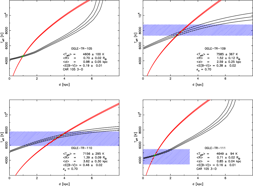
Figure 9: Same as Fig. 7 for OGLE-TR-105, OGLE-TR-109, OGLE-TR-110 and OGLE-TR-111. A colour figure is available in the electronic version of the paper.

Figure 13: $I$ vs $V-I$ colour-magnitude diagram for the CAR 104 and CAR 105 fields. The filled circles are the transit candidates. The lines show the Padova isochrones for solar age and metallicity (corrected for reddening), at distances of 1 kpc (solid line), 2 kpc (dotted line) and 4 kpc (short dashed line). Note that, unlike the field stars, stars with transits have been corrected for reddening and that the most likely transit candidates to host exoplanets are marked with full squares.

Figure 14: $K$ vs $V-K$ colour-magnitude diagram for the CAR104 and CAR105 fields. The filled circles are the transit candidates. The lines show the Padova isochrones for solar age and metallicity (corrected for reddening), at distances of 1 kpc (solid line), 2 kpc (dotted line) and 4 kpc (short dashed line). Note that, unlike the field stars, stars with transits have been corrected for reddening and that the most likely transit candidates to host exoplanets are marked with full squares.

References

- (1) Bertin, E., Arnouts, S., 1996, A&AS 117, 393
- (2) Brown, T M., Charbonneau, D, Gilliland, R. L., Noyes, R. W., Burrows, A., 2001, ApJ 552, 699
- (3) Bonifacio, P., Caffau, E., & Molaro P., 2000, A&A Suppl. Ser. 145, 473
- (4) Bouchy F. et al. 2004, A&A 421, L13
- (5) Bruntt, H. et al. 2003, A&A 410, 323
- (6) Cardelli, J.A., Clayton, G.C., Mathis, J.S., 1989, ApJ 345, 245
- (7) Charbonneau, D., Brown, T. M., Latham, D., Mayor, M., 2000, ApJ 529, L45
- (8) Charbonneau, D., 2003, IAU Symp 219, 152
- (9) Cordes, J.M., Lazio, T.J.W., 2003, ApJ submitted
- (10) Di Benedetto, G. P., 1998, A&A 339, 858
- (11) Drake, A., 2003, ApJ 589, 1020
- (12) Drake A., Cook, K.H. 2004, ApJ 604, 379
- (13) Dreizler, S., Rauch, T., Hauschildt, P., Schuh, S. L., Kley, W., Werner, K., 2002, A&A 391, L17
- (14) Drimmel, R., Cabrera-Lavers, A., López-Corredoira, M., 2003, A&A 409, 205
- (15) Friel, E. D., Janes, K. A., 1993, A&A 267, 75
- (16) Georgelin, Y.M. et al.. 2000, A&A 357, 308
- (17) Girardi, L., Bertelli, G., Bressan, A., Chiosi, C., et al., 2002, A&A 391, 195
- (18) Gonzalez, G., 2003, Rev. Mod. Phys., 75, 101
- (19) Hernandez, X., Valls-Gabaud, D., Gilmore, G., 2000, MNRAS 316, 605
- (20) Horne, K., 2003, in ASP Conf. Ser. 294, eds. D. Deming & S. Seager (San Francisco: ASP), 361
- (21) Kervella, P., Thévenin, F., Di Folco, E. & Ségrasan, D., 2004, A&A in press (astro-ph/0404180)
- (22) Konacki, M., Torres, G., Jha, S., Sasselov, D. D., 2003, Nature 421, 507
- (23) Konacki, M., Torres, G., Sasselov, D. D., Jha, S., 2003, ApJ 597, 1076
- (24) Lineweaver, C.H., Grether, D., 2003, ApJ 598, 1350
- (25) McCarthy C., Zuckerman B., 2004, AJ 127, 2871
- (26) Mendez, R.A., van Altena, W.F., 1998, A&A 330, 910
- (27) Nakanishi H., Sofue, Y. 2003, PASJ 55, 191
- (28) Patriarchi, P., Morbidelli L., & Perinotto M., 2003, A&A 410, 905
- (29) Perryman, M. A. C., Lindegren, L., Kovalevsky, J., et al., 1997, A&A 323, L49
- (30) Pont, F., Bouchy, F., Queloz, D., Santos, N., Melo, C., Mayor, M., Udry, S., 2004, A&A in press. (astro-ph/0408499)
- (31) Ribas, I., Solano, E., Masana, E., Giménez, A., 2003, A&A 411, L501
- (32) Rieke, G. H., Lebofsky, M. J., 1985, ApJ 288, 618
- (33) Robin, A.C., Reylé, C., Derrière, S., Picaud, S., 2003, A&A 409, 523
- (34) Santos, N.C., Israelian, G., Mayor, M., 2004, A&A 415, 1153
- (35) Seager, S., Mallén-Ornelas, G., 2003, ApJ 585, 1038
- (36) Sirko, E., Paczyński, B., 2003, ApJ 592, 1217
- (37) Street, R.A. et al. 2003, MNRAS 340, 1287
- (38) Taylor, J.H., Cordes, J.M., 1993, ApJ 411, 674
- (39) Torres, G., Konacki, M., Sasselov, D., Jha, S., 2004, ApJ in press (astro-ph/0406627)
- (40) Udalski, A., Paczyński, B., Żebruń, K., Szymański, et al., 2002a, Acta Astron. 52, 1
- (41) Udalski, A., Szewczyk, O., Żebruń, K., Pietrzyński, G., Szymański, et al., 2002b, Acta Astron. 52, 317
- (42) Udalski A., 2004, ApJ 590, 284
- (43) Vallenari, A., Bertelli, G., Schmidtobreick, L., 2000, A&A 361, 73
- (44) Wramdemark S. 1980, A&A Suppl Ser. 41, 33