Quantification of discreteness effects in cosmological N-body simulations:
I. Initial Conditions

Abstract

Abstract

The relation between the results of cosmological N-body simulations, and the continuum theoretical models they simulate, is currently not understood in a way which allows a quantification of N dependent effects. In this first of a series of papers on this issue, we consider the quantification of such effects in the initial conditions of such simulations. A general formalism developed in Gabrielli (2004) allows us to write down an exact expression for the power spectrum of the point distributions generated by the standard algorithm for generating such initial conditions. Expanded perturbatively in the amplitude of the input (i.e. theoretical, continuum) power spectrum, we obtain at linear order the input power spectrum, plus two terms which arise from discreteness and contribute at large wavenumbers. For cosmological type power spectra, one obtains as expected, the input spectrum for wavenumbers $k$ smaller than that characteristic of the discreteness. The comparison of real space correlation properties is more subtle because the discreteness corrections are not as strongly localised in real space. For cosmological type spectra the theoretical mass variance in spheres and two point correlation function are well approximated above a finite distance. For typical initial amplitudes this distance is a few times the inter-particle distance, but it diverges as this amplitude (or, equivalently, the initial red-shift of the cosmological simulation) goes to zero, at fixed particle density. We discuss briefly the physical significance of these discreteness terms in the initial conditions, in particular with respect to the definition of the continuum limit of N-body simulations.

today

I Introduction

The goal of dissipationless cosmological N-body simulations (NBS) is to trace the evolution of the clustering of matter under its self-gravity, starting from a cosmological time at which perturbations to homogeneity are small at the physically relevant scales (for reviews, see e.g. Efstathiou et al. (1985); Couchman (1991); Bertschinger (1998)). A fundamental question about such simulations concerns the degree to which they reproduce the evolution of the simulated models. The problem arises because the N-body technique, which simulates a large number of particles evolving under their self-gravity (with some small scale regularization), is not a direct discretization of the theoretical models. The N-body approach is taken because it is not numerically feasible to simulate, at a useful level of resolution, the continuum Vlasov-Poisson equations describing the evolution theoretically.

Since the Vlasov-Poisson system corresponds to an appropriately defined N $\rightarrow\infty$ of this particle dynamics Braun and Hepp (1997); Spohn (1991), NBS can be considered as related to the models in this limit. The problem of discreteness is thus that of the relation of the results obtained from these simulations, for typical statistical quantities characterising clustering, with those which would be obtained with such a simulation done with N $\rightarrow\infty$ particles. The existing studies of this “convergence” problem in the literature (e.g. Efstathiou et al. (1985); Splinter et al. (1998); Melott et al. (1997); Hamana et al. (2002); Diemand et al. (2004a, b)) are almost exclusively numerical, and consider the stability of different measured quantities as a function of N. In the absence, however, of any analytic understanding of the possible N dependence of the results, such studies, which extend over a very modest range of N, cannot be conclusive. Different groups of authors have in fact drawn very different conclusions about the correctness of results for standard quantities at smaller scales. Some Splinter et al. (1998); Melott (1990) even place in question the validity of results for clustering amplitudes below the initial interparticle distance, while such results are widely interpreted as physical in almost all current simulations. Further it is not specified in such studies how precisely the limit of large N should be taken, i.e., which other parameters (e.g. box-size, force softening, initial red-shift) should be kept fixed or varied. These questions are becoming of ever greater practical importance as the quantification of the precision of results from simulations is essential in order to confront cosmological models with a rich host of observations (see, e.g., Huterer and Takada (2005)).

In this paper we address only one simple aspect of this problem: the relation between the discretized initial conditions (IC) of an NBS and the IC of the corresponding theoretical model. More specifically we study and quantify analytically the differences between the two for the two point correlation properties, in real space and reciprocal space, in the infinite volume limit (at a fixed particle density). The discreteness effects, i.e., the differences between the continuous theoretical IC and the discrete IC of the actual NBS are then terms which depend on the particle density. We study these terms and their relative importance for different theoretical IC. We also study and check our analytic results with the aid of numerical simulations, performed in one dimension because of the modest numerical cost of calculating the ensemble average using a large number of realisations. We underline that our analytic results apply to the infinite volume limit, i.e., to the case that the size of the simulation box goes to infinity at fixed particle density. They thus do not include effects associated with the finite size of the box. Such effects, which are quite distinct from those studied here, have been studied extensively elsewhere (see e.g. Gelb and E. Bertschinger (1994); Colombi et al. (1994, 1995, 1996); Pen (1997); Sirko (2005)), both analytically and numerically.

The direct motivation for this work on IC in NBS came originally from some numerical studies of these issues by two groups Baertschiger and Sylos Labini (2002); Dominguez and Knebe (2003); Baertschiger and Sylos Labini (2003); Knebe and Dominguez (2003), who have drawn quite different conclusions about the accuracy with which the IC produced by the canonically used algorithm in NBS represent the input IC . The results in this paper, which are essentially analytic, clarify the issues underlying the discussion in and differences between these numerical studies. Our conclusions are consistent with the findings of both sets of authors, and explain the differences. In short the authors of Dominguez and Knebe (2003); Knebe and Dominguez (2003) are correct that certain real space properties, notably the mass variance in spheres, are in fact reasonably well represented for typical IC in NBS. The authors of Baertschiger and Sylos Labini (2002), however, are correct in diagnosing the important systematic differences between the actual and theoretical correlation properties in real space. Indeed one of our main findings is that there is a very non-trivial difference between the two spaces: while the discreteness of the underlying particle distribution is strictly localized in reciprocal space, this is not the case in real space. The result is that, in the limit of low amplitude initial density fluctuations — or, equivalently, high initial redshift for the simulation — the correlation properties of the input theoretical model are approximated well only in reciprocal space. Taking instead the limit that the particle density goes to infinity at fixed amplitude, the theoretical correlation properties are recovered in both real and reciprocal space, provided an appropriate cut-off is imposed at large wavenumber in the input PS.

The implications of these results for what concerns the agreement between an evolved NBS and the evolved theoretical model of which it is the discretization is beyond the scope of this paper. In a forthcoming paper Joyce and Marcos (2006), treating discreteness effects up to shell crossing, we will see that the evolution of an NBS deviates arbitrarily from its continuum counterpart as the initial red-shift increases at fixed particle density, while keeping the amplitude fixed at increasing particle one approximates increasingly well the continuum (fluid limit) evolution. Thus the results we find for the initial conditions here do indeed turn out to have physical significance for the question of discreteness effects in the evolved simulations.

The algorithm used to generate IC in NBS which we analyze is in fact well defined, in the infinite volume limit, only for a certain range of asymptotic behaviors of the input theoretical PS. We specify here carefully these limits. While it turns out that they are not particularly relevant to current cosmological models, they are of interest in other contexts in which this algorithm may be used, notably in the study of gravitational clustering from other classes of initial conditions (e.g. Melott and Shandarin (1990); Bagla and Padmanabhan (1997)). These properties are also of interest in the context of statistical physics, where the problem of “realizability” of point processes is studied (see e.g. Costin and Lebowitz (2004); Crawford et al. (2003); Uche et al. (2006)). Specifically we find that the algorithm has interesting limits for the case of very “blue” input PS: for the case of spectra with a small $k$ behavior proportional to $k^{n}$, and $n>1$, the real space variance is never that of the input model, while for $n>4$ the reciprocal space representation is never faithful either.

The paper is organized as follows. In the section which follows we briefly review the standard method for setting up IC for cosmological simulations, using the Zeldovich approximation. This also sets conventions for notation in the rest of the paper. In Sect. III we analyze the PS of the configurations of points generated in this way, comparing it with the PS of the input theoretical model. To obtain these results we use a very general exact result derived in Gabrielli (2004), which gives the two point properties of a point distribution generated by superimposing an arbitrary correlated displacement field on an arbitrary initial stochastic point distribution. In the following section we consider how these properties described in $k$-space translate into real space. Specifically we present a general qualitative analysis of the relation between the two point correlation properties of the IC and those of the input models. We treat specifically the mass variance in spheres, and the reduced two point correlation function. For the latter case the comparison of the theoretical model and full IC is more difficult, because of the complicated non-monotonic form of the correlation function of the underlying point distributions. In the following section we illustrate, and verify our results quantitatively, using one dimensional numerical simulations. We choose to work in one dimension for numerical economy, and because all the pertinent questions can be posed equally well and answered in this case. In the final section we summarize our results, discuss what conclusions can be drawn concerning the papers mentioned above which motivated the present study, and finally briefly comment on the physical significance of our results, which will be further developed in the companion paper Joyce and Marcos (2006). Several technical details in the paper, notably concerning the perturbative expansion of the exact expression for the PS of the generated IC, are given in three appendices.

II Generation of IC using the Zeldovich approximation

The method which is used canonically for the generation of IC in cosmological NBS is based on the so-called Zeldovich approximation (ZA)Zeldovich (1970). It may be derived at linear order in a perturbative treatment of the equations describing a self-gravitating fluid in the Lagrangian formulationBuchert (1992). It relates the initial position $\mathbf{q}$ of a fluid element to its final position $\mathbf{x}$ through the expression

$$\mathbf{x}(\mathbf{q},t)=\mathbf{q}+f(t)\mathbf{u}(\mathbf{q})\,,$$ (1)

i.e., it expresses the displacement of a particle as a separable function of the initial position $\mathbf{q}$ and the time $t$. The function $f(t)$ is equal, up to an arbitrary normalization, to the growth factor of density perturbations derived in linear perturbation theory (see below). The vector field $\mathbf{u}(\mathbf{q})$ is thus proportional to both the velocity and acceleration of the fluid element, and with a suitable normalization it can thus be taken to satisfy

$$\mathbf{u}(\mathbf{q})=-\mathbf{\nabla}\cdot\Phi(\mathbf{q})$$ (2)

where $\Phi(\mathbf{q})$ is the gravitational potential at the initial time created by the density fluctuations. To set up IC representing a density field, one thus simply determines the associated potential through the Poisson equation and infers the appropriate displacements [and velocities, given $f(t)$] using Eq. (1) to apply to a set of points representing the unperturbed fluid elements.

We note that to understand this algorithm for generating IC representing a continuous density field it is not in fact necessary to invoke the ZA, nor anything which has specifically to do with gravity. These latter are relevant only for the determination of the velocity field. The only relation needed is in fact the continuity equation, which relates the velocity (and thus displacement) field in a fluid to the density fluctuations. At leading order in the density fluctuations it gives

$$\delta\rho(\mathbf{x})=-\mathbf{\nabla}\cdot\mathbf{u}(\mathbf{x}).$$ (3)

where the density fluctuation $\delta\rho(\mathbf{x})$ is defined by

$$\delta\rho(\mathbf{x})=\frac{\rho({\mathbf{x}})-\rho_{0}}{\rho_{0}},$$ (4)

$\rho(\mathbf{x})$ is the (continuous) density field, $\rho_{0}$ the average density, and $\mathbf{u}(\mathbf{x})$ is the displacement field. By inversion one can determine a displacement field which gives a desired density field. If one assumes further that the former is curl-free, and thus derivable as the gradient of a scalar field, one obtains a unique prescription for the displacement field which is identical to that given by the ZA as described above.

In cosmological models the starting point for IC is not a specific density field, but a power spectrum (PS) of density fluctuations. The latter is defined as

$$P(\mathbf{k})=\lim_{V\to\infty}\frac{\langle{|\delta\hat{\rho}(\mathbf{k})|^{2}}\rangle}{V}\,,$$ (5)

where $\langle\dots\rangle$ denotes the average over an ensemble of realizations and $\hat{\delta}\hat{\rho}(\mathbf{k})$ denotes the Fourier transform (FT) of $\rho(\mathbf{x})$ defined as

$$\delta\hat{\rho}(\mathbf{k})=\int_{V}d^{d}x\delta\rho(\mathbf{x})e^{-i\mathbf{k}\cdot\mathbf{x}}.$$ (6)

It follows then from Eq. (3) that

$$P(\mathbf{k})=k_{i}k_{j}\hat{g}_{ij}(\mathbf{k})$$ (7)

where

$$g_{ij}(\mathbf{k})=\lim_{V\to\infty}\frac{\langle\hat{u}_{i}(\mathbf{k})\hat{u}_{j}^{*}(\mathbf{k})\rangle}{V}$$ (8)

and $\mathbf{\hat{u}}(\mathbf{k})$ is the Fourier transform (FT) of the vector field $\mathbf{u}(\mathbf{q})$. Assuming that the latter is derived from a scalar potential as in Eq. (2) we have

$$\hat{g}_{ij}(\mathbf{k})=\hat{k}_{i}\hat{k}_{j}\hat{g}(k)$$ (9)

where $\hat{g}(\mathbf{k})=Tr[\hat{g}_{ij}(\mathbf{k})]$ is a function of $k=|\mathbf{k}|$ only because the stochastic process is assumed to be statistically homogeneous and isotropic, and $\mathbf{\hat{k}}=\mathbf{k}/|\mathbf{k}|$. We thus have

$$P(\mathbf{k})=k^{2}\hat{g}(k)=k^{4}P_{\Phi}(k)$$ (10)

where $P_{\Phi}(k)$ is the PS of the fluctuations in the scalar field, i.e.,

$$P_{\Phi}(k)=\lim_{V\to\infty}\frac{\langle|\Phi(\mathbf{k})|^{2}\rangle}{V}.$$ (11)

If one considers now a displacement field which varies as a function of time as in Eq. (1), it follows that the PS of density fluctuations is proportional to the square of the function $f(t)$. For a self-gravitating fluid such a behavior applies, and thus one can determine the function $f(t)$ for the determination of the velocities. Indeed Zeldovich originally proposed his approximation as an ansatz, on the basis that Eq. (1) implies the correct evolution of the density fluctuation in linearized Eulerian theory. The power of the ZA is that it can be applied well beyond the regime of validity of Eulerian perturbation theory, to which it matches at early times.

To set up IC for the $N$ particles of a cosmological NBS the procedure is then White (1993); Efstathiou et al. (1985):

• to set-up a “pre-initial” configuration of the $N$ particles. This configuration should represent the fluid of uniform density $\rho_{0}$. The usual choice is a simple lattice, but a commonly used alternative White (1993) is an initial “glassy” configuration obtained by evolving the system with negative gravity (i.e. a Coulomb force) with an appropriate damping.

• given an input theoretical PS $P_{th}(k)$, the corresponding displacement field in the ZA is applied to the “pre-initial” point distribution. The cosmological IC are usually taken to be Gaussian, and the displacements are determined by generating a realization of the gravitational potential

  $$\Phi(\mathbf{q})=\sum_{\mathbf{k}}a_{\mathbf{k}}\cos(\mathbf{k}\cdot\mathbf{q})+b_{\mathbf{k}}\sin(\mathbf{k}\cdot\mathbf{q})$$ (12)

  with

  $$a_{\mathbf{k}}=R_{1}\frac{\sqrt{P_{th}(k)}}{k^{2}},\quad b_{\mathbf{k}}=R_{2}\frac{\sqrt{P_{th}(k)}}{k^{2}}\,,$$ (13)

  where $R_{1}$ and $R_{2}$ are Gaussian random numbers of mean zero and dispersion unity. From Eq. (10) we see that this corresponds to generating a realization of a stochastic displacement field with PS $\hat{g}_{ij}(\mathbf{k})$ as in Eq. (9) and

  $$\hat{g}(k)=P_{th}(k)/k^{2}\,.$$ (14)

III Analytic results in $k$-space

The configuration (or ensemble of configurations) generated by the method outlined in the previous section has PS given through Eq. (10), and thus equal to the theoretical PS $P_{th}(k)$, up to the following approximations:

• The system is considered as a continuous fluid. Thus we expect the exact PS of the (discrete) particle distribution to differ by terms which come from the “granularity” (i.e. particle-like) nature of this distribution.

• The calculations are performed at leading order in the amplitude of the density fluctuations, or equivalently, at leading order in the gradient of the displacements (cf. Eq. (3)). We would thus anticipate that the exact PS of the generated configurations will have corrections which are significant for $k$ larger than the inverse of a scale characterising the amplitude of the input PS.

The rest of the paper is principally focussed on the consideration of the differences arising from the first point between the theoretical PS $P_{th}(k)$ and the exact PS (which we will simply denote $P(\mathbf{k})$) of the distribution generated by the algorithm described in the previous section. We refer the reader to Scoccimarro (1998); Valageas (2002) for analyses of the second point, i.e. of corrections coming from the use of the leading order ZA. These latter studies work in the continuum limit, and so completely decouple the problem of non-linear corrections from the effects of discreteness studied here.

III.1 General results

The starting point for our analysis is a result derived in Gabrielli (2004). One considers, in $d$ dimensions, the application of a displacement field $\mathbf{u}(\mathbf{r})$ to a generic point distribution. The latter is taken to have PS $P_{in}(\mathbf{k})$ and correlation function $\tilde{\xi}_{in}(\mathbf{r})$, given by the inverse Fourier transform

$$\tilde{\xi}_{in}(\mathbf{r})=\frac{1}{(2\pi)^{d}}\int d^{d}k\,e^{-i\mathbf{k}\cdot\mathbf{r}}P_{in}(\mathbf{k}),$$ (15)

where the integral is over all space. The displacement field $\mathbf{u}(\mathbf{r})$ is assumed to be a realization of a continuous stochastic process, which is statistically homogeneous. An exact calculation Gabrielli (2004) gives that the PS of the distribution obtained in this way may be written as

$$P(\mathbf{k})=\int d^{d}re^{-i\mathbf{k}\cdot\mathbf{r}}\hat{p}(\mathbf{k};\mathbf{r})\left(1+\tilde{\xi}_{in}(\mathbf{r})\right)-(2\pi)^{d}\delta(\mathbf{k}).$$ (16)

where

$$\hat{p}(\mathbf{k};\mathbf{r})=\int d^{d}s\,e^{-i\mathbf{k}\cdot\mathbf{s}}p(\mathbf{s};\mathbf{r}),$$ (17)

and $p(\mathbf{s};\mathbf{r})$ is the probability that two particles with a separation $\mathbf{r}$ undergo a relative displacement $\mathbf{s}$.

We note that our choice of notation here follows also that of Schneider and Bartelmann.M. (1995) (rather than that of Gabrielli (2004)). In this work (see also Taylor and Hamilton (1996)) an expression for the PS generated by displacements given by the ZA is derived, for the case of a continuous fluid. The general expression given is exactly that obtained by setting $\tilde{\xi}_{in}(\mathbf{r})=0$ in (16). This extra term in our expression arises because we do not make the approximation of treating the “pre-initial” configuration as a continuous uniform background. We note that this additional term contains not just the effect of taking into account the correlations in the “pre-initial” configuration, but also includes more generally all the effects of the discreteness of the (“pre-initial” and final) distribution. In this respect we note that the correlation function $\tilde{\xi}_{in}(\mathbf{r})$ for the “pre-initial” distribution contains generically a delta-function at $r=0$, which is characteristic of its discreteness, as well as a non-singular function which describes correlations (for a detailed discussion see Gabrielli et al. (2004a); Gabrielli et al. (2002)).

From the definition of $p(\mathbf{s},\mathbf{r})$ it follows that

$$\hat{p}(\mathbf{k},\mathbf{r})=\int{\cal D}\mathbf{u}\,{\cal P}(\{\mathbf{u}({\mathbf{r}})\})\,e^{-i\mathbf{k}\cdot[\mathbf{u}(\mathbf{r})-\mathbf{u}(\mathbf{0})]}$$ (18)

where the functional integral is over all possible displacement fields weighted by their probability ${\cal P}(\{\mathbf{u}(\mathbf{r})\})$. For a displacement field which is (i) Gaussian, and (ii) statistically isotropic (as well as homogeneous) it is then simple to show Gabrielli (2004) that

$$\hat{p}(\mathbf{k},\mathbf{r})=e^{-k_{i}k_{j}d_{ij}(\mathbf{r})}$$ (19)

where a sum is implied over the labels $i$ and $j$, and

$$d_{ij}(\mathbf{r})\equiv g_{ij}(0)-g_{ij}(\mathbf{r})\,,$$ (20)

where

$$g_{ij}(\mathbf{r})=\langle u_{i}(0)u_{j}(\mathbf{r})\rangle$$ (21)

is the (matrix) two-displacement correlation function. We note that the scalar function

$$g(r)=Tr(g_{ij}(\mathbf{r}))=\langle\mathbf{u}(0)\cdot\mathbf{u}(\mathbf{r})\rangle$$ (22)

is simply the inverse FT of $\hat{g}(k)$ defined above (and, by statistical isotropy, a function only of $r=|\mathbf{r}|$), and that $g(0)=\langle u^{2}\rangle$ is the variance of the displacement field. We have that

$$d_{ij}(\mathbf{r})=\frac{1}{2}\langle\left[u_{i}(0)-u_{i}({\mathbf{r}})\right]\left[u_{j}(0)-u_{j}({\mathbf{r}})\right]\rangle\,,$$ (23)

i.e., it is proportional to the correlation matrix of the relative displacements.

Substituting (19) in (16), we obtain

$$P(\mathbf{k}) = \int_{\Omega}d^{d}re^{-i\mathbf{k}\mathbf{r}}e^{-k_{i}k_{j}d_{ij}(\mathbf{r})}\left(1+\tilde{\xi}_{in}(\mathbf{r})\right)$$ (24)

$$- (2\pi)^{d}\delta(\mathbf{k}).$$

It will be useful for our discussion to break this expression into two pieces, $P(\mathbf{k})=P_{\rm c}(\mathbf{k})+P_{\rm d}(\mathbf{k})$, written in the form

$$P_{\rm c}(\mathbf{k}) =\int_{\Omega}d^{d}re^{-i\mathbf{k}\mathbf{r}}\left(e^{-k_{i}k_{j}d_{ij}(\mathbf{r})}-1\right)$$ (25a)

$$P_{\rm d}(\mathbf{k}) =P_{\rm in}(\mathbf{k})+\int_{\Omega}d^{d}re^{-i\mathbf{k}\mathbf{r}}\left(e^{-k_{i}k_{j}d_{ij}(\mathbf{r})}-1\right)\tilde{\xi}_{in}(\mathbf{r})\,.$$

The first term Eq. (25a) is the “continuous” piece of the generated PS (identical, as discussed above to that given in Schneider and Bartelmann.M. (1995)), and the second term Eq. (25) is the contribution coming from the discreteness.

III.2 Application to cosmological IC

In the algorithm used to generate cosmological NBS, we have seen that the FT of $g_{ij}({\mathbf{r}})$ is [cf. Eqs. (9) and (14)] given by

$$\hat{g}_{ij}(\mathbf{k})=\hat{k}_{i}\hat{k}_{j}\frac{P_{\rm th}(k)}{k^{2}}\,.$$ (26)

Expanding the exponential factor in Eq. (25a) and (25) in power series, we can thus obtain expressions for $P_{\rm c}(\mathbf{k})$ and $P_{\rm d}(\mathbf{k})$ at each order in powers of $P_{\rm th}(k)$. At zero order we have evidently

$$P^{(0)}_{\rm c}(\mathbf{k})=0\qquad P^{(0)}_{\rm d}(\mathbf{k})=P_{\rm in}(\mathbf{k})$$ (27)

and, at linear order,

$$P^{(1)}_{\rm c}(k)=P_{\rm th}(k)$$ (28a)

$$P^{(1)}_{\rm d}(k)=\frac{k^{2}}{(2\pi)^{d}}\int_{\Omega}d^{d}q (\mathbf{\hat{k}}\cdot\mathbf{\hat{q}})^{2}\frac{P_{th}(q)}{q^{2}}$$

$$\times[P_{in}(\mathbf{k}+\mathbf{q})-P_{in}(\mathbf{k})]$$ (28b)

To this order the PS of the generated distribution is thus the sum of the input theoretical PS and two discreteness terms: the PS of the “pre-initial” (i.e. lattice or glass) distribution and a second term which is a convolution of the input PS and the “pre-initial” PS. At next order in the expansion (i.e. at second order in $P_{\rm th}(k)$) we will obtain both further discreteness corrections, and corrections which survive in the limit in which we neglect discreteness completely. This result is in line with what we anticipated at the beginning of this section.

III.3 Domain of validity of the expansion

We have implicitly assumed above that the expansion we have performed is well defined . This assumption corresponds to that of finiteness of various integrals of the input PS $P_{\rm th}(k)$. If the latter function is well-behaved, this corresponds to constraints on its asymptotic properties, at small and large $k$. To determine these constraints we consider a PS of the form

$$P_{th}(k)=Ak^{n}f(k/k_{c})$$ (29)

where $A$ and $n$ are constants, and $f(x)$ is a function which interpolates between unity for $x\ll 1$ and zero for $x\gg 1$, i.e., which may act as a cut-off for $k>k_{c}$. In the use of this algorithm in cosmological simulations, for reasons which we will discuss further below, a very abrupt (usually top-hat) such cut-off is always imposed at wavenumbers of order the inverse of the scale characteristic of the interparticle separation . Thus we will consider only the constraints at small $k$, i.e., the lower bound placed on the index $n$.

Firstly we note that, using Eqs. (20) and  (26), it is simple to show that $d_{ij}({\bf r})$ is well defined only if

$$\lim_{k\rightarrow 0}k^{d}P_{th}(k)=0\,,$$ (30)

i.e., if $n>-d$ in Eq. (29). This is a condition which is always satisfied in cosmological models, as it follows from the finiteness of the one-point variance of the theoretical density fluctuations .

In App. A we analyse in detail the full expansion of $P_{c}(k)$ to all orders in $A$, separating two different cases: (i) $-d<n<-d+2$, in which the one point variance $g(0)$ is infinite, and (ii) $n>-d+2$, in which case $g(0)$ is finite. From the expansions in each case one can infer the following:

• For $-d<n<-d+2$ the leading non-zero term, equal to $P_{th}(k)$, approximates well the full $P_{\rm c}(\mathbf{k})$ for the range of $k$ in which

  $$\Delta_{\rm th}^{2}(k)\equiv k^{d}P_{th}(k)\ll 1\,.$$ (31)

• For $-d+2<n<4$ the criterion to satisfy the same condition is:

  $$k^{2}g(0)=k^{2}\langle u^{2}\rangle\ll 1\,.$$ (32)

• For $n\geq(-d+2)+d/2$ there is, at next order in the expansion of $P_{\rm c}(k)$, a correction proportional to $k^{4}$. This implies that, for $n\geq 4$ the leading term $P_{th}(k)$ is never well approximated at asymptotically small $k$ by the PS of the generated IC.

To analyse the expansion of the discreteness contribution $P_{\rm d}(\mathbf{k})$ we need to specify the “pre-initial” distribution. It is evident however that generically it is at least as convergent as than that of $P_{c}(k)$, since Eq. (25) contains in the integrand simply an extra factor of $\tilde{\xi}_{in}(\mathbf{r})$, which is typically smaller than unity and decreasing at large separations. For a Poisson distribution of number density $n_{0}$, for example, one has $\tilde{\xi}_{in}(\mathbf{r})=\frac{1}{n_{0}}\delta(\mathbf{r})$ (where $\delta(\mathbf{r})$ is a Dirac delta function in $d$-dimensions), and therefore the expansion becomes trivial with $P_{\rm d}(k)=P_{\rm in}(k)=\frac{1}{n_{0}}$ at all orders. In cosmological NBS the “pre-initial” distribution, as we have discussed, is usually taken to be a simple lattice or glass. We will see below that for the case of the lattice the coefficients of the expansion are sums which are regulated at small $k$, by the Nyquist frequency of the lattice (defined below). For the case of the glass, or indeed any distribution with an analytic $P_{\rm in}(\mathbf{k})$, we limit ourselves to an analysis of the integral coefficient of the leading term in Eq. (28b). It is simple to see, by Taylor expanding the expression inside the square brackets at small $q$, that the finiteness requires only the integrability of $P_{\rm th}(q)$ at small $q$. This coincides precisely with the condition Eq. (30). We expect that $P_{\rm d}(\mathbf{k})\approx P^{(0)}_{\rm d}(\mathbf{k})+P^{(1)}_{\rm d}(\mathbf{k})$ will thus also be satisfied when Eq. (31) applies. We will verify below with numerical simulations that this is indeed the case.

We note that the condition Eq. (31) for the validity of the perturbative expansion at a given $k$ is one which could be guessed from the simple continuum derivation using Eq. (3), in which the expansion parameter is the amplitude of the theoretical density fluctuation: $\Delta_{\rm th}^{2}(k)$ is just a dimensionless measure of the amplitude of the density fluctuations in the theoretical model arising from wavenumbers around $k$ . Further we show in App. A that if condition Eq. (32) is fulfilled for any $k<k_{c}$, then Eq. (31) is also. The two conditions are in fact essentially equivalent in the case that a cut-off is imposed as typically is done the cosmology.

III.4 The leading non-trivial discreteness correction

Let us now analyse in more detail the leading contribution to the generated PS arising from discreteness, i.e., the expression which we have denoted above by $P_{\rm d}^{(1)}(\mathbf{k})$ . We note [cf. Eqs. (28a-28b)] that this term arises at the same order as the input PS in the perturbative expansion, i.e., at linear order in the amplitude of the input theoretical PS. We consider the specific case of a “pre-initial” distribution which is a simple cubic lattice. Its PS is

$$P_{in}(\mathbf{k})=(2\pi)^{d}\sum_{\mathbf{h}\neq 0}\delta(\mathbf{k}-\mathbf{h})$$ (33)

where the sum over $\mathbf{h}$ is over all the vectors of the reciprocal lattice, i.e., $\mathbf{h}=\mathbf{m}(2\pi/\ell)$, where $\ell$ is the lattice spacing and $\mathbf{m}$ is a vector of non-zero integers. The minimal value of $|\mathbf{h}|=2\pi/\ell$, is the sampling frequency $k_{s}$ of the lattice, equal to twice the Nyquist frequency, which we will denote $k_{N}$ (and $k_{N}=\pi/\ell$). It is instructive to rewrite the first order term Eq. (28b) in the form

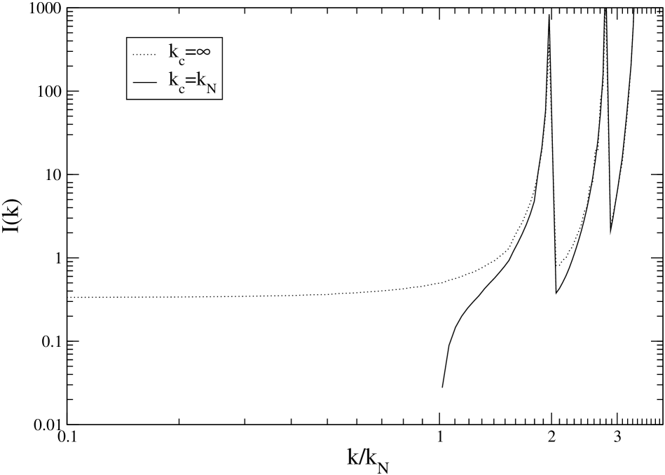
Figure 1: Integral $I(\mathbf{k})$ of Eq. (37), in three dimensions and averaged over shells of $|\mathbf{k}|$, for an input PS $P_{th}(k)$ as in Eq. (29) with $n=-2$ and (i) $f(k)=1$, i.e., without a cut-off (dotted line), and (ii) $f(k)=\Theta(k_{N}-k)$, i.e., an abrupt (Heaviside step function) cut-off at $k=k_{N}$ (solid line). In the former case we see that $I(\mathbf{k})$ is approximately constant for $k<k_{N}$, and therefore the leading discreteness term $P_{d}^{(1)}(k)\sim k^{2}$ for $k<k_{N}$. In the latter case, the discreteness term contributes only for $k>k_{N}$. Such a cut-off is usually employed in the use of this algorithm in cosmological simulations.

$$P_{\rm d}^{(1)}(k)=Ak^{2}k_{N}^{n-2}I(\mathbf{k})$$ (34)

where

$$I(\mathbf{k})\equiv\frac{1}{(2\pi)^{d}}\int{d^{d}q}(\mathbf{\hat{k}}\cdot\mathbf{\hat{q}})^{2}\left(\frac{q}{k_{N}}\right)^{n-2}f(q/k_{c})$$

$$\times[P_{in}(\mathbf{k}+\mathbf{q})-P_{in}(\mathbf{k})]$$ (35)

is dimensionless. Since $P_{in}(\mathbf{k})=0$ for $\mathbf{k}\neq\mathbf{h}$, we therefore have, at linear order in our expansion in powers of the input PS, that,

$$P(\mathbf{k}) = P_{\rm th}(k)+P^{(1)}_{d}(\mathbf{k})$$ (36)

$$= Ak^{n}f(k/k_{c})+Ak^{2}k_{N}^{n-2}I(\mathbf{k})$$

where

$$I(\mathbf{k})=\sum_{\mathbf{h}\neq\mathbf{0}}\frac{[\mathbf{\hat{k}}\cdot(\mathbf{h}-\mathbf{k})]^{2}}{|\mathbf{h}-\mathbf{k}|^{2}}\left(\frac{|\mathbf{h}-\mathbf{k}|}{k_{N}}\right)^{n-2}f(\frac{|\mathbf{h}-\mathbf{k}|}{k_{c}})$$ (37)

for $\mathbf{k}\neq\mathbf{h}$.

Figure 2: As in previous figure, but now for $n=0$ and a top-hat cut-off function, for three different values of the cut-off. We see that as the cut-off increases the amplitude of $I(k)$ does so (corresponding to the UV divergence of the sum Eq. (37) for $n>-1$ in three dimensions). We see again that for a cut-off at $k_{N}$ the leading order discreteness term contributes only for $k>k_{N}$, while for larger cut-off we have aliasing effects which manifest themselves in the appearance of the term $P_{d}^{(1)}(k)\sim k^{2}$ for $k<k_{N}$.

The second (discreteness) term in Eq. (36) includes explicitly what is known as “aliasing”: power in the input spectrum at large wavenumbers (i.e. above the sampling frequency) gives rise to power at small $k$. Indeed the amplitude at small $k$ of the discreteness term is proportional to $I(\mathbf{k}\rightarrow 0)$ in Eq. (35), which is a sum depending strictly on the power in modes at wave-numbers greater than or equal to the sampling frequency $k_{s}=2k_{N}$. Further if one cuts at the Nyquist frequency $k_{N}$, i.e., $f(k/k_{c})=\Theta(k_{N}-k)$, where $\Theta$ is the Heaviside step function, it follows that $I(\mathbf{k})=0$ for $k<k_{N}$. In this case therefore we have, for $\mathbf{k}\neq\mathbf{h}$, that

$$P(\mathbf{k})=P_{\rm th}(k)\Theta(k_{N}-k)+P^{(1)}_{d}(\mathbf{k})\Theta(k-k_{N}),$$ (38)

i.e., to leading order in the input spectrum the full PS of the generated IC is exactly equal to this input spectrum below the Nyquist frequency, and given by the discreteness term Eq. (35) above the Nyquist frequency. It is easy to verify that an analogous result applies if the cut-off is imposed in the first Brillouin zone (FBZ), i.e., setting the PS to zero but for vectors with all three components $\in[-k_{N},k_{N}]$. In cosmological simulations a cut-off is usually imposed in this way (see e.g. Couchman (1991), Bertschinger ).

In Fig. 1 is shown the numerically computed value of $I(\mathbf{k})$ as a function of $k$, in three dimensions, for a pure power-law PS with $n=-2$, (i) without a cut-off [i.e. with $f(k)=1$ in Eq. (29)] and, (ii) with an abrupt top-hat cut-off at $k_{N}$, i.e., $f(k)=\Theta(k_{N}-k)$. In Fig. 2 we show the same quantity but for $n=0$ and three top-hat cut-offs at $k_{N}$, $2k_{N}$, $3k_{N}$. We see clearly illustrated the behaviors discussed above. Note that for $n<-d+2$ ($n>-d+2$) the expression for $I(\mathbf{k})$ converges (diverges) without a cut-off, which explains the choices for the cut-off functions in the two figures. If a sharp cut-off is not implemented at $k_{N}$ we see that, in all cases, $I(\mathbf{k})$ is non-zero and approximately constant for $k<k_{N}$. There is thus an associated aliasing term which is, to a very good approximation, proportional to $k^{2}$.

III.5 Accuracy of generation algorithm in $k$ space

We can now draw clear conclusions about the accuracy with which the generation algorithm, applied on a simple lattice, produces a point distribution with a PS approximating the input PS of the form assumed in Eq. (29):

• For $-d<n<4$, and $f$ an abrupt cut-off at $k_{N}$, we have $P(k)=P_{th}(k)$ for $k<k_{N}$, up to corrections which depend parametrically on the dimensionless quantity $\Delta_{\rm th}^{2}(k)=k^{d}P_{\rm th}(k)$. For $k>k_{N}$ we have $P(k)=P_{\rm d}^{(1)}(k)$, where the latter is a discreteness term given explicitly in Eq. (35).

• If any input power is included above the Nyquist frequency $k_{N}$ of the lattice (or, more precisely, outside the FBZ of the reciprocal lattice), it leads to the appearance of power in the IC at $k<k_{N}$ (i.e. inside the first FBZ). With power included above the sampling frequency ($k=2k_{N}$) there is an aliasing term proportional to $k^{2}$ at small $k$. In this case therefore the range of $n$ which may be accurately represented at small $k$ is limited to $-d<n<2$.

• For $n>4$ one always has $P(k)\propto k^{4}$ at sufficiently small $k$, and the PS of the point process produced by the algorithm therefore does not approximate the input theoretical spectrum.

• For $n<-d$ the algorithm is not well defined because the correlation function of relative displacements $d_{ij}(\mathbf{r})$ is undefined. This is true in the infinite volume limit. In practice one generates IC in a finite system, usually taken to be a cube (with periodic boundary conditions). This means that in practice the input PS is always cut at the corresponding fundamental frequency of the box, so that, even for $n<-d$, the algorithm can be applied. The implication of our result is that one will find in this case that the PS obtained will depend on this box size, becoming badly defined in the infinite volume limit. We will verify that this is the case in our numerical study below.

III.6 Glass pre-initial conditions

The above conclusions were derived assuming that the “pre-initial” distribution is a simple lattice. The alternative starting point quite often used in cosmological NBS are “glassy” configurations, obtained by evolving gravity with a negative sign and a strong damping on the velocities White (1993); Bertschinger . Without the damping, this system is essentially just what is known as the “one component plasma” in statistical physics (for a review, see Baus and Hansen (1980)). The small $k$ behavior of the power spectrum is then expected to be $P_{in}(k)\sim k^{2}$ at small $k$ . With the damping term what is found is a PS with a behavior $\sim k^{4}$ at small scales Smith et al. (2003). Assuming this form for the spectrum it is easy to follow through the analysis given above for this case. The only change is that the term $I(\mathbf{k})$ is now non-zero for all $k$ : because $P_{in}(k)$ is non-zero for all $k$ it is not possible to have zero overlap of its support with that of $P_{\rm th}(k)$ in Eq. (28b). This is what permitted this term to be zero in the case of a lattice and a top-hat cut-off at the Nyquist frequency. Thus in the case of a glass there will generically be a correction $\propto k^{2}$ at $k$ below the wave-number characteristic of the inter-particle distance in the glass. Thus the range of power-law spectra which may be accurately represented by the generation algorithm in this case at small $k$ is $-d<n<2$. The models simulated in the context of cosmological N-body simulations are always well inside this range.

What is the source of these limits on the representation of PS with $n>2$ (or $n>4$ on the lattice)? We remark that the appearance of such terms would appear to be related to a well-known argument used by Zeldovich Zeldovich (1965); Zeldovich and Novikov (1983) in determining the limits imposed by causality on fluctuations (See Peebles (1993) and Gabrielli et al. (2004b) for discussion of this result and further references.): any stochastic process which moves matter in a manner which is correlated only up to a finite scale generates terms proportional to $k^{2}$ in the PS at small $k$. The coefficient of the $k^{2}$ term vanishes, leaving a leading term proportional to $k^{4}$, if the additional condition is satisfied that the center of mass of the matter distribution is conserved (i.e. not displaced) locally . The condition on the support of the displacement field required to make the coefficient of the $k^{2}$ vanish should thus be equivalent to a condition of local center-of-mass conservation under the effect of the displacement field.

IV Results in real space

We now turn to the consideration of the real space properties of the distributions generated by the algorithm. In this section we use the $k$ space results of the previous section to determine these properties approximately, but analytically. In the next section we will use numerical simulations in one dimension to show in detail the validity of these results.

IV.1 Definitions and background

The quantities we will study in real space are the reduced 2-point correlation function $\tilde{\xi}(\mathbf{r})$ and the variance of mass in spheres. In fact we will principally consider the latter for reasons which we will explain below.

We recall that $\tilde{\xi}(\mathbf{r})$, for a statistically homogeneous distribution, is defined by

$$\langle\overline{\rho(\mathbf{r})\rho(\mathbf{r}^{\prime})}\rangle=\rho_{0}^{2}(1+\tilde{\xi}(\mathbf{r}-\mathbf{r}^{\prime})),$$ (39)

where $\langle...\rangle$ is the ensemble average. For a discrete distribution (i.e. the case we always consider here) $\langle\overline{\rho(\mathbf{r})\rho(\mathbf{r}^{\prime})}\rangle dV_{1}\,dV_{2}$ is the a priori probability to find 2 particles in the infinitesimal volumes $dV_{1}$, $dV_{2}$ respectively around $\mathbf{r}_{1}$ and $\mathbf{r}_{2}$. The correlation function $\tilde{\xi}(\mathbf{r})$ measures therefore the deviation of this probability from that in a Poisson distribution (equal to $\langle\rho_{0}\rangle^{2}dV_{1}\,dV_{2}$). It is related to the PS as its Fourier transform.

The normalized mass variance $\sigma^{2}(R)$ in spheres of radius $R$ is defined as

$$\sigma^{2}(R)=\frac{\langle M(R)^{2}\rangle-\langle M(R)\rangle^{2}}{\langle M(R)\rangle^{2}}.$$ (40)

where $M(R)$ is the mass in a sphere of radius R, centered at a randomly chosen point in space. It is given in terms of the correlation function by

$$\sigma^{2}(R)=\frac{1}{V(R)}\int_{V(R)}d^{d}r_{1}\int_{V(R)}d^{d}r_{2}\tilde{\xi}(|\mathbf{r}_{1}-\mathbf{r}_{2}|)$$ (41)

(where $V(R)$ is the volume of a sphere of radius $R$), and in terms of the PS by

$$\sigma^{2}(R)=\frac{1}{(2\pi)^{d}}\int d^{d}kP(\mathbf{k})|\tilde{W}_{R}(k)|^{2}$$ (42)

where $\tilde{W}_{R}(k)$ is the Fourier transform of the window function for a sphere of radius $R$, normalized so that $\tilde{W}_{R}(0)=1$.

It is simple to show (see e.g. Peebles (1993), and Gabrielli et al. (2002); Gabrielli et al. (2004a) for a more detailed discussion) that, for a PS of the form (29), the behavior of the integral in (42) depends strongly on the value of $n$:

• for $-d<n<1$ the integral for $\sigma^{2}(R)$ is dominated by modes $k\sim 1/R$ and one has

  $$\sigma^{2}(R)\sim k^{d}P(k)|_{k\sim 1/R}\propto\frac{1}{R^{d+n}}$$ (43)

• for $n>1$ the integral is dominated by modes $k\sim k_{c}^{-1}$ (i.e. by the ultra-violet cut-off) and one has always

  $$\sigma^{2}(R)\propto\frac{1}{R^{d+1}}.$$ (44)

For $n=1$ one obtains the transition behavior, in which the integral depends logarithmically on the cut-off $k_{c}$. This gives $\sigma^{2}(R)\propto\ln R/R^{d+1}$.

The behavior in Eq. (44) is thus actually a limiting behavior. It is in fact a special case of a much more general result (see Gabrielli et al. (2002); Gabrielli et al. (2004a) for a discussion and references to the mathematical demonstration of this result): the most rapid possible decay in any mass distribution of the unnormalized variance of the mass $\langle(\Delta M)^{2}\rangle_{V}$ in a volume $V$ is proportional to the surface of the volume.

IV.2 Perturbative results in real space

Returning now to Eqs. (27- 28b), and using Eq.(42), we infer that, at linear order in the amplitude of the input PS, we have

$$\sigma^{2}(R) = \sigma_{in}^{2}(R)+\sigma_{th}^{2}(R)+\sigma_{d}^{2}(R)$$ (45)

$$\tilde{\xi}(\mathbf{r}) = \tilde{\xi}_{in}(\mathbf{r})+\tilde{\xi}_{th}(r)+\tilde{\xi}_{d}(\mathbf{r})$$ (46)

for the normalized mass variance and correlation function of the IC. The ‘in’ and ‘th’ subscripts in each case have the obvious meanings, with ‘d’ indicating the term associated to the linear order discreteness correction $P_{d}^{(1)}(k)$. We have assumed implicitly that the integrals pick up negligible contribution from the regions, at large $k$, where the linear approximation to the full PS is not good. This will typically translate into a lower bound on $R$ and $r$ for the validity of Eqs. (45) and (46).

It is simple to understand from Eqs. (45) and (46) why the question of the representation of real space properties of the IC generated using the ZA is non-trivially different from that of $k$ space properties. In $k$ space we had analogous expressions to Eqs. (45) and (46), from which it followed that $P(\mathbf{k})\approx P_{th}(k)$ to very good accuracy at small $k$. One necessary ingredient for this was that the term $P_{in}(k)$ could be neglected at small $k$, as it is identically zero outside the FBZ on a lattice and decreasing very rapidly to zero ($\propto k^{4}$) in a glass. In real space we do not have the same “localization” at large $k$ of the intrinsic fluctuations associated with the pre-initial distribution. Indeed we have noted above that there is a limiting behavior ($\propto 1/R^{d+1}$) to the decay with radius $R$ of the mass variance, for any distribution . The amplitude of this leading term is fixed by the inter-particle distance $\ell$, with $\sigma_{\rm in}^{2}\sim(\ell/R)^{d+1}$, while that of the two other terms Eqs. (45) is proportional to the amplitude $A$ of the input spectrum. Likewise for the correlation function the intrinsic term $\tilde{\xi}_{in}(r)$ is generically delocalised in space, and depends only on the particle density, while the other two terms are proportional to the amplitude of the input PS. At sufficiently low amplitude, both quantities will be dominated at any finite scale by those of the underlying pre-initial point distribution, and thus will not be approximated by their behaviors in the input model. This is a behavior which is qualitatively different to what we have seen in reciprocal space. We now examine in a little more detail these two-point quantities. We treat them separately as they are quite different for what concerns their comparison to the continuous theoretical input quantities: being an integrated quantity, the mass variance is intrinsically smooth and can be directly compared with its counterpart in the input model.

IV.3 Mass variance in spheres

Given Eq. (45), and the limits we have discussed on the behavior of the variance, we can immediately make a simple classification of the PS of the form (29) for what concerns the representation of their variance in real space. The faithfulness of such a representation requires simply

$$\sigma_{th}^{2}(R)\gg\sigma_{in}^{2}(R).$$ (47)

For either a lattice or glass we have the “optimal” decay $\sigma_{in}^{2}(R)\propto 1/R^{d+1}$. In order for Eqs. (45) and (46) to be valid we require that Eqs. (27- 28b) be valid. As discussed in the previous section we expect this to correspond to the criterion that $\Delta_{\rm th}^{2}(k)=k^{d}P_{th}(k)<1$ for the relevant $k$. Given that $P_{d}^{(1)}(k)$ is at most proportional to $k^{2}$ at small $k$, the associated variance is also $\propto 1/R^{d+1}$ above the interparticle distance $\ell$, and thus sub-dominant with respect to the leading term at all scales. Since we generically cut the input spectrum around $k_{N}$, and will consider simple power law spectra up to this scale with $n<-d$, it suffices to have

$$\Delta_{\rm N}^{2}\equiv\Delta_{\rm th}^{2}(k_{\rm N})=k_{\rm N}^{d}P_{th}(k_{\rm N})<1\,.$$ (48)

Up to a numerical factor of order unity this is none other that the criterion that $\sigma_{th}^{2}(\ell)<1$, and so it follows that we expect the following behaviors:

1. For $n>1$ we have seen that $\sigma_{th}^{2}(R)\sim 1/R^{d+1}$, i.e., $\sigma_{th}^{2}(R)$ has the same functional behavior as that of the “pre-initial” variance. Given that the former is necessarily smaller at the inter-particle distance, the condition Eq. (47) will never be fulfilled, as the full variance will be dominated by that of the pre-initial configuration.

2. For $-d<n<1$ we have that $\sigma_{th}^{2}(R)\sim 1/R^{d+n}$, which thus decays more slowly than the “pre-initial” term. Thus there will be a scale $R_{min}$ such that for $R>R_{min}$ one can satisfy the condition Eq. (47). It is easy to infer that, for any $d$, we have

   $$R_{min}\sim\ell\left(\frac{1}{\Delta_{\rm N}}\right)^{\frac{2}{1-n}}$$ (49)

IV.4 Two point correlation function

The case of the two point correlation function is similar. The determination of the range of faithful representation of the theoretical correlation function is, however, more complicated by the very non-monotonic behavior of the correlation function in both the (unperturbed) lattice and glass. This leads, as we will explain, to a strong dependence on how the correlation function is smoothed when it is estimated in a sample.

Unlike for the variance, there is no intrinsic limit on the rapidity of the decay of the correlation function for point processes. Indeed for a Poisson process one has $\tilde{\xi}_{in}(r)=0$ for $r>0$, and exponentially decaying correlation functions are commonplace in many physical systems. For both a lattice and glass distributions the leading term $\tilde{\xi}_{in}(r)$ in Eq. (46) presents a very non-trivial behavior. The two point correlation function of the lattice is in fact not a function of $r$, but a distribution which depends on $\mathbf{r}$: it is proportional to a Dirac delta function when $\mathbf{r}$ links any two lattice points, and equal to $-1$ otherwise (see Appendix C for the explicit expression). For the glass the correlation function is not known exactly — it depends on the details of the generation of the glass configuration used — but generically it will be expected to have a similar oscillatory structure describing its very ordered nature, with decay only at scales considerably above the interparticle distance . This underlying highly ordered structure is evidently not washed out by the application of very small displacements. In particular for relative displacements much smaller than the initial interparticle separation, it is clear that the form of the underlying correlation function will remain highly oscillatory up to a scale considerably larger than the interparticle distance. Just as in the case of the mass variance, therefore, one can conclude that the theoretical term in Eq. (46) will always be dominated by the discreteness terms up to some scale, which becomes larger as the input amplitude is decreased.

A simple analytical estimate, like that given above for the variance, of the scale at which the theoretical term will dominate the discreteness terms, and thus at which the input theoretical two-point correlation function is well approximated by that of the generated IC, is not possible: for the lattice such an estimate must take also into account the term $\tilde{\xi}_{d}(\mathbf{r})$ which together with $\tilde{\xi}_{in}(\mathbf{r})$ gives a regular oscillating and decaying function; for a glass we do not have the analytical form of the correlation function.

There is a further important difficulty if one wishes to compare the correlation function in generated IC with the input one. In estimating the correlation function in a finite sample one must introduce a finite smoothing: one computes it by counting the number of pairs of points with separations in some finite interval, typically a radial shell of some chosen thickness. Indeed while the full correlation function is in general a function of $\mathbf{r}$, this procedure makes it a function of $r$ like the theoretical correlation function. Given that, at low amplitude of the relative displacements, $\tilde{\xi}(\mathbf{r})$ has both a strongly oscillating and strongly orientation dependent behavior, such a smoothing can change very significantly its behavior. Thus the scale at which agreement may be observed between the measured ensemble averaged two point correlation function and that of the input model will depend both on $A$, $\ell$ and the precise algorithm of estimation of the correlation function.

V Numerical study in one dimension

In this section we study the generation algorithm using numerical simulations. This allows us to verify our conclusions about two point properties in reciprocal and real space, derived in the limit of small amplitudes of the input PS. Further it allows it to show the accuracy of the full analytic expression Eq. (24), for any input amplitude. We work in one dimension because of the numerical feasibility of the study in this case: we measure directly the real-space mass variance for a large ensemble of configurations, which is not numerically feasible (for modest computational power) in three dimensions. The exact ensemble average results given above, on the other hand, are easily calculated. The simplified and more explicit expressions for the relevant quantities are given in Appendix C. There is no intrinsic difference of importance between one and three dimensions for the questions we address.

We consider the case in which the pre-initial distribution is a lattice. Following our discussion in the previous sections we study separately the four following specific examples for input PS as in Eq. (29): (i) n=-1/2 (example of $-d<n<1$), (ii) n=3 (example of $1<n<4$), (iii) n=7 (example of $n>4$) and (iv) n=-2 (example of $n<-d$, in which case we have found the algorithm to be badly defined in the infinite volume limit). We will specify the cut-off function in each case. We then also present numerical results for the two point correlation function in just the first of these models to illustrate the discussion of this quantity given at the end of the preceding section.

V.1 $n=-1/2$ (Case $-d<n<1$)

Figure 3: PS of a model with $n=-1/2$, sharp cut-off $f(k)=\Theta(k-k_{N})$ and $\Delta_{N}=1.77\times 10^{-3}$ ($A=10^{-3}$). The simulation results are averaged over one thousand realisations of IC, generated using the standard algorithm (adapted to one dimension).

Figure 4: PS of a model with $n=-1/2$, continuous cut-off $f(k)=\exp(-k/2k_{N})$ and $\Delta_{N}=1.77\times 10^{-3}$ ($A=10^{-3}$).

In Fig. 3 are shown results for an input PS $P_{th}(k)=Ak^{-1/2}$ with $A=10^{-3}$, which corresponds to $\Delta_{N}=1.77\times 10^{-3}$. Here, as in the rest of this section, we use units of length in which the inter-particle distance is equal to unity. We have imposed a sharp FBZ cut-off $f(k)=\Theta(k-k_{N})$. In the figure we see, as expected, excellent agreement between the PS measured by averaging over a thousand realisations of IC, generated using the standard algorithm (with Gaussian displacements) in a periodic interval containing a thousand particles, and the theoretical expression at linear order, as given in the previous section. Note that on the $x-axis$ is given $k/2k_{N}$, so that first Bragg peak appears at unity, and the sharp change in the PS at $0.5$.

Fig. 4 differs only in that we have now imposed a continuous cut-off $f=e^{-k/2k_{N}}$. Again we observe, as expected, excellent agreement between the measured PS and the theoretical expression. The agreement between the input PS and the measured PS is, however, less perfect around $k_{N}$, because the discreteness term $P_{d}^{(1)}(k)$ contributes now inside the FBZ (i.e. for $k<k_{N}$). The effect is, however, very small as the latter term is, in this range, proportional to $k^{2}$.

Figure 5: PS of a model with $n=-1/2$, sharp cut-off $f(k)=\Theta(k-k_{N})$ and $\Delta_{N}=0.18$ ($A=0.1$).

In Fig. 5 are shown results for the same shape PS, but now with a higher amplitude, $A=0.1$, corresponding to $\Delta_{N}=0.18$. The cut-off here is sharp. Shown are the input theoretical PS, the average over one thousand realisations, and the exact expression for the PS. We are not in this case in the regime in which the perturbative expansion of the full PS is valid at $k_{N}$, and therefore do not plot $P_{d}^{(1)}(k)$ as in the previous figures. Indeed we see that the PS of the generated IC begin to deviate sensibly from the input theoretical IC already at a $k$ significantly smaller than $k_{N}$, with a discrepancy of about a factor of two in the amplitude at $k=k_{N}$. Note that, nevertheless, the results of the simulations agree extremely well with the exact expressions for the full PS.

Figure 6: Mass variance in spheres of a model with $n=-1/2$, sharp cut-off $f(k)=\Theta(k-k_{N})$ and two different amplitudes of the theoretical PS.

In Fig. 6 are shown the real-space variance in spheres of radius $R$ (i.e. intervals of length $2R$) for the case of the sharp cut-off and the two different amplitudes just considered. The curves labelled “exact” are those corresponding to the ensemble average of the full IC, and those labelled “theoretical” are those of the input model. We see clearly illustrated the results anticipated in the previous section: for low amplitudes the exact curve is dominated at small distances by the variance of the underlying lattice, and the low amplitude theoretical expression (which has a behavior $\sigma^{2}(R)\propto 1/R^{1/2}$) is approximated only once this term coming from the lattice (with $\sigma^{2}(R)\propto 1/R^{2}$) has decayed sufficiently. At the higher amplitude the theoretical expression, on the other hand, is well approximated for scales just above the interparticle distance .

V.2 $n=3$ (Case $1<n<4$)

Figure 7: PS of a model with $n=3$, sharp cut-off $f(k)=\Theta(k-k_{N})$ and $\Delta_{N}=0.35$ ($A=1.8\times 10^{-5}$).

Figure 8: PS of a model with $n=3$, continuous cut-off $f(k)=\exp(-k/2k_{N})$ and $\Delta_{N}=0.35$ ($A=3.6\times 10^{-3}$).

Figure 9: PS of a model with $n=3$, sharp cut-off $f(k)=\Theta(k-k_{N})$ and $\Delta_{N}=35$ ($A=0.36$).

Figure 10: Mass variance in spheres of a model with $n=3$, sharp cut-off $f(k)=\Theta(k-k_{N})$ and and two different amplitudes of the theoretical PS.

Figs. 7 to  10 show exactly the same quantities as the four previous figures, but now for an input power-law PS with $n=3$. The two amplitudes chosen are given in the captions, the low amplitude corresponding to the case where the linear approximation to the exact formula for the PS is a good approximation. Figs. 7 to  8 illustrate the more important difference that arises in the case that $n>2$ when the cut-off imposed on the PS is smooth instead of being imposed sharply inside the FBZ: the $k^{2}$ term at small $k$ generated in $P_{d}^{(1)}(k)$ in this case dominates the input PS at small $k$ so that it is no longer faithfully represented by the PS of the generated IC at any $k$. Fig. 9 shows essentially the same thing as Fig. 5. For higher amplitudes the agreement of the input PS with that of the generated IC is shifted to smaller $k$. The exact formula for the PS agrees very well with that of the generated IC measured in the simulations, but the linear approximation to the discreteness effects at larger $k$, given by $P_{d}^{(1)}(k)$, is no longer a good approximation.

Comparison of Fig. 10 with Fig. 6 shows the difference between the cases $n<1$ and $n>1$ for what concerns the behavior of the mass variance in real space. Because the theoretical variance has the same scale dependence ($\sigma^{2}(R)\propto 1/R^{2}$) as the lattice variance, the latter always dominates the former if the amplitude is low. Specifically, if the input mass variance at the lattice spacing is less than that of the lattice (which is of order unity) the mass variance of the IC is not approximated at any scale by that of the input model.

V.3 $n=7$ (Case $n>4$)

Figure 11: PS of a model with $n=7$, sharp cut-off $f(k)=\Theta(k-k_{N})$ and $\Delta_{\rm N}=1.76\times 10^{-3}$ ($A=1.85\times 10^{-5}$).

Figure 12: PS of a model with $n=7$, continuous cut-off $f(k)=\exp(-k/2k_{N})$ and $\Delta_{N}=1.76\times 10^{-3}$ ($A=4.8\times 10^{-5}$).

Figs. 11 to  12 show results for the PS of a single low amplitude $n=7$ input model, for the case of a sharp and continuous cut-off respectively. These figures illustrate the limitation discussed in the previous section for the representation of a small $k$ input PS with $n>4$. Using the sharp cut-off inside the FBZ the term $P_{d}^{(1)}(k)$ is zero for $k$ inside the FBZ, but nevertheless the theoretical behavior at small $k$ is not represented because the corrections to Eq.( 38), at quadratic order in the amplitude $A$, are non-zero. Thus at asymptotically small $k$ we see the PS of the generated IC deviate from the input one . Further the behavior at the smallest $k$ is well fit by a $k^{4}$ behavior, which is shown in Appendix A to be that of the quadratic order correction.

In Fig. 12 one can observe the dramatic effect, as we saw illustrated also in Fig. 9, of using a continuous cut-off for the case $n>2$. Just as in the case of $n=3$ we see that the input PS is no longer well approximated — indeed not even poorly approximated — by the PS of the generated IC. Note that, differently from Fig. 11, there is no range of intermediate $k$ where the input PS is approximated. This is because it is the correction $P_{d}^{(1)}(k)$ which dominates at small $k$, with an amplitude proportional to same (linear) power of the input PS. Correspondingly in Fig. 11 the $k$ at which a deviation towards the $k^{4}$ behavior is observed can be shifted to arbitrarily small $k$ by taking a sufficiently low initial amplitude.

V.4 $n=-2$ ($n<-d$)

Figure 13: PS from simulations of a model with $n=-2$, sharp cut-off $f(k)=\Theta(k-k_{N})$ and $\Delta_{N}=2\times 10^{-3}$ ($A=4.8\times 10^{-2}$), for different number of particles.

We show finally in Fig. 13 results for the PS for averages over simulations of the case $n=-2$. In this case, as we have discussed above, the algorithm is not well defined in the infinite volume limit, because the variance of relative displacements at any scale is a divergent. The implementation of the algorithm in a finite sample, with periodic boundary conditions, is perfectly well defined as the spectrum of modes is cut-off at small $k$ by the fundamental, fixed by the box size. In the figure we show the results for the PS of the averages of $1000$ generated configurations, for different numbers of particles, i.e., for different sizes of the system. As anticipated the results depend strongly on the box size, and neither the amplitude nor the shape of the input PS is approximated well by that of the generated distributions.

V.5 Two point correlation function

Figure 14: The absolute value of the measured and theoretical two point correlation function for a theoretical input model with power-law PS and $n=-1/2$, for amplitude $A=2\times 10^{-3}$. The curve labelled ‘exact’ is the result of a numerical evaluation of the full expression of the correlation function for the given model. The curve ‘smoothed’ gives the same quantity, but now smoothed by a convolution with a Gaussian window function as given in Eq. (51) with $W_{L}(k)=e^{-k^{2}}$. The ‘theoretical’ curve is the correlation function of the input model, proportional to $1/r^{1/2}$.

Figure 15: The same quantities as in Fig. 14 for a much larger amplitude, $A=0.2$ of the input PS. The smoothing is exactly the same as in the previous figure.

Figs. 14 and 15 illustrate quantitatively the discussion and conclusions in Sec. IV.4 above. They show both the exact two point correlation function, and a smoothing of it, for IC corresponding to an input power-law PS with $n=-1/2$. The smoothing is defined by a convolution of the discrete density distribution with a spatial window function $W_{L}$:

$$\rho_{c}({\bf r})=\int_{-\infty}^{+\infty}d^{3}r^{\prime}W_{L}(|{\bf r}-{\bf r}^{\prime}|)\rho_{d}({\bf r}^{\prime}),$$ (50)

where $\rho_{c}({\bf r})$ is the density function of the continuous field, $\rho_{d}({\bf r})$ of the discrete distribution and $L$ is the characteristic scale introduced by the smoothing. For the correlation function this gives

$$\tilde{\xi}_{s}({\bf r})=\int_{-\infty}^{+\infty}dr^{\prime}\mathrm{FT}_{{\bf r}-{\bf r}^{\prime}}\left[|W_{L}(k)|^{2}\right]\tilde{\xi}(x^{\prime}),$$ (51)

where FT denotes the inverse Fourier transform of $W_{L}(k)$. For the latter we have taken here a simple Gaussian form as specified in the caption of the figures.

We observe that the range of agreement between these quantities and the theoretical correlation function is different — illustrating that the result depends on the smoothing — and, further, that this range depends also on the amplitude of the input model. Just as for the mass variance, the scale above which the theoretical and measured quantities converge increases (for any given method of estimation/smoothing) as the amplitude decreases. Further for sufficiently low amplitude perturbations the underlying structure of the lattice becomes visible if the estimated two point function is resolved to the required level (by a sufficiently narrow smoothing).

One remark is appropriate here on the relation between these results and those in three dimensions. One important effect in that case is not illustrated by these results: if one takes, as is usually done, a simple pair estimator for $\tilde{\xi}(r)$ using spherical shells of equal width, the volume of the shells grows as $r^{2}$. Therefore the oscillations of the true lattice or glass correlation function will be attenuated much more rapidly as a function of distance than by the smoothing considered here in one dimension. This, however, does not change any of the conclusions above: the scale at which agreement will be observed between the measured and theoretical quantities will depend on the size of the bins, and taking sufficiently small bins one can always make the oscillatory structure of the underlying correlation function dominate for a sufficiently low amplitude of the input spectrum.

VI Summary and Conclusions

We first summarize our findings on the accuracy and limitations of the standard algorithm for generating IC for cosmological simulations. We then discuss the conclusions we can draw, in the light of our analysis, about the some numerical work on IC Baertschiger and Sylos Labini (2002); Knebe and Dominguez (2003) which partly motivated our study. Finally we turn to the relevance of our results to the problem of understanding discreteness effects in the evolution of cosmological simulations.

VI.1 Results on generation algorithm

We have investigated systematically the algorithm used to generate IC of N-body simulations in cosmology, for any given input PS. More specifically we have focussed on the comparison of the two point correlation properties, in real and reciprocal space, of the IC with those of the input theoretical models. We consider input PS which are a simple power-law $P(k)\propto k^{n}$, but the corresponding results for more complicated cases may be easily inferred. Our main results are:

1. Applied on a grid with appropriate sharp cut-off at the Nyquist frequency $k_{N}$, the point distribution produced by the algorithm has PS exactly equal to the input one, below $k_{N}$, to linear order in the amplitude and for $-d<n<4$. For $k>k_{N}$ we have also given the exact expression for the PS, which is thus the leading discreteness correction in this space. It is a term of high amplitude, with a damped oscillating form with maxima at the Bragg peaks of the underlying lattice.

2. Applied to a ‘glass’ pre-initial configuration, the result is almost the same, except that the discreteness correction has a small $k$ tail proportional to $k^{2}$. Thus the range of “faithful representation” of the PS is $-d<n<2$. This latter restriction is not of relevance to current cosmological models, for which the effective exponent at all $k$ is within this range.

3. The algorithm does not produce IC representing faithfully an input PS with $n>4$ for arbitrarily small $k$. There is the case because there is a term proportional to $k^{4}$ in the PS of the generated PS, at second order in the amplitude of the input PS.

4. For the case $n<-d$ the algorithm is not well defined in the infinite volume limit, and we have verified that results in a finite volume depend strongly on the volume.

5. The transposition of these results to real space is more subtle than one might have anticipated, due to the fact that the mass variance and two point correlation of the underlying ‘pre-initial’ point distribution are delocalised in this space.

6. For models with $-d<n<1$ the real space variance in spheres can be well represented by the generated configurations starting from a finite scale $R_{min}$ proportional to the inter-particle spacing. For typical chosen input amplitudes it is a few times this distance, but we note that it diverges as the amplitude of the input model goes to zero.

7. For models with $n>1$, the real space variance is always dominated, at linear order in the amplitude, by the “pre-initial” variance of the lattice or glass.

8. The conclusions concerning the representation of the reduced two point correlation function are quite similar to those for the mass variance: the theoretical properties are recovered above a finite scale proportional to the inter-particle distance, which diverges as the amplitude goes to zero. In practice there is a further difference with respect to the mass variance, in that the value of this scale depends also on the smoothing is necessarily introduced in estimation of the correlation function. For a sufficiently narrow smoothing the correlation function will always show at a given scale, for sufficiently low amplitude of the input model, the underlying structure of the lattice or glass configuration.

VI.2 Comments on precedent literature

Let us now consider, in the light of these results, the articles Baertschiger and Sylos Labini (2002); Dominguez and Knebe (2003); Baertschiger and Sylos Labini (2003); Knebe and Dominguez (2003) which have partly motivated this work. These two collaborations draw, on the basis of numerical studies, very different conclusions about the measured mass variance in spheres and two-point correlation function of the IC of cosmological NBS.

In cosmology the IC of NBS are invariably studied only in reciprocal space, simply because it is the natural one for the description of cosmological models at early times. In the first of these papers Baertschiger and Sylos Labini (2002) the authors examined instead IC in real space, through a numerical study of the IC of some large cosmological simulations performed by the Virgo consortium Jenkins et al. (1998). Their finding was, very surprisingly, that the measured and theoretical values of both the mass variance in spheres and the two point correlation function did not match. In Dominguez and Knebe (2003) the same analysis was repeated by a different set of authors, and an error in the normalization in Baertschiger and Sylos Labini (2002) of the theoretical variance was identified. Correcting for this error the authors concluded that the agreement between the measured and theoretical properties was good for the variance, while the authors of Baertschiger and Sylos Labini (2002), in a reply Baertschiger and Sylos Labini (2003), argued that the agreement was still very poor. For the two point correlation function the results of both sets of authors agreed, showing an estimated correlation function qualitatively and quantitatively different to the expected one. The two sets of authors gave a quite different interpretation to this discrepancy: in Baertschiger and Sylos Labini (2002) it was attributed to a probable systematic difference between the two quantities due to the underlying correlation in the “pre-initial” configuration, while Dominguez and Knebe (2003) argued that it was more likely simply due to statistical noise of the estimator. In a further article Knebe and Dominguez (2003) the second authors analyzed these same quantities in the IC of another set of cosmological simulations, and arrive at the same conclusions as in Dominguez and Knebe (2003) concerning both quantities.

For what concerns the mass variance we have seen that the degree of agreement between the theoretical and measured variance depends on the normalization of the model, i.e., on the initial red-shift of the simulation. Neither collaboration has studied the dependence of their conclusions on this crucial parameter, nor identified it as relevant. Thus the conclusions of Knebe and Dominguez (2003); Dominguez and Knebe (2003) about the reliability in general of the representation of the input mass variance by the IC are, strictly, incorrect. However, their conclusion that the representation of this quantity is good for the specific set of IC considered — normalized at an amplitude which is typical in practice in cosmological simulations – is correct. That is the agreement they observe in a modest range (see e.g. the figure 3 in Knebe and Dominguez (2003)), from a few times the interparticle distance to a scale approaching the box size, at which finite size effects start to play a role, is real (rather than purely accidental as is implicitly suggested by Baertschiger and Sylos Labini (2002, 2003)). However the dominant lattice term can clearly be identified at smaller scales, and it is evident in view of our discussion that the range of agreement will decrease (and ultimately disappear) if one considers the same model with a lower normalization.

For the two point correlation function, we have seen that the degree of agreement depends not only on the amplitude of the input model, but also on the details of the spatial smoothing in the estimator. Again neither collaboration has pinpointed explicitly the importance of this consideration in evaluating the faithfulness of the representation. The authors of Baertschiger and Sylos Labini (2002, 2003)), however, are correct when they argue that the difference observed is a systematic one, and that the oscillating behavior observed is due to the correlations in the underlying pre-initial (lattice or glass) configuration. In attributing the difference to “noise” the other group is incorrect, insofar as such noise would be a finite size effect which should disappear in the ensemble average. However, noise can of course play a crucial role in a finite sample in hiding the underlying signal in the regime in which it may, in principle, approximate well the theoretical model.

VI.3 Physical relevance of results on IC

We have considered in this paper solely the question of the accuracy with which the standard algorithm for generating IC for cosmological NBS represents the theoretical correlation properties. This question is essentially interesting insofar as it is relevant to the question addressed by the series of articles of which this is the first: the quantification of the differences between the results of evolved N body simulations and the corresponding theoretical quantities. This question will be addressed fully in the subsequent papers, and we limit ourselves now to a partial discussion of the physical relevance of our findings.

The most important result from a practical point of view is that, at linear order in the theoretical density perturbations, there is a contribution to the PS of the IC additional to the theoretical PS. This is a source for gravitational structure formation through the Poisson equation, which in a given simulation cannot be separated from the theoretical term. Indeed we note that the linearity of this term in the amplitude of the relative displacements means that, if the early time evolution follows the Zeldovich approximation, this term is amplified linearly, just like the theoretical term. On the other hand, it contributes significantly only above the Nyquist frequency, and therefore, given that gravity tends to transfer power very efficiently from large to small scales (see, e.g., Little et al. (1991)), one would expect its effects to be washed out over time. However if one wishes to quantify precisely discreteness effects, our quantification of this leading discreteness contribution in the IC is an important first step.

In quantifying such effects it is important also to first understand the recovery of the continuum limit. Our results here, as we will now discuss, actually are quite informative in this respect. Let us consider the limit in which one recovers exactly the properties of the theoretical continuum model. Given an input theoretical model for a cosmological NBS, we introduce two parameters with the standard method of discretization we have discussed here : $\ell$, the lattice spacing in physical units, and the initial red-shift $z_{i}$ (which fixes the amplitude $A$ of the input PS, with $A\rightarrow 0$ as $z_{\rm i}\rightarrow\infty$).

The continuum limit should evidently correspond to taking $\ell\rightarrow 0$ (and thus $k_{N}\rightarrow\infty$). Let us consider first taking $\ell\rightarrow 0$ at fixed $z_{\rm i}$. This corresponds in our analysis above to working at fixed amplitude of the PS. Our results above tell us that the representation of the PS is good provided we satisfy the condition Eq. (31) for the validity of the perturbative expansion. This quantity in fact converges to zero for $k_{N}\gg k_{c}$, and so the criterion for good agreement in $k$ space for all $k$ is simply $\Delta_{\rm th}^{2}(k_{c})\ll 1$. This agreement becomes arbitrarily good as we take $z_{\rm i}\rightarrow\infty$ (i.e. $z_{\rm i}\rightarrow 0$ ). Likewise in real space, it follows from Eq. (49) that we converge towards an arbitrarily good representation of the mass variance when the limit is taken in this way. The same is true of the two point correlation function. Thus the correlation properties of the discretized IC converge exactly to the continuum IC.

Our results concerning the differences in real space quantities concern the limit $z_{\rm i}\rightarrow\infty$, at fixed $\ell$. We have seen that there is, in this case, no convergence towards the continuum model. Thus, in the IC, the order of the limits in $\ell$ and $z_{\rm i}$ cannot be interchanged. It will be shown in the companion paper Joyce and Marcos (2006), that the same non-commutativity of the limits is observed in the evolved systems. This in fact is just a specific example of a well-known fact about the validity of continuum Vlasov dynamics to describe a system with long range interactions Spohn (1991); Braun and Hepp (1997). In this context it is known and well documented in certain systems that the continuum limit is approached as $N\rightarrow\infty$ keeping the time of evolution fixed, while taking the time to infinity first one diverges from the collisionless limit (see, e.g., Yamaguchi et al. (2004)). Lowering the initial amplitude of a NBS increases the time of evolution (up to a given time), and thus the behavior we are inferring from the analysis of the IC corresponds to this same one.

These comments on the continuum limit are also of practical relevance, as they tell us how one should study convergence to this limit numerically (in order to understand the precision of results). It follows from what we have just discussed that it is best to keep $z_{i}$ fixed as the particle density is increased. Further the continuum limit can only be defined clearly in the presence of a cut-off in the input PS, with the continuum limit being approached when the interparticle distance is decreased well below the inverse of this scale. In most of the numerical studies in the literature on discreteness in cosmological NBS these points have not been taken into account . Indeed we note that the very widely used standard software package COSMICS for generating IC Bertschinger fixes automatically the initial red-shift of the simulation when the physical particle density is given, rather than leaving it as a free parameter, making such controlled tests difficult. Indeed if no cut-off is imposed in the input PS, the criterion used to fix the red-shift makes it increase with the particle density. These points will be further discussed in forthcoming work.

We recall finally that our results on the limitations of the use of the algorithm for very blue spectra are of relevance to some studies in the literature of gravitational evolution from such spectra. Specifically we note their usefulness in understanding quantitatively results in Melott and Shandarin (1990) and Bagla and Padmanabhan (1997). These studies consider gravitational N body simulations (in two and three dimensions, respectively) starting from IC generated on a lattice using the standard algorithm discussed here, taking input theoretical PS with vanishing initial power in some range of small $k$: in Melott and Shandarin (1990) a top-hat PS is used, while in Bagla and Padmanabhan (1997) a gaussian centred on a chosen wavenumber. In both cases our results show that there is a term proportional to $k^{4}$ induced at small $k$ already in the IC, which will dominate at small $k$. The explicit expression for this term, which arises at second order in the expansion of the continuum piece $P_{c}(k)$ of the full PS, is given in Eq. (65). In Melott and Shandarin (1990) the dominant contribution from the $k^{4}$ term in the IC at small $k$ is observed numerically, and indeed the authors relate it (as discussed in Sect. III.6 above) to Zeldovich’s argument about “minimal power”. In Bagla and Padmanabhan (1997), on the other hand, the $k^{4}$ term is seen (and observed, as expected, to grow with an amplification proportional to the square of the linear growth factor) only after some time. The authors describe in this case the $k^{4}$ tail as “generated” by the dynamical evolution, which is evidently not quite accurate as the term is in fact present (albeit at lower amplitude) already in the IC.

We are indebted to Andrea Gabrielli for extensive discussions and explanations of his results reported in Gabrielli (2004). We thank Thierry Baertschiger and Francesco Sylos Labini for numerous useful conversations, and Alvaro Dominguez and Alexander Knebe for helpful comments on the first version of this paper. We are indebted to an anonymous referee for pointing out an important error in the first version of this paper.

Appendix A Properties of the expansion of $P_{c}(\mathbf{k})$

In this appendix we study in more detail the perturbative expansion used in the paper of $P_{c}(\mathbf{k})$, Eq. (25a).

To simplify our analysis we will take the function $d_{ij}(\mathbf{r})$ [defined in Eq. (20)] to be diagonal and isotropic, i.e., $d_{ij}(\mathbf{r})=d(r)\delta_{ij}$. This allows us to obtain simple analytical results, which are exact in one dimension and which we expect to be valid only with minor modifications in three dimensions.

Expanding Eq. (25a) in powers of $d(r)$ we have

$$P_{c}(k)=\sum_{m=1}^{\infty}(-k^{2})^{m}\int_{\mathbb{R}^{d}}d^{d}re^{-i\mathbf{k}\cdot\mathbf{r}}[d(r)]^{m}.$$ (52)

We will suppose a theoretical PS in the form of Eq. (29) (and assume that $g_{ij}(\mathbf{k})=\delta_{ij}g(k)=\delta_{ij}P_{th}(k)/k^{2}$)

A.1 Case $-d<n<-d+2$

We can work in this case without the UV cut-off in the PS, since $d(r)$ is well defined without it [cf. Eqs. 20]. Their evaluation gives

$$d(r) = -\frac{A}{\pi}\Gamma(n-1)\sin\left(\frac{n\pi}{2}\right)r^{1-n}\qquad[d=1]$$ (53)

$$= \frac{1}{\pi^{2}}\Gamma(n)\sin\left(\frac{3n\pi}{2}\right)r^{-1-n}\qquad[d=3]$$ (54)

The integrals in (52) are then divergent as $r\rightarrow\infty$, but defined in the sense of distributions. Evaluating them we obtain

$$P_{c}(k)=\sum_{m=1}^{\infty}P_{c}^{(m)}(k)=\sum_{m=1}^{\infty}A^{m}a_{m}k^{m(n+d)-d}\,.$$ (55)

where

$$a_{m} = -A\frac{2\pi^{-m}}{m!}\sin\left(\frac{1}{2}m\pi(n-1)\right)\Gamma(1+m-mn)$$ (56)

$$\times \left(\Gamma(n-1)\sin\left(\frac{n\pi}{2}\right)\right)^{m}\qquad[d=1]$$

$$= A\frac{2^{2-m}\pi^{1-2m}}{m!}\Gamma(2-m(1+n))$$

$$\times \sin\left(\frac{1}{2}m(n+1)\pi\right)\left(\Gamma(n)\sin\left(\frac{n\pi}{2}\right)\right)^{m}\qquad[d=3]$$

We note that the expansion (55) is in fact an asymptotic expansion, i.e., it is strictly divergent, but if an appropriate finite number of terms are taken, for any given $k$, it approximates closely the well defined function Eq. (25a). This behavior is shown in Fig. 16, in which is plotted the ratio of the series (55) summed up to the $m$-th term, and $P_{c}(k)$. We see that for the ratio first converges to unity as $m$ increases, but then diverges at progressively smaller k for $m>30$.

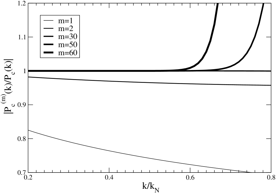
Figure 16: Ratio of the series (55) summed up to the $m$-th term to the exact (numerically evaluated) $P_{c}(k)$. We observe that there is first clear convergence (i.e. approach to unity) as $m$ increases, and then divergence at larger values of $m$.

$P_{th}(k)$ is well approximated by $P_{c}(k)$ if

$$Ak^{n}\gg A^{2}a_{2}k^{2(n+d)-d},$$ (58)

i.e., for

$$Aa_{2}k^{n+d}\ll 1.$$ (59)

It can be checked using Eqs. (56) or (A.1) that $a_{m}/a_{m-1}$ is of order unity for small $m$, so that Eq. (59) corresponds to the criterion Eq. (31) given in the paper. Note that we can rewrite Eq. (59) in terms of the variance of mass in spheres of the theoretical fluctuations, using the approximation (e.g. Gabrielli et al. (2002); Gabrielli et al. (2004a)):

$$\sigma^{2}(R)=bk^{d}P_{th}(k)|_{k=R^{-1}},$$ (60)

where the coefficient $b$ is of order unity. The condition for faithful representation of the PS of the input model at wavenumber $k$ can thus be written:

$$\sigma^{2}(R)|_{k=R^{-1}}\ll 1.$$ (61)

A.2 The case $-d+2<n<\infty$

In this case we must include the UV cut-off in the PS, in order that $d(r)$ be well defined. The latter is then not a simple power-law at all scales as in the precedent case, and we are unable to compute analytically the terms of the series (52). We can, however, compute very simply the first corrections to $P_{th}(k)$. Since $g(0)$ is finite (for $-d+2<n<\infty$), we can rewrite Eq. (52) as

$$P_{c}(k)=e^{-k^{2}g(0)}\int_{\mathbb{R}^{d}}d^{d}re^{-i\mathbf{k}\cdot\mathbf{r}}\left(e^{k^{2}g(r)}-1\right),$$ (62)

where we have used the identity Gabrielli (2004):

$$(2\pi)^{d}\delta(\mathbf{k})=(2\pi)^{d}e^{-k^{2}g(0)}\delta(\mathbf{k})=e^{-k^{2}g(0)}\int d^{d}re^{-i\mathbf{k}\cdot\mathbf{r}}.$$ (63)

Expanding first the exponential containing $g(r)$ in Eq. (62) we obtain

$$P_{c}(k)=e^{-k^{2}g(0)}$$ (64)

$$\times\left(k^{2}\tilde{g}(k)+k^{4}\int_{\mathbb{R}^{d}}d^{d}r[g(r)]^{2}e^{-i\mathbf{k}\cdot\mathbf{r}}+\mathcal{O}(k^{6}[g(r)]^{3})\right).$$

Expansion of the exponential pre-factor then gives

$$P_{c}(k)\simeq P_{th}(k)+$$ (65)

$$k^{4}\left(\int_{\mathbb{R}^{d}}d^{d}r[g(r)]^{2}e^{-i\mathbf{k}\cdot\mathbf{r}}-g(0)\tilde{g}(k)\right).$$

By dimensional analysis one can see that the integral in Eq. (65) scales as $(c_{1}+c_{2}k^{d+2n-4})$, where $c_{1}$ and $c_{2}$ are non-zero constants. For the range of index $n$ considered it follows that:

• For $-d+2<n<2$, the dominant correction to $P_{th}$ comes from the term $\propto g(0)\tilde{g}(k)$ and therefore:

  $$P_{c}(k)\simeq k^{2}\tilde{g}(k)-k^{4}g(0)\tilde{g}(k).$$ (66)

  It follows that the condition for a faithful representation of the theoretical PS ($P_{th}(k)=k^{2}g(k)$) is

  $$g(0)k^{2}\ll 1,$$ (67)

  which corresponds to the condition Eq. (31). For a sharply cut-off theoretical PS

  $$P_{th}(k)=\left\{\begin{array}[]{ll}Ak^{n}&\mbox{for $k\leq k_{c}$};\\ 0&\mbox{otherwise.}\end{array}\right.$$ (68)

  one has

  $$g(0) = \frac{Ak_{c}^{n-1}}{\pi(n-1)}\qquad[d=1]$$ (69)

  $$= \frac{Ak_{c}^{n+1}}{2\pi^{2}(n+1)}\qquad[d=3]$$ (70)

  Dropping the numerical factors, for simplicity, the condition Eq. (67) can be written as

  $$\Delta_{\rm th}^{2}(k)\ll \left(\frac{k}{k_{c}}\right)^{n-1}\qquad[d=1]$$ (72)

  $$\left(\frac{k}{k_{c}}\right)^{n+1}\qquad[d=3]$$

  Since we are considering the case $n>-d+2$ here, this means that Eq. (67) is, for $k<k_{c}$, a more restrictive criterion than that found in the previous case. However, since $\Delta_{\rm th}^{2}(k)$ is a monotonically increasing function of $k$ up to $k_{c}$, the two conditions are essentially equivalent in cosmological NBS, in which one generically imposes a cut-off around $k_{N}$. We note further that the condition is then also equivalent to

  $$\sigma^{2}(R)|_{k_{N}=R^{-1}}\ll 1,$$ (74)

  which is equivalent to (61) (since $\sigma^{2}(R)$ is in this case also a monotonically decreasing function of $R$).

• For $2<n<4$ the main correction comes from the integral in Eq. (65):

  $$P_{c}(k)\simeq k^{2}\tilde{g}(k)+\frac{1}{2}k^{4}\int d^{d}r[g(r)]^{2}e^{-i\mathbf{k}\cdot\mathbf{r}}.$$ (75)

  For the sharply cut-off theoretical PS of Eq. (68), the integral can be evaluated analytically in the limit $\mathbf{k}\to 0$. This gives

  $$P_{c}(k) \simeq Ak^{n}+A^{2}\frac{k^{4}}{2\pi}\frac{k_{c}^{2n-3}}{2n-3}\qquad[d=1]$$ (76)

  $$\simeq Ak^{n}+A^{2}\frac{k^{4}}{2\pi^{2}}\frac{k_{c}^{2n-1}}{2n-1}\qquad[d=3]\,.$$ (77)

  Up to numerical factors of order unity the leading correction is the same as in the previous case, and thus the same criteria apply for the validity of the perturbative expansion as in the previous case.

• For $n>4$ the resulting PS is dominated by the $k^{4}$ correction. The full expression for $P_{c}(k)$ therefore does not approximate $P_{th}(k)$ at sufficiently small $k$.

Appendix B Discreteness corrections to the PS

We analyse further in this appendix the full expansion to all orders of the exact discreteness correction in the PS Eq. (25). Then for the specific case of an input PS with $-d<n<-d+2$, and no UV cut-off, we can evaluate the expression analytically in one dimension. This gives, in particular, an analytic expression for the coefficient of the leading contribution, proportional to $k^{2}$ and allows a precise determination of the range of $k$ in which this term is sub-dominant with respect to the input PS.

Expanding the exponential in Eq. (25) we have

$$\Delta P_{d}(k) \equiv P_{d}(k)-P_{in}(k)$$

$$= \sum_{m=1}^{\infty}(-k^{2})^{m}\int_{\mathbb{R}^{d}}d^{d}re^{-i\mathbf{k}\cdot\mathbf{r}}[d(x)]^{m}\xi_{in}({\bf r})\,.$$

which can be rewritten as

$$\Delta P_{d}(k)=\frac{1}{(2\pi)^{d}}\sum_{m=1}^{\infty}(-k)^{2m}\int_{\mathbb{R}^{d}}d^{d}qD^{(m)}({\mathbf{q}})P_{in}(\mathbf{q}+\mathbf{k})$$ (79)

where

$$D^{(m)}(\mathbf{k}):={\rm FT}[(d(x)^{m}],$$ (80)

where ${\rm FT}$ denotes the FT as defined in Eq. (6). For a pre-initial simple cubic lattice this gives

$$\Delta P_{d}(k)=\sum_{m=1}^{\infty}(-k)^{2m}\sum_{\mathbf{q}\neq 0}D^{(m)}(\mathbf{q}+\mathbf{k})$$ (81)

where

$$\mathbf{q}=k_{N}\mathbf{n},$$ (82)

and $\mathbf{n}$ are triple integers. The smallest $\mathbf{q}$ in the sum (81) is the Nyquist frequency, so that the leading term at small $k$ is the one we discussed in Sect. III.4, proportional to $k^{2}$.

In one dimension all the terms in the series (81) may be calculated analytically, for the case $-d<n<-d+2$ without a UV cut-off. The leading $k^{2}$ term is

$$P_{d}(k)=2Ak_{N}^{n-2}\zeta(2-n)k^{2}+\mathcal{O}(k^{3}).$$ (83)

We can then estimate the scale $k$ up to which this term is sub-dominant compared to the input spectrum:

$$k\raise 1.72218pt\hbox{$<$}\kern-8.00003pt\lower 2.6694pt\hbox{$\sim$}\left(2\zeta(2-n)\right)^{1/n-2}k_{N}.$$ (84)

We note that this scale is independent of the amplitude of the PS (and for $n=-1/2$, $k\raise 1.72218pt\hbox{$<$}\kern-8.00003pt\lower 2.6694pt\hbox{$\sim$}4.2k_{N}$). This result is completely in line with the numerical calculations of the contributions of these terms for various other cases presented in Sect. (III.4).

Appendix C Analytical results in one dimension

In this appendix we give some simplified analytic expressions for the exact PS, mass variance and two point correlation function in one dimension. We have made use of these expressions in our numerical study of various input PS in Sect. V.

We recall first the correlation properties of a simple cubic lattice (in $d$ dimensions for generality) which we will take as the “pre-initial” distribution in what follows. For the reduced two point correlation function one has

$$\tilde{\xi}_{lat}(\mathbf{r}_{1},\mathbf{r}_{2})=\langle\overline{\rho(\mathbf{r})\rho(\mathbf{r}^{\prime})}\rangle-1=\sum_{\mathbf{l}}\delta\left(\mathbf{r}_{1}-\mathbf{r}_{2}-\mathbf{l}\right)-1,$$ (85)

where $\mathbf{l}$ is a generic displacement vector of the lattice. The expression Eq. (33) is simply the Fourier transform of this expression.

Let us now consider the case of one dimension. To compute the variance we use its expression as a function of the PS (see Gabrielli et al. (2002)):

$$\sigma^{2}(R)=\frac{1}{2\pi}\int_{-\infty}^{+\infty}dk\,\left(\frac{\sin(kR)}{kR}\right)^{2}P(k)$$ (86)

or, equivalently, as a function of the correlation function:

$$\sigma^{2}(R)=\frac{1}{8R^{2}}\int_{-\infty}^{+\infty}dx\,\tilde{\xi}(x)\times$$

$$\times \left[-2x\theta(x)+(x-2R)\theta(x-2R)+(x+2R)\theta(x+2R)\right],$$

where $\theta(x)$ is the Heaviside function. Using Eqs. (86) or (C) with (33) or (85) respectively, we obtain the following result for the variance of a lattice with grid spacing equal to unity :

$$\sigma^{2}_{lat}(R)=\sum_{m=-\infty,\neq 0}^{+\infty}\left(\frac{\sin(2\pi mR)}{2\pi mR}\right)^{2}.$$ (88)

As anticipated in the previous section we obtain the same limiting behavior of the variance at large scales as for a homogeneous and isotropic distribution with PS $P(k)\sim k^{n}$ and $n>1$, i.e., $\sigma^{2}(R)\sim 1/R^{d+1}$ with $d=1$.

We now compute an expression for the PS directly from (24), for the case of a one-dimensional system and a “pre-initial” lattice configuration. Using Eq. (85) and rearranging terms we obtain:

$$P(k) = \exp(-k^{2}g(0))\sum_{-\infty,l\neq 0}^{+\infty}\delta(k-2\pi l)$$

$$+ \sum_{l=-\infty}^{+\infty}e^{-ikl}[\exp(-k^{2}d(l)))-\exp(-k^{2}g(0))],$$

where $d(x)\equiv g(0)-g(x)$. The first term on the right hand side of Eq. (C) contains all the divergent terms in the PS. The second term is a regular function of $k$ which has the behavior $P(k)\sim k^{2}g(k)$ at small $k$ if $g(k)\sim k^{\alpha}$ with $\alpha<0$ and $P(k)\sim k^{2}$ if $\alpha>0$, unless $\sum_{l=-\infty}^{+\infty}g(l)=0$, in which case $P(k)\sim k^{2}g(k)$ also for $\alpha>0$.

Performing a Fourier transform of Eq. (24) we obtain the correlation function in the form

$$\tilde{\xi}(x) = \frac{1}{2\pi}\int_{-\infty}^{+\infty}dx^{\prime}\,\sqrt{\frac{\pi}{d(x^{\prime})}}e^{-(x-x^{\prime})^{2}/4d(x^{\prime})}\times$$ (90)

$$\times \left(1+\tilde{\xi}_{in}(x^{\prime})\right)-1.$$

Note that in the limit that no displacements are applied (i.e. $d(x)\to 0$), the argument of the integral is $\delta(x-x^{\prime})$. Thus we recover explicitly for small displacements $\tilde{\xi}(x)\simeq\tilde{\xi}_{in}(x)+\dots$. Substituting Eq. (85) in Eq. (90) we then obtain the result for the specific case of a “pre-initial” lattice configuration:

$$\tilde{\xi}(x)=-1+\sum_{l=-\infty}^{+\infty}\sqrt{\frac{1}{4\pi d(l)}}e^{-(x-l)^{2}/4d(l)}.$$ (91)

To obtain the variance we use the same procedure. Using, for example, Eq. (86) with Eq. (24) we get:

$$\sigma^{2}(R) = -1+\frac{1}{4\sqrt{\pi}R^{2}}\int_{-\infty}^{+\infty}dx\,(1+\tilde{\xi}_{in}(x))\sqrt{\,d(x)}\times$$

$$\times \left[h(x,2R)+h(x,-2R)-2h(x,0)\right]$$

$$+ \frac{1}{8R^{2}}\int_{-\infty}^{+\infty}dx\,(1+\tilde{\xi}_{in}(x))\times$$

$$\times \left[-2f(x,x)+f(x-2R,x)+f(x+2R,x)\right]$$

where

$$f(x,y)=x\,\mathrm{erf}\left(\frac{x}{2\sqrt{d(y)}}\right),\,\,h(x,y)=e^{\frac{-(x+y)^{2}}{4d(x)}}.$$ (93)

Expanding at small $d(x)$ it is possible to obtain also explicitly an expression of the form $\sigma^{2}(R)=\sigma_{lat}^{2}(R)+...$. In the specific case of an initial lattice distribution the variance can be written:

$$\sigma^{2}(R)=-1+\frac{1}{4\sqrt{\pi}R^{2}}\sum_{l=-\infty}^{+\infty}\sqrt{\,d(l)}\times$$

$$\times \left[h(l,2R)+h(l,-2R)-2h(l,0)\right]$$

$$+ \frac{1}{8R^{2}}\sum_{l=-\infty}^{+\infty}\left[-2f(l,l)+f(l-2R,l)+f(l+2R,l)\right].$$

References

- Gabrielli (2004) A. Gabrielli, Phys. Rev. E 70, 066131 (2004), eprint cond-mat/0409594.
- Efstathiou et al. (1985) G. Efstathiou, M. Davis, C. S. Frenk, and S. D. M. White, Astrophys. J. Supp. 57, 241 (1985).
- Couchman (1991) H. M. P. Couchman, Astrophys. J. 368, L32 (1991).
- Bertschinger (1998) E. Bertschinger, Annu. Rev. Astron. Astrophys. 36, 599 (1998).
- Braun and Hepp (1997) W. Braun and K. Hepp, Comm. Math. Phys. pp. 101–113 (1997).
- Spohn (1991) H. Spohn, Large Scale Dynamics of Interacting Particles (Springer-Verlag, 1991).
- Splinter et al. (1998) R. J. Splinter, A. L. Melott, S. F. Shandarin, and Y. Suto, Astrophys. J. 497, 38 (1998).
- Melott et al. (1997) A. L. Melott, S. F. Shandarin, R. J. Splinter, and Y. Suto, Astrophys. J. 479, L79 (1997).
- Hamana et al. (2002) T. Hamana, N. Yoshida, and Y. Suto, Astrophys. J. 568, 455 (2002).
- Diemand et al. (2004a) J. Diemand, B. Moore, J. Stadel, and S. Kazantzidis, Mon. Not. R. Astron. Soc. p. 977 (2004a).
- Diemand et al. (2004b) J. Diemand, B. Moore, and J. Stadel, Mon. Not. R. Astron. Soc. p. 624 (2004b).
- Melott (1990) A. L. Melott, Comments Astrophys. 15, 1 (1990).
- Huterer and Takada (2005) D. Huterer and M. Takada, Astropart. Phys. 23, 369 (2005), eprint astro-ph/0412142.
- Gelb and E. Bertschinger (1994) J. Gelb and E. E. Bertschinger, Astrophys.J 436, 491 (1994).
- Colombi et al. (1994) S. Colombi, F. Bouchet, and R. R. Schaeffer, Astron.Astrophys 281, 301 (1994).
- Colombi et al. (1995) S. Colombi, F. Bouchet, and R. R. Schaeffer, Astron. J. Supp. 96, 401 (1995).
- Colombi et al. (1996) S. Colombi, F. Bouchet, and L. Hernquist, Astrophys.J. Supp. 465, 14 (1996).
- Pen (1997) U. Pen, Astrophys.J. 490, 127 (1997).
- Sirko (2005) E. Sirko, Astrophys.J. 634, 728 (2005).
- Baertschiger and Sylos Labini (2002) T. Baertschiger and F. Sylos Labini, Europhys. Lett. 57, 322 (2002), eprint astro-ph/0109199.
- Dominguez and Knebe (2003) A. Dominguez and A. Knebe, Europhys. Lett. (2003).
- Baertschiger and Sylos Labini (2003) T. Baertschiger and F. Sylos Labini, Europhys. Lett. 63, 633 (2003), eprint astro-ph/0309387.
- Knebe and Dominguez (2003) A. Knebe and A. Dominguez, Publ. Astron. Soc. Pac. 20 (2003).
- Joyce and Marcos (2006) M. Joyce and B. Marcos, Quantification of discreteness effects in cosmological n-body simulations: 2. evolution up to shell crossing (2006), in preparation.
- Melott and Shandarin (1990) A. L. Melott and S. F. Shandarin, Astrophys. J. 364, 396 (1990).
- Bagla and Padmanabhan (1997) J. S. Bagla and T. Padmanabhan, Mon. Not. R. Astron. Soc. 286, 1023 (1997), eprint astro-ph/9605202.
- Costin and Lebowitz (2004) O. Costin and J. Lebowitz, J. Phys. Chem. B., 19614 (2004).
- Crawford et al. (2003) J. R. Crawford, S. Torquato, and F. H. Stillinger, J. Chem. Phys. p. 7065 (2003).
- Uche et al. (2006) O. Uche, S. Torquato, and F. H. Stillinger, Physica A, 21 (2006).
- Zeldovich (1970) Y. B. Zeldovich, Astron. & Astrop. pp. 84–89 (1970).
- Buchert (1992) T. Buchert, Mon. Not. R. Astr. Soc. 254, 729 (1992).
- White (1993) S. White, Lectures given at les houches (1993), eprint astro-ph/9410043.
- Scoccimarro (1998) R. Scoccimarro, Mon. Not. R. Astron. Soc. 299, 1097 (1998).
- Valageas (2002) P. Valageas, Astron. Astrophys 385, 761 (2002).
- Schneider and Bartelmann.M. (1995) P. Schneider and Bartelmann.M., Mon. Not. R. Astron. Soc. 273, 475 (1995).
- Taylor and Hamilton (1996) A. Taylor and A. Hamilton, Mon. Not. R. Astron. Soc. 282, 767 (1996).
- Gabrielli et al. (2004a) A. Gabrielli, F. Sylos Labini, M. Joyce, and L. Pietronero, Statistical Physics for Cosmic Structures (Springer, 2004a).
- Gabrielli et al. (2002) A. Gabrielli, M. Joyce, and F. Sylos Labini, Phys. Rev. D 65, 083523 (2002).
- (39) E. Bertschinger, Cosmics: Cosmological initial conditions and microwave anisotropy codes, eprint astro-ph/9506070.
- Baus and Hansen (1980) M. Baus and J.-P. Hansen, Physics Reports 59, 1 (1980).
- Smith et al. (2003) R. E. Smith, J. A. Peacock, A. Jenkins, S. D. M. White, C. S. Frenk, F. R. Pearce, P. A. Thomas, G. Efstathiou, and H. M. P. Couchman, Mon. Not. R. Astron. Soc. 341, 1311 (2003).
- Zeldovich (1965) Y. B. Zeldovich, Adv. Astron. 3, 241 (1965).
- Zeldovich and Novikov (1983) Y. Zeldovich and I. Novikov, Relativistic Astrophysics (Univ. Chicago Press, Chicago, 1983).
- Peebles (1993) P. J. E. Peebles, Principles of physical cosmology (Princeton Series in Physics, Princeton, NJ: Princeton University Press, —c1993, 1993).
- Gabrielli et al. (2004b) A. Gabrielli, M. Joyce, B. Marcos, and P. Viot, Europhys. Lett. 66, 1 (2004b), eprint astro-ph/0303169.
- Jenkins et al. (1998) A. Jenkins, C. S. Frenk, F. R. Pearce, P. A. Thomas, J. M. Colberg, S. D. M. White, H. M. P. Couchman, J. A. Peacock, G. Efstathiou, and A. H. Nelson, Astrophy. J. 499, 20 (1998).
- Little et al. (1991) B. Little, D. Weinberg, and C. Park, Mon. Not. R. Astr. Soc. 253, 295 (1991).
- Yamaguchi et al. (2004) Y. Y. Yamaguchi, J. Barré, F. Bouchet, T. Dauxois, and S. Ruffo, Physica A 337, 36 (2004), eprint cond-mat/0312480.