Two viable quintessence models of the Universe: confrontation of theoretical predictions with observational data

We use some of the recently released observational data to test the viability of two classes of minimally coupled scalar field models of quintessence with exponential potentials for which exact solutions of the Einstein equations are known. These models are very sturdy, depending on only one parameter - the Hubble constant. To compare predictions of our models with observations we concentrate on the following data: the power spectrum of the CMBR anisotropy as measured by WMAP, the publicly available data on type Ia supernovae, and the parameters of large scale structure determined by the 2-degree Field Galaxy Redshift Survey (2dFGRS). We use the WMAP data on the age of the universe and the Hubble constant to fix the free parameters in our models. We then show that the predictions of our models are consistent with the observed positions and relative heights of the first 3 peaks in the CMB power spectrum, with the energy density of dark energy as deduced from observations of distant type Ia supernovae, and  bf with parameters of the large scale structure as determined by 2dFGRS, in particular with the average density of dark matter. Our models are also consistent with the results of the Sloan Digital Sky Survey (SDSS). Moreover, we investigate the evolution of matter density perturbations in our quintessential models, solve exactly the evolution equation for the density perturbations, and obtain an analytical expression for the growth index $f$. We verify that the approximate relation $f\simeq\Omega_{{\rm M}}^{\alpha}$ also holds in our models.

1 Introduction

Recent observations of the type Ia supernovae and CMB anisotropy strongly indicate that the total matter-energy density of the universe is now dominated by some kind of dark energy or the cosmological constant $\Lambda$ (Riess & al. (1998); Riess (2000); Perlmutter & al. (1999); Riess & al. 2004 ). The origin and nature of this dark energy remains unknown (Zeldovich (1967); Weinberg (1989); Carroll (2001)).
In the last several years a new class of cosmological models has been proposed. In these models the standard cosmological constant $\Lambda$-term is replaced by a dynamical, time-dependent component - quintessence or dark energy - that is added to baryons, cold dark matter (CDM), photons and neutrinos. The equation of state of the dark energy is given by $w_{Q}\equiv\rho_{Q}/p_{Q}$, $\rho_{Q}$ and $p_{Q}$ being, respectively, the pressure and energy density, and $-1\leq w_{Q}<0$, which implies a negative contribution to the total pressure of the cosmic fluid. When $w_{Q}=-1$, we recover a constant $\Lambda$-term. One of the possible physical realizations of quintessence is a cosmic scalar field, minimally coupled to the usual matter action (Peebles & Ratra (1988); Caldwell & al. (1998)). Such a field induces dynamically a repulsive gravitational force, causing an accelerated expansion of the Universe, as recently discovered by observations of distant type Ia supernovae (SNIa) (Perlmutter & al. (1999); Riess & al. (1998); Riess & al. 2004 ) and confirmed by WMAP observations (Spergel & al. (2003)). Accelerated expansion together with the strong observational evidence that the Universe is spatially flat ( de Bernardis & al. (2000); Spergel & al. (2003)) calls for an additional component and quintessence could be responsible for the missing energy in a flat Universe with a subcritical matter density. Quintessence drives the cosmological expansion at late times and also influences the growth of structure arising from gravitational instability. Dark energy could cluster gravitationally only on very large scales ($\geq 100$ Mpc), leaving an imprint on the microwave background anisotropy (Caldwell & al. (1998)); on small scales, fluctuations in the dark energy are damped and they do not influence the evolution of perturbations in the pressureless matter ( Ma & al. (1999)). On the scales we are considering in the following, we assume that quintessence behaves as a smooth component, so that in our analysis the formation of clusters is due only to matter condensation, while the quintessence alters only the background cosmic evolution. The leading candidates for the dark energy as suggested by fundamental physics include vacuum energy, a rolling scalar field, and a network of slight topological defects (Turner (2000); Cline (2001)). Moreover, an eternally accelerating universe seems to be at odds with some formulations of the string theory (Fischler & al. (2003)). However, this is still controversial. Actually in the last few years it has been suggested that string theory could be compatible with the presently considered cosmological models (see for example,  Hellerman, Kalper & Susskind (2001); Townsend & Wohlfarth (2003); Gibbons & Hull (2001) and references therein). This has stimulated a revival of interest in the exponential scalar field quintessence. In different scenarios, such exponential potentials can reproduce the present accelerated expansion of the universe and some predict future deceleration. Moreover, despite the criticism that exponential potentials require fine tuning, recently several authors have pointed out that the degree of fine tuning needed in this case is not greater than in other scenarios (Cline (2001); Rubano & Scudellaro (2001); Cardenas & al. (2002)).
In this work we show that the two models of quintessence for which general exact solutions of the Einstein equation are known are compatible with recent observational data, in particular with the power spectrum of the temperature anisotropy of the CMBR, the observations of type Ia supernovae, and the parameters of the large scale structure of matter distribution. As a first step we introduce a new parametrization of quintessence models considered by Rubano et al. and Rubano & Scudellaro  (Rubano & al. (2002); Rubano & Scudellaro (2001)), which avoids the problem of branching of solutions highlighted in Cardenas & al., (2002).
Since the physical features of these models will be extensively discussed in a forthcoming paper, in Sect. 2, we simply present the basic equations of the quintessence models used in this paper. In Sect. 3 the linear perturbation equation is solved for the two potentials and the growth of density perturbations is discussed; in Sect. 4 we show that predictions of our models are compatible with the observationally established power spectrum of CMB anisotropy, the SNIa data, and the results of estimates of the average mass density of the universe from galaxy redshift surveys. In Sect. 5 we discuss the possibility of constraining the equation of state of dark energy by age estimates of the universe. Sect. 6 is devoted to final conclusions.

2 Model description

In this paper we consider two quintessence models, with a single and a double exponential potential, for which exact analytic solutions are available. The discussion of the physical properties as well as the mathematical features of these models goes beyond the aims of this work; they are presented in   Rubano & al. (2004). Here we will only give the basic relations.

2.1 The single exponential potential

We investigate spatially flat, homogeneous, and isotropic cosmological models filled with two non-interacting components: pressureless matter (dust) and a scalar field $\varphi$, minimally coupled with gravity. We first consider the potential introduced in  Rubano & Scudellaro (2001),

$$V(\varphi)\propto\exp\left\{-\sqrt{3\over 2}\varphi\right\}.$$ (1)

For this potential the following substitution

$$a = {\left(u\,v\right)}^{\frac{1}{3}}\,,$$ (2)

$$\varphi = -\left({\sqrt{\frac{2}{3}}}\,\log(\frac{u}{v})\right),$$ (3)

where $a$ is the scale factor, makes it possible to integrate the Friedman equations exactly. Setting as usual $a(0)=0$ we have

$$u = u_{1}t,$$ (4)

$$v = v_{1}t+v_{2}t^{3},$$

where $u_{1}$, $v_{1}$ and $v_{2}$ are integration constants, so for $a(t)$, we get

$$a^{3}(t)=u_{1}v_{2}t^{2}(t^{2}+{v_{1}\over v_{2}})\,.$$ (5)

If by $H$ we denote the time dependent Hubble parameter then

$$H={4\over{3t}}\left({{t^{2}+{v_{1}\over{2v_{2}}}\over{t^{2}+{v_{1}\over v_{2}}}}}\right).$$ (6)

To determine the integration constants $u_{1}$, $v_{1}$ and $v_{2}$ we set the present time $t_{0}=1$. This fixes the time-scale according to the (unknown) age of the universe. That is to say that we are using the age of the universe, $t_{0}$, as a unit of time. We then set $a_{0}=a(1)=1$, which is standard, and finally $H_{0}=H(1)$. Because of our choice of time unit it turns out that our $H_{0}$ is not the same as the $H_{0}$ that appears in the standard FRW model. The two conditions specified above allow one to express all the basic cosmological parameters in terms of $H_{0}$. With these choices the whole history of the universe has been squeezed into the range of time $[0,1]$. Moreover this model is uniquely parametrized by $H_{0}$ only. Explicitly we have:

$$a^{3}(t) = {t^{2}\over 2}[(3H_{0}-2)t^{2}+4-3H_{0}],$$ (7)

$$H(t) = {{2\left(2(3H_{0}-2)t^{2}+4-3H_{0}\right)}\over{3t\left((3H_{0}-2)t^{2}+4-3H_{0}\right)}},$$ (8)

$$\Omega_{M} = {{(4-3H_{0})\left((3H_{0}-2)t^{2}+4-3H_{0}\right)}\over[2(3H_{0}-2)t^{2}+4-3H_{0}]^{2}},$$ (9)

$$\Omega_{\varphi} = {{(3H_{0}-2)t^{2}\left(4(3H_{0}-2)t^{2}+3(4-3H_{0})\right)}\over[2(3H_{0}-2)t^{2}+4-3H_{0}]^{2}}.$$ (10)

Therefore now the omega parameters of matter and the dark energy are

$$\Omega_{M_{0}}\equiv\Omega_{M}(t=1)=\frac{2(4-3\,H_{0})}{9\,H_{0}^{2}}\,,$$ (11)

$$\Omega_{\varphi_{0}}\equiv\Omega_{\varphi}(t=1)=\frac{\left(3\,H_{0}-2\right)\,\left(3\,H_{0}+4\right)}{9\,H_{0}^{2}}\,.$$ (12)

The equation of state of dark energy evolves with time and the parameter $w$ is given by

$$w=-\frac{1}{2}+\frac{3(3\,H_{0}-4)}{6(4-3\,H_{0})+8\left(3\,H_{0}-2\right)t^{2}}\,,$$ (13)

so that today we have

Figure 1: Time dependence of the scale factor $a$ for the single exponential potential, for $H_{0}=0.97$.

Figure 2: Redshift dependence of the parameter $w$ for the single exponential potential, for $H_{0}=0.97$.

$$w_{0} = -{8-3H_{0}\over 4+3H_{0}}\,.$$ (14)

In Fig. 1 we show the time evolution of the scale factor while the redshift dependence of $w$ is plotted in Fig. 2. Asymptotically for $t\rightarrow\infty$, $a(t)\sim t^{4/3}$ and therefore in this model the universe is eternally accelerating and possesses a particle horizon. The relation between the dimensionless time $t$ and the redshift $z$ is given by

$$z={2^{1\over 3}\over\left[t^{2}((3H_{0}-2)t^{2}+4-3H_{0})\right]^{1\over 3}}-1.$$ (15)

We shall compare the predictions of the above model with a flat cosmological model filled in with matter and the cosmological constant. In this case, the redshift dependent Hubble parameter is

$$H(z)={\bar{H}}_{0}\sqrt{{\Omega_{{\rm M0}}}(1+z)^{3}+(1-{\Omega_{{\rm M0}}})}\,,$$ (16)

where ${\bar{H}}_{0}$ is the standard Hubble constant. This class of models has two free parameters, ${\Omega_{{\rm M0}}}$ and ${\bar{H}}_{0}$, where

$${\bar{H}}_{0}={100\,h\,\,{\rm km}\,{\rm s}^{-1}\,{\rm Mpc}^{-1}}.$$

Let us assume that the age of the universe is

$$t_{0}=\gamma{\times}1{\rm Gy}=\,3.15\,10^{16}\,\gamma\,{\rm s},$$

where $\gamma$ is a constant to be determined by astronomical observations. With this definition it is possible to relate the value of $H_{0}$ to the small $h={\bar{H}}_{0}/100$ of the standard FRW model. It turns out that

$$H_{0}=0.1\,h\,\,\gamma.$$ (17)

If we accept that $t_{0}=\,13.7\,$ Gy as given by the WMAP team (Spergel & al. (2003)) then $H_{0}=1.37h$.

2.2 The double exponential potential

As the second example we consider the following double exponential potential:

$$V(\varphi) = \left(A\exp{({1\over 2}\sqrt{{3\over 2}\varphi})}-B\exp{(-{1\over 2}\sqrt{{3\over 2}}\varphi)}\right)^{2}$$

$$\equiv A^{2}\exp{\left(\sqrt{{3\over 2}\varphi}\right)}+B^{2}\exp{\left(-\sqrt{{3\over 2}}\varphi\right)}-2AB,$$

where $A$ and $B$ are constants. As we see, if we take $A,B>0$ this model contains in a certain sense an intrinsic negative cosmological constant, but this does not lead to the re-collapsing typical in such cases. It turns out that this is an eternally expanding model, with alternate periods of accelerating and decelerating expansion. In the following we denote $\omega^{2}=3AB$.
For this model exact solutions of the Einstein equations with scalar field exist, but their explicit mathematical form is rather complicated. General properties of these solutions are discussed in   Rubano & al. (2004). Here we observe that if we use the same parametrization as in the previous case, e.g. taking the age of the Universe as a unit of time, the solution will depend on only two parameters: $H_{0}$ and $\omega$. In order to get physically acceptable values of $\Omega_{\varphi}$ (i.e $\Omega_{\varphi}>0$) we have to take $\omega\leq 2$. However, in our analysis we use a more restrictive range, $0\leq\omega\leq 1$, as we will discuss in the next sections. We will see however that in this range of values of $\omega$ the matter density parameter ${\Omega_{{\rm M0}}}$ is changing only slightly. In this case we obtain the following expressions for $a$, $H$ and $\Omega_{\varphi}$, which are the main quantities we need:

$$a^{3}(t)={{(3H_{0}\sin^{2}{\omega}-\omega\sin{2\omega})t^{2}-(3H_{0}-2)\sin^{2}{\omega t}}\over{2\sin^{2}{\omega}-\omega\sin{2\omega}}},$$ (19)

$$H={2\over 3}\left({t-\displaystyle{{\left(3H_{0}-2\right)\omega\sin{2\omega t}}\over{2(3H_{0}\sin{\omega}-\omega\sin{2\omega})}}\over t^{2}-\displaystyle{{(3H_{0}-2)\sin^{2}{\omega t}}\over{(3H_{0}-2)\sin{\omega}-\omega\sin{2\omega}}}}\right),$$ (20)

$$\Omega_{\varphi}=\left[(\omega t\cos{\omega t}-\sin{\omega t})^{2}+\omega^{2}\sin^{2}{\omega t}(t^{2}-{{(3H_{0}-2)\sin^{2}{\omega t}}\over{(3H_{0}\sin^{2}{\omega}-\omega\sin{2\omega})}})\right]{\times}$$

$${\left(3H_{0}-2\right)\over(3H_{0}\sin^{2}{\omega}-\omega\sin{2\omega})\left[t-{{(3H_{0}-2)\omega}\sin{2\omega t}\over{2(3H_{0}\sin{\omega}-2\omega\cos{\omega})}}\right]^{2}}\,,$$ (21)

where $H_{0}$ and $\omega$ are constants. Since we consider a flat model, $\Omega_{M}=1-\Omega_{\varphi}$. Note that when $t\rightarrow\infty$, $\Omega_{\phi}\rightarrow{\rm const}$ and in the generic case this constant is smaller than 1 and therefore, when $t\rightarrow\infty$, $\Omega_{M}$ does not vanish, so at the late stages of evolution of this model dark energy and matter coexist. For large $t$, $a(t)\sim t^{2/3}$ though $\Omega_{\varphi}\not=0$ and evolution of this model resembles the matter-dominated phase of the standard FRW universe, hence in this case the particle horizon does not appear. At the present epoch we get

$$\Omega_{\varphi_{0}}\equiv\Omega_{\varphi}(t=1)=$$ (22)

$$\frac{\left(3\,H_{0}-2\right)\,\left[3H_{0}\left(\omega\sin{2\omega}-2\sin^{2}{\omega}\right)+2\,\omega\,(\sin{2\omega}-2\,\omega)\right]}{9\,{H_{0}}^{2}\,\left(\omega\,\sin{2\,\omega}-2\sin^{2}{\omega}\right)}\,,$$

$$\Omega_{M_{0}}\equiv\Omega_{M}(t=1)={\left(2\over 3H_{0}\right)}^{2}\frac{\omega\,\sin{2\,\omega}+3\,H_{0}\cos^{2}{\omega}-2\,{\omega}^{2}\,}{\left(\omega\,\sin{2\omega}-2\,\sin^{2}{\omega}\right)}\,.$$ (23)

When $\omega$ is small we obtain the following simple approximated formula for $\Omega_{\varphi_{0}}$ and $\Omega_{M0}$

$$\Omega_{\varphi_{0}} \cong \frac{\left(3\,H_{0}-2\right)\,\left(30\,\left(3\,H_{0}+4\right)-\left(9\,H_{0}+4\right)\,{\omega}^{2}\right)}{27\,{H_{0}}^{2}\,\left(10-{\omega}^{2}\right)}\,,$$ (24)

$$\Omega_{M_{0}} \cong \frac{2\,\left(4\,\left(30-\omega^{2}\right)-3\,H_{0}\,\left(30+\omega^{2}\right)\right)}{27\,H_{0}^{2}\,\left(10-\omega^{2}\right)}.$$ (25)

Figure 3: Time dependence of the scale factor $a$ for the double exponential potential, for $H_{0}=0.97$, and $\omega=0.1$.

For $\omega$ in the range $(0,1)$, Eq. (24) shows that the dependence of $\Omega_{\varphi_{0}}$ on $\omega$ can be neglected. Actually, in analyzing the observational data we will set $\omega=0.1$ . In the double exponential potential model the relation between the dimensionless time $t$ and the redshift $z$ is given by

Figure 4: Redshift dependence of the parameter $w$, for the double exponential potential, with $H_{0}=0.97$ and $\omega=0.1$.

$$1+z = \frac{{\left(\omega\,\sin{2\omega}-2\sin^{2}\omega\right)}^{1\over 3}}{\left[t^{2}\left(\omega\sin{2\omega}-3H_{0}\sin^{2}{\omega}\right)+\left(3H_{0}-2\right)\sin^{2}{\omega\,t}\right]^{\frac{1}{3}}}\,,$$ (26)

which for small values of $\omega$ and $t$ can be simplified to

$$1+z \simeq {{2^{1\over 3}t^{-{2\over 3}}}\over\left[4-3H_{0}-{2\over 15}\left(3\,H_{0}-2\right)\omega^{2}\right]^{1\over 3}}\,.$$ (27)

Fig. 3 shows the time evolution of the scale factor $a$. As shown in Fig. 4 the equation of state for this double exponential potential evolves with time. The relation between $H_{0}$ and the value of the Hubble constant in the FRW model is the same as in the single exponential case.

3 Growth of density perturbations

The equation describing evolution of the CDM density contrast, $\delta_{M}\equiv\delta\rho_{M}/\rho_{M}$, for perturbations inside the horizon, is (Peebles (1980); Ma & al. (1999))

$$\ddot{\delta}_{M}+2H(t)\dot{\delta}_{M}-4\pi{\rm G}\rho_{M}\delta_{M}=0,$$ (28)

where the dot denotes the derivative with respect to time. In Eq. (28) the dark energy enters through its influence on the expansion rate $H(t)$. We shall consider Eq. (28) only in the matter dominated era, when the contribution of radiation is really negligible.

3.1 The single exponential case

For the model with the single exponential potential described by the Eq. (1), the differential equation (28) reduces to

$$\frac{d^{2}\delta_{M}}{dt^{2}}+\frac{4}{3t}\,\frac{\,\left[4-3H_{0}-2(2-3\,H_{0})\,t^{2}\right]}{(4\,-3\,H_{0}-(2\ -3\,H_{0})\,t^{2})}\frac{d\delta_{M}}{dt}-\frac{2(4-3\,{H_{0}})\delta_{M}}{3t^{2}\left[4-3H_{0}\,-(2-3\,H_{0})t^{2}\right]}=0.$$ (29)

Equation (29) is of Fuchsian type with 3 finite regular singular points, and a regular point at $t\rightarrow\infty$; i.e. it is an hypergeometric equation, which has two linearly independent solutions, the growing mode $\delta_{+}$ and the decreasing mode $\delta_{-}$. Solutions of this equation can be expressed in terms of the hypergeometric function of the second type $\ {}_{2}F_{1}$. We get

$$\delta_{-}\propto\frac{1}{t}\ _{2}F_{1}\left[-\frac{1}{2},\frac{1}{3},\frac{1}{6};\left({{3H_{0}-2}\over{3H_{0}-4}}\right)\,t^{2}\right],$$ (30)

and

$$\delta_{+}\propto t^{\frac{2}{3}}\,\ _{2}F_{1}\left[\frac{1}{3},\frac{7}{6},\frac{11}{6},\left({{3H_{0}-2}\over{3H_{0}-4}}\right)\,t^{2}\right].$$ (31)

In the linear perturbation theory the peculiar velocity field ${\bf v}$ is determined by the density contrast (Peebles (1980); Padmanabhan (1993))

$${\bf v}({\bf x})=H_{0}\frac{f}{4\pi}\int\delta_{M}({\bf y})\frac{{\bf x}-{\bf y}}{\left|{\bf x}-{\bf y}\right|^{3}}d^{3}{\bf y},$$ (32)

where the growth index $f$ is defined as

$$f\equiv\frac{d\ln\delta_{M}}{d\ln a}\,,$$ (33)

$a$ is the scale factor. According to our conventions, using only the growing mode, we get

Figure 5: $\ln f$ versus $\ln{\Omega_{\rm M}}$ in the single exponential potential model.

$$f = \frac{4-3\,H_{0}+\left(3\,H_{0}-2\right)\,t^{2}}{4-3\,H_{0}+2\,\left(3\,H_{0}-2\right)\,t^{2}}\left\{\ {}_{2}F_{1}\left[\frac{1}{3},\frac{7}{6},\frac{11}{6},\left({{3H_{0}-2}\over{3H_{0}-4}}\right)\,t^{2}\right]+\right.$$

$$\left.\frac{7\,\left(3\,H_{0}-2\right)\,t^{2}}{11\,\left(3\,H_{0}-4\right)}\ _{2}F_{1}\left[\frac{4}{3},\frac{13}{6},\frac{17}{6},\left({{3H_{0}-2}\over{3H_{0}-4}}\right)\,t^{2}\right]\right\}\left({\ {}_{2}F_{1}\left[\frac{1}{3},\frac{7}{6},\frac{11}{6},\left({{3H_{0}-2}\over{3H_{0}-4}}\right)\,t^{2}\right]}\right)^{-1}\,.$$

The growth index is usually approximated by $f\simeq{\Omega_{\rm M}}^{\alpha}$. For $\Lambda$CDM models, $\alpha\simeq 0.55$ (see Silveira & Waga (1994); Wang & Steinhardt (1998); Lokas et al. (2004)). In Fig. 5, we show the logarithm of $f$ as a function of the logarithm of ${\Omega_{\rm M}}$ for the single exponential potential. It turns out that $\alpha\simeq 0.57$ provides a good approximation to the model. In Fig. 6 we see that $\alpha$ can be considered a constant during the late stages of the universe evolution.

Figure 6: Redshift dependence of the exponent $\alpha$ in the single exponential potential model. We see that $\alpha$ can be considered constant during the cosmic expansion.

3.2 The double exponential case

For the model with double exponential potential described by Eq. (2.2), the differential equation (28) becomes more complicated, it assumes the form

$$\frac{d^{2}\delta_{M}}{dt^{2}}+\frac{2}{3}\,\,\left[{2t\left(3H_{0}\sin^{2}\omega-\omega\sin{2\omega}\right)+\omega\,\sin(2\omega t)\left(2-3\,{H_{0}}\right)\over t^{2}\left(3H_{0}\sin^{2}\omega-\omega\sin{2\,\omega}\right)+\sin^{2}(\omega t)\left(2-3{H_{0}}\right)}\right]\frac{d\delta_{M}}{dt}$$ (35)

$$-{4\left[3H_{0}\left(\omega^{2}-\sin^{2}{\omega}\right)+\omega\left(\sin{2\omega}-2\omega\right)\right]\over 3\left[2\left(3H_{0}-2\right)\sin^{2}{\omega t}+2t^{2}\left(\omega\sin{2\omega}-3H_{0}\sin^{2}{\omega}\right)\right]}\delta_{M}=0\,.$$

Eq. (35) does not admit exact analytic solutions. However, since with our choice of normalization the whole history of the Universe is confined to the range $t\in[0,1]$, and since we choose $\omega\leq 1$, we can expand the trigonometric functions appearing in Eq. (35) in series around $t=1$, obtaining an integrable differential equation, which is again a hypergeometric equation. For the growing mode we get

$$\delta_{+}\propto t^{2\over 3}\ _{2}F_{1}\left[-\frac{1}{3},\frac{7}{6},\frac{11}{6};{\left(2-3H_{0}\right)\,t^{2}\over{2\left[3H_{0}-4-{2\over 5}(H_{0}-2)\omega^{2}\right]}}\right]\,.$$ (36)

We use the growing mode $\delta_{+}$ to construct the growth index $f$; according to Eq. (33) we obtain

$$f={A_{1}\over A_{2}},$$ (37)

where

$$A_{1}={105\over 4}(3H_{0}-4)^{3}(2-3H_{0})t^{2}\ _{2}F_{1}\left[-\frac{4}{3},\frac{16}{6},\frac{17}{6};{\left({2-3H_{0}}\right)\,t^{2}\over{2\left[3H_{0}-4-{2\over 5}(H_{0}-2)\omega^{2}\right]}}\right]$$ (38)

$${\times}\left(33\left[3H_{0}-4-{2\over 5}(H_{0}-2)\omega^{2}\right]\ _{2}F_{1}\left[-\frac{1}{3},\frac{7}{6},\frac{11}{6};{\left(2-3H_{0}\right)\,t^{2}\over{2\left[3H_{0}-4-{2\over 5}(H_{0}-2)\omega^{2}\right]}}\right]\right)\,,$$

$$A_{2}=t^{2}\omega^{2}(3H_{0}-2)\left[\omega^{2}\left(176+39(H_{0}-4)H_{0}\right)+(H_{0}-2)(3H_{0}-4)\right]$$ (39)

$$+{5\over 2}(4-3H_{0})\left[(3H_{0}-2)t^{2}+4-3H_{0}\right]\,.$$

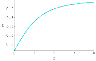
Figure 7: Behaviour of the exact and approximate growth index $f$ for the double exponential potential model. The solid line is the exact function and the dashed one the approximate function.

In Fig. 7 we see how accurate our approximate $f$ is, in comparison with that obtained by numerical integration of Eq. (35). In this case the growth index is approximated by $f\simeq{\Omega_{\rm M}}^{\alpha}$, where $\alpha\simeq 0.57$.

4 Observational data and predictions of our models

The scalar field models of quintessence described in the previous sections depend on at most two arbitrary parameters that admit a simple physical interpretation. The cosmological model with single exponential potential of Eq. (1) is uniquely parametrized by the Hubble constant $H_{0}$ only, while the model with double exponential potential of Eq. (2.2) is parametrized by $H_{0}$ and the frequency $\omega$. We have shown, however, that the actual value of $\omega$ affects only slightly the most important quantities as, for instance, the density parameter $\Omega_{\varphi_{0}}$ (see Eq. (24)). Comparing predictions of this model with observations we will assume that $\omega=0.1$. Using the WMAP data on the age of the universe $t_{0}=13.7\pm 0.2$ Gy and on the Hubble constant ${\bar{H}_{0}}=71\pm 5$ kms^-1Mpc^-1 (Spergel & al. (2003)), from Eq.(17) we get that our $H_{0}=0.97\pm 0.08$. Once $H_{0}$ and $\omega$ are fixed our models are fully specified and do not contain any free parameters. In particular in the single exponential potential model we have $\Omega_{\varphi_{0}}=0.73\pm 0.09$ and $w_{0}=-0.73\pm 0.06$ and in the double exponential potential model $\Omega_{\varphi_{0}}=0.74\pm 0.10$ and $w_{0}=-0.73\pm 0.07$. We can now compare predictions of our models with available observational data to test their viability. In Fig. 8 that with these values of $H_{0}$ and $h$, the transition redshift from a decelerating to an accelerating phase in the evolution of the universe falls very close to $z=0.5$, in agreement with recent results coming from the SNIa observations (Riess & al. 2004 ).

Figure 8: Behaviour of the second derivative of the scale factor in the single exponential potential with $H_{0}=0.97$, $\Omega_{\varphi_{0}}=0.75$. Please note that the transition from a decelerating to an accelerating expansion occurs close to $z=0.5$, as predicted by recent observations of SNIa $z_{t}=0.46\pm 0.13$ (Riess & al. 2004 ).

In the following we concentrate on three different kinds of observations: namely the measurements of the anisotropy of the CMBR by the WMAP team (Bennett & al (2003); Spergel & al. (2003)), on the high z supernovae of type Ia, and the observations of the large scale structure by the 2dFGRS Team (Hawkins & al. (2003)).

4.1 Constraints from CMBR anisotropy observations

After the discovery of the cosmic microwave background radiation by Penzias & Wilson (1965) several experiments have been devoted to measuring the temperature fluctuations of CMBR. The recently released Wilkinson Microwave Anisotropy Probe (WMAP) data opened a new epoch in CMBR investigations, allowing strict tests of realistic cosmological models. The WMAP data are powerful for cosmological investigations since the mission was carefully designed to limit systematic errors, which are actually very low (Bennett & al (2003)). The WMAP measured the power spectrum of the CMBR temperature anisotropy, precisely determining positions and heights of the first two peaks. It turns out that the separation of the peaks depends on the amount of dark energy today, the amount at the last scattering, and some averaged equation of state. Assuming that the radiation propagates from the last scattering surface up to now in such a way that the positions of the peaks are not changed, the peaks appear at multipole moments

$$l_{n} = {\eta_{0}-\eta_{rec}\over c_{s}\eta_{rec}}n\pi\equiv nl_{A},$$ (40)

where $\eta$ is the conformal time ( then $\eta_{rec}$ and $\eta_{0}$ are respectively its value at the recombination and today), the speed of sound $c_{s}$ is assumed approximately constant during recombination, and $l_{A}$ is the acoustic horizon scale. In models with quintessence Eq. (40) should be modified and rewritten as (Doran & Lilley (2002); Doran & al. (2002); Hu & Dodelson (2002); Hu & al. (2001))

$$l_{n} = l_{A}(n-\zeta_{n}),$$ (41)

where $\zeta_{n}=\zeta+\Delta\zeta$, here $\Delta\zeta$ is a general phase shift, whose form for the first three peaks is given in (Doran & Lilley (2002)), and $\zeta=a_{1}(r_{rec})^{a_{2}}+\Omega_{\phi}^{rec}$, where

$$r_{rec}={\rho_{r}(z_{rec})\over\rho_{M}(z_{rec})},$$ (42)

$$\Omega_{\varphi}^{rec}=\eta_{rec}^{-1}\int^{\eta_{rec}}_{0}\Omega_{\phi}(\eta)d\eta.$$ (43)

The constants $a_{1}$ and $a_{2}$ are fit parameters also furnished in Doran & Lilley (2002), Doran & al. (2002), and $\rho_{r}$ is the radiation density. It is possible to obtain an analytic formula for $l_{A}$. Following Doran & Lilley and introducing

$$\langle w_{0}\rangle={\int^{\eta_{rec}}_{0}\Omega_{\varphi}(\eta)w(\eta)d\eta\over\int^{\eta_{rec}}_{0}\Omega_{\varphi}(\eta)d\eta},$$ (44)

we get

$$l_{A} = \pi c^{-1}_{s}\left[{F(\Omega_{\varphi_{0}},\langle w_{0}\rangle)\over\sqrt{a_{rec}(1-\Omega_{\varphi}^{rec})}}\left\{1+\left({\Omega_{r_{0}}\over a_{rec}(1-\Omega_{\varphi_{0}})}\right)^{1\over 2}+{\Omega_{r_{0}}\over 2a_{rec}(1-\Omega_{\varphi_{0}})}\right\}-1\right]\,,$$ (45)

where

$$F(\Omega_{\varphi_{0}},\langle w_{0}\rangle)={1\over 2}\int^{1}_{0}dx\left(x+{\Omega_{\varphi_{0}}\over{1-\Omega_{\varphi_{0}}}}x^{1-3\langle w_{0}\rangle}+{\Omega_{r_{0}}(1-x)\over{1-\Omega_{\varphi_{0}}}}\right)^{-{1\over 2}}\,,$$ (46)

and $a_{rec}$ is the value of the scale factor at recombination. Using Eqs. (44), (45) and (41) in our single exponential potential model, we find that $\langle w_{0}\rangle=-0.85$, and we get the following values of $l$ specifying the positions of the peaks

$$l_{1} = 225^{+11}_{-12}\,,$$ (47)

$$l_{2} = 546^{+27}_{-24}\,,$$ (48)

$$l_{3} = 830^{+42}_{-29}\,.$$ (49)

These values are consistent with the observed positions of the peaks as measured by Boomerang (de Bernardis & al. (2000)) and WMAP (Spergel & al. (2003)):

$$l^{BOOM}_{1} = 222^{+14}_{-14}\,,$$ (50)

$$l^{BOOM}_{2} = 539^{+21}_{-21}\,,$$ (51)

$$l^{BOOM}_{3} = 851^{+31}_{-31}\,,$$ (52)

$$l^{WMAP}_{1} = 220.1^{+0.8}_{-0.8}\,,$$ (53)

$$l^{WMAP}_{2} = 546^{+10}_{-10}\,.$$ (54)

In Fig. 9 we plot the CMB anisotropy power spectrum calculated for the single exponential potential model with $H_{0}=0.97$, compared with the Boomerang data and WMAP (de Bernardis & al. (2000); Spergel & al. (2003)).
It is also interesting to calculate the relative height of the peaks. In particular ${\cal H}_{1}$, which is the first peak amplitude relative to the COBE normalization ( that is, the height of the first peak is normalized with respect to the COBE result at $l<10$), ${\cal H}_{2}$, the relative height of the second peak with respect to the first, and ${\cal H}_{3}$, the amplitude of the third peak with respect to the first. Using Camb (Lewis et al. (2000)) with standard input parameters to evaluate the CMB power spectrum, we obtained ${\cal H}_{1}=7.9$, ${\cal H}_{2}=0.48$, and ${\cal H}_{3}=0.44$, while a similar analysis performed on the Boomerang and Maxima data gives ${\cal H}_{1}=7.6\pm 1.4$, ${\cal H}_{2}=0.45\pm 0.04$, and ${\cal H}_{3}=0.43\pm 0.07$.

Figure 9: Behaviour of the theoretical CMB anisotropy power spectrum for the single exponential scalar field model with $H_{0}=0.97$ compared with the data of Boomerang (empty boxes) and WMAP (filled boxes)

As another complementary test we can use the WMAP result on the CMB shift parameter $R=1.710\pm 0.137$, where (Hu & Sugiyama (1996))

$$R \equiv H_{0}\sqrt{\Omega_{M_{0}}}\int^{z_{ls}}_{0}{1\over H(z)}dz,$$ (55)

$$z_{ls}=1048[1+0.00124(\Omega_{b}h^{2})^{-0.738}][1+g_{1}(\Omega_{M_{0}}h^{2})^{g_{2}}]\,,$$ (56)

where $\Omega_{b}$ is the dimensionless baryon density and the functions $g_{1}$ and $g_{2}$ are given in Hu & Sugiyama (1996). According to Eqs. (8), (9), and (15) $R$ can be written in terms of $t$ as

$$R = H_{0}\sqrt{\Omega_{M_{0}}}\left(\left.{\cal F}(t)\right|_{t_{0}}-\left.{\cal F}(t)\right|_{t_{ls}}\right]),$$ (57)

where ${\cal F}(t)$ is the dimensionless comoving distance:

$${\cal F}(t) = 3\,{\left(2t\right)}^{{1\over 3}}\,\frac{{\left(1-\frac{\left(3\,H_{0}-2\right)\,t^{2}}{3\,H_{0}-4}\right)}^{\frac{1}{3}}\,\ _{2}F_{1}\left[\frac{1}{6},\frac{1}{3},\frac{7}{6},\frac{\left(3\,H_{0}-2\right)t^{2}}{3\,H_{0}-4}\right]}{H_{0}\,{\left(t^{2}\left(3\,H_{0}-2\right)+4-3H_{0}\right)}^{\frac{1}{3}}}.$$ (58)

In our model, we obtain $\Omega_{M_{0}}h^{2}=0.13\pm 0.03$, $\Gamma=\Omega_{M_{0}}h=0.19^{+0.07}_{-0.07}$, so that $R=1.71^{+0.09}_{-0.09}$, which is consistent with the WMAP value. A similar analysis can be performed also for the model with the double exponential potential (2.2), even if the calculations are more complicated and cannot be done by analytic procedures only. The first complication is naturally due to the presence of another parameter $\omega$. However, as shown in Eq.( 24), the final results depend only slightly on the value of $\omega$ when picked from the acceptable range $0<\omega\leq 1$. In analyzing the observational data we set $\omega=0.1$. Using Camb it is possible to calculate the locations of the CMB power spectrum peaks also for this double exponential potential model; we obtain

$$l_{1} = 224^{+11}_{-6}\,,$$ (59)

$$l_{2} = 543^{+24}_{-17}\,,$$ (60)

$$l_{3} = 825^{+28}_{-34}.$$ (61)

In Fig. 10 we plot the CMB power spectrum resulting from our model with the Boomerang and WMAP data. The evaluation of the relative height of the peaks gives identical results as in the single exponential potential case. In the same way we calculate (this time numerically) the observable quantity R according to the Eqs. (55) and (56), and we obtain $\Omega_{M_{0}}h^{2}=0.129\pm 0.05\pm 0.02$, $\Gamma=\Omega_{M_{0}}h=0.19^{+0.07+0.02}_{-0.05-0.02}$, so that $R=1.71^{+0.09}_{-0.09}$, which is consistent with the WMAP result $R=1.70\pm 0.07$. We note that the second term in the errors takes into account the effect of the indeterminate value of $\omega$.

Figure 10: Behaviour of the CMB power spectrum for the double exponential potential model with $H_{0}=0.97$ and $\omega=0.1$ compared with the data of Boomerang (empty boxes) and WMAP (filled boxes).

4.2 Constraints from recent SNIa observations

In the recent years the confidence in type Ia supernovae as standard candles has been steadily growing. Actually it was just the SNIa observations that gave the first strong indication of an accelerating expansion of the universe, which can be explained by assuming the existence of some kind of dark energy or nonzero cosmological constant (Schmidt & al. (1998)). Since 1995 two teams of astronomers - the High-Z Supernova Search Team and the Supernova Cosmology Project - have been discovering type Ia supernovae at high redshifts. First results of both teams were published by Schmidt & al. (1998) and Perlmutter & al. (1999). Recently the High-Z SN Search Team reported discovery of 8 new supernovae in the redshift interval $0.3\leq z\leq 1.2$ and they compiled data on 230 previously discovered type Ia supernovae (Tonry et al. (2001)). Later Barris & al. (2004) announced the discovery of twenty-three high-redshift supernovae spanning the range of $z=0.34-1.03$, including 15 SNIa at $z\geq 0.7$ .
Recently Riess & al.  (2004) announced the discovery of 16 type Ia supernovae with the Hubble Space Telescope. This new sample includes 6 of the 7 most distant ($z>1.25$) type Ia supernovae. They determined the luminosity distance to these supernovae and to 170 previously reported ones using the same set of algorithms, obtaining in this way a uniform gold sample of type Ia supernovae containing 157 objects. The purpose of this section is to test our scalar field quintessence models by using the best SNIa dataset presently available. As a starting point we consider the gold sample compiled in Riess & al. (2001). To constrain our models we compare through a $\chi^{2}$ analysis the redshift dependence of the observational estimates of the distance modulus, $\mu=m-M$, to their theoretical values. The distance modulus is defined by

$$m-M=5\log{D_{L}(z)}+5\log({c\over H_{0}})+25,$$ (62)

where $m$ is the appropriately corrected apparent magnitude including reddening, K correction etc., $M$ is the corresponding absolute magnitude, and $D_{L}$ is the luminosity distance in Mpc. For a general flat and homogeneous cosmological model the luminosity distance can be obtained through an integral of the Hubble function $H$, as

$$D_{L}(z) = (1+z)\int^{z}_{0}{1\over H(\zeta)}d\zeta\,.$$ (63)

4.2.1 The single exponential potential

For the single exponential potential model the luminosity distance can be analytically calculated from Eq. (63), using the Hubble function given in Eq. (8), and the $z(t)$ relation as given by Eq. (15). The luminosity distance can be represented in the following way:

$$D_{L}(t) = \left(1+z(t)\right)\left({3\sqrt{\pi}\,\,\Gamma[{7\over 6}]\over\Gamma[{2\over 3}]}-3({2t\over{1+t^{2}}})^{1\over 3}\,\,_{2}F_{1}\left[{1\over 6},{1\over 3},{7\over 6},-t^{2}\right]\right).$$ (64)

Inverting the relation $z(t)$, we can construct $D_{L}(z)$, and evaluate the distance modulus according to Eq. (62). Performing an $\chi^{2}$ analysis with the gold dataset of Riess & al. (2004) we obtain $\chi^{2}_{red}=1.15$ for 157 points, and as best fit for $H_{0}$ the value $H_{0}=0.98^{+0.03}_{-0.05}$, which corresponds to $\Omega_{{\rm M0}}=0.25_{-0.08}^{+0.05}$, and $h=0.65_{-0.04}^{+0.02}$. These values are consistent with the WMAP data analyzed above. In Fig. 11 we compare the best fit curve with the observational dataset.

Figure 11: Observational data of the gold sample of SNIa (Riess et al. 2004) fitted to our model with the single exponential potential. The solid curve is the best fit curve with $H_{0}=0.98^{+0.03}_{-0.05}$. It corresponds to $\Omega_{{\rm M0}}=0.25_{-0.08}^{+0.05}$, and $h=0.65_{-0.04}^{+0.02}$. The inner rectangle zooms in on the high redshift SNIa.

For the double exponential potential model we can perform the same analysis, using Eqs. (20) and (26). With our choice of $\omega=0.1$ also in this case the $z(t)$ relation can be inverted. Again, through Eq. (63), which in this case can be integrated only numerically, we construct the distance modulus and perform the $\chi^{2}$ analysis on the gold data set. We obtain $\chi_{red}^{2}=1.16$ for 157 data points, and the best fit value is $H_{0}=0.99^{+0.03}_{-0.07}$, which corresponds to $\Omega_{{\rm M0}}=0.25_{-0.06-0.02}^{+0.06+0.02}$, and $h=0.65_{-0.04}^{+0.04}$. The last set of errors in $\Omega_{{\rm M0}}$ quantifies the effect of the parameter $\omega$, when it changes from $\omega=0.1$ to $\omega=0.9$. We noted that for this potential the role of the high redshift supernovae is quite important, and they change the value of $\chi^{2}_{red}$ from $1.1$, if we consider the supernovae at $z\leq 1$, to $\chi^{2}_{red}=1.17$, once we use the whole data set. This circumstance confirms the necessity to increase the statistics of data at high redshifts to discriminate among different models. In Fig. 12 we compare the best fit curve with the observational data.

Figure 12: Observational data of the gold sample of SNIa (Riess et al. 2004 ) fitted to the double exponential potential model. The solid curve is the best fit curve with $H_{0}=0.99^{+0.03}_{-0.07}$. It corresponds to $\Omega_{{\rm M0}}=0.25_{-0.06-0.02}^{+0.06+0.02}$, and $h=0.65_{-0.04}^{+0.04}$. The last term in the error on $\Omega_{{\rm M0}}$ quantifies the effect of the frequency parameter $\omega$, when it changes from $\omega=0.1$ to $\omega=0.9$. The inner rectangle zooms on the high redshift SNIa.

4.3 Constraint from galaxies redshift surveys

Once we know how the growth index $f$ changes with redshift and how it depends on $\Omega_{M}$ we can use the available observational data to estimate the present value of $\Omega_{{\rm M0}}$. The 2dFGRS team has recently collected positions and redshifts of about 220,000 galaxies and presented a detailed analysis of the two-point correlation function. They measured the redshift distortion parameter $\beta=\displaystyle{f\over b}$, where $b$ is the bias parameter describing the difference in the distribution of galaxies and mass, and obtained that $\beta_{|z\rightarrow 0.15}=0.49\pm 0.09$ and $b=1.04\pm 0.11$. From the observationally determined $\beta$ and $b$ it is now straightforward to get the value of the growth index at $z=0.15$ corresponding to the effective depth of the survey. Verde & al. (2001) used the bispectrum of 2dFGRS galaxies, and Lahav & al.  (2002) combined the 2dFGRS data with CMB data, and they obtained

$$b_{verde} = 1.04\pm 0.11\,,$$ (65)

$$b_{lahav} = 1.19\pm 0.09\,.$$ (66)

Using these two values for $b$ we calculated the value of the growth index $f$ at $z=0.15$, we get respectively

$$f_{1} = 0.51\pm 0.1\,,$$ (67)

$$f_{2} = 0.58\pm 0.11\,.$$ (68)

4.3.1 The single exponential potential

Using Eq.(15) we express time $t$ through the redshift $z$ in Eq. (3.1) and then substituting $z=0.15$ and the two values of $f_{1}$ and $f_{2}$ we calculate $H_{0}$. Substituting the thus obtained $H_{0}$ into Eq.(9) and setting $t=1$ we get

$${\Omega_{{\rm M0}}}_{1} = 0.26\pm 0.1\,,$$ (69)

$${\Omega_{{\rm M0}}}_{2} = 0.32\pm 0.13\,,$$ (70)

which can be weighted to give the final value ${\Omega_{{\rm M0}}}=0.27\pm 0.09$. Substituting the previously obtained relation between time $t$ and the redshift $z$ and $H_{0}$ into Eq.(9) we calculate ${\Omega_{\rm M}}(z=0.15)$ and we get

$${\Omega_{\rm M}}_{1} = 0.32\pm 0.1\,,$$ (71)

$${\Omega_{\rm M}}_{2} = 0.39\pm 0.13\,,$$ (72)

which gives the final value ${\Omega_{\rm M}}(z=0.15)=0.35\pm 0.09$. It turns out that this value is also fully compatible with the independent estimates derived, for instance, from the first data release of the SDSS (SDSS collaboration (2003)).

4.3.2 The double exponential potential

Repeating the same procedure in the case of models with double exponential potential (with $\omega=0.1$), we get

$${\Omega_{{\rm M0}}}_{1} = 0.26\pm 0.1\,,$$ (73)

$${\Omega_{{\rm M0}}}_{2} = 0.31\pm 0.11\,,$$ (74)

which can be weighted to give the final value ${\Omega_{{\rm M0}}}=0.28\pm 0.07\pm 0.04$, where the last set of errors in ${\Omega_{{\rm M0}}}$ quantifies the effect of $\omega$ when it changes from $\omega=0.1$ to $\omega=0.9$. As in the previous case, using Eq. (27) we express time $t$ through the redshift $z$ and using Eq. (21) we calculate ${\Omega_{\rm M}}(z=0.15)$; we get

$${\Omega_{\rm M}}_{1} = 0.32\pm 0.1\,,$$ (75)

$${\Omega_{\rm M}}_{2} = 0.38\pm 0.11\,,$$ (76)

which gives the final value ${\Omega_{\rm M}}(z=0.15)=0.35\pm 0.07\pm 0.04$.

4.4 Comparison with the standard $\Lambda$CDM model

In the standard $\Lambda$CDM model we can write the growth index as a function of the redshift $z$ and ${\Omega_{{\rm M0}}}$, obtaining:

$$f_{\Lambda} = {\left(1+z\right)^{2}\,\ _{2}F_{1}\left[\frac{1}{3},1,\frac{11}{6},-\left(\frac{1-{\Omega_{{\rm M0}}}}{{\Omega_{{\rm M0}}}}\right)\right]\over\ {}_{2}F_{1}\left[\frac{1}{3},1,\frac{11}{6},-\left(\frac{1-{\Omega_{{\rm M0}}}}{{\Omega_{{\rm M0}}}\,{\left(1+z\right)}^{3}}\right)\right]}{\times}$$

$$\left(\frac{\ {}_{2}F_{1}\left[\frac{1}{3},1,\frac{11}{6},-\left(\frac{1-{\Omega_{{\rm M0}}}}{{\Omega_{{\rm M0}}}\,{\left(1+z\right)}^{3}}\right)\right]}{{\left(1+z\right)}^{2}\,\ _{2}F_{1}\left[\frac{1}{3},1,\frac{11}{6},-\left(\frac{1-{\Omega_{{\rm M0}}}}{{\Omega_{{\rm M0}}}}\right)\right]}-\frac{6\,\left(1-{\Omega_{{\rm M0}}}\right)\,\ _{2}F_{1}\left[\frac{4}{3},2,\frac{17}{6},-\left(\frac{1-{\Omega_{{\rm M0}}}}{{\Omega_{{\rm M0}}}\,{\left(1+z\right)}^{3}}\right)\right]}{11\,{\Omega_{{\rm M0}}}\,{\left(1+z\right)}^{5}\,\ _{2}F_{1}\left[\frac{1}{3},1,\frac{11}{6},-\left(\frac{1-{\Omega_{{\rm M0}}}}{{\Omega_{{\rm M0}}}}\right)\right]}\right).$$

Applying the same procedure as in the case of the two quintessence models we get

$${\Omega_{{\rm M0}}}_{1} = 0.22\pm 0.11\,,$$ (78)

$${\Omega_{{\rm M0}}}_{2} = 0.28\pm 0.13\,,$$ (79)

and a final estimate of ${\Omega_{{\rm M0}}}=0.25\pm 0.09$, which is compatible with the ${\Omega_{{\rm M0}}}$ obtained from independent measurements (see for instance  Perlmutter & al. (1999)) and our estimates. Therefore using only the value of ${\Omega_{{\rm M0}}}$ it is not possible to discriminate between the models with the standard cosmological constant and the quintessence models considered here. However, as is seen in Fig. 13, independent measurements from large redshift surveys at different depths can disentangle this degeneracy.

Figure 13: The growth index $f$ in several cosmological models: the solid line corresponds to the $\Lambda$CDM model with ${\Omega_{{\rm M0}}}=0.25$. The dashed curves correspond to the two exponential potentials: the thin line is for the model with single exponential potential and the thick one is for the double exponential potential model.

5 The dark energy and the Hubble age

It is known that the age estimates of the universe can in principle independently constrain the equation of state of the dark energy, since the age of the universe, as well as the lookback time - z relation, is a strongly varying function of $w$ (Krauss (2004); Ferreras & Silk (2003)). In the approximation of constant $w$, the age of a flat universe is defined by the formula:

$$H_{0}t_{0}=\int_{0}^{\infty}{dz\over{(1+z)}[\Omega_{m}(1+z)^{3}+\Omega_{X}(1+z)^{3(1+w)}]^{1\over 2}}\,,$$ (80)

where $\Omega_{X}$ is the fraction of the closure density in material with the dark energy equation of state. The lookback time is the difference between the present age of the universe and its age at redshift z, and it is given by:

$$t(z)=t_{H}\int_{0}^{z}{dz\over{(1+z)}[\Omega_{M0}(1+z)^{3}+\Omega_{X}(1+z)^{3(1+w)}]^{1\over 2}},$$ (81)

where $t_{H}$ is the Hubble time. It is worth to note that since the lookback time - z relation does not depend on the actual value of $t_{0}$, it furnishes an independent and interesting cosmological test trough age measurements, especially when it is applied to old objects at high redshifts (Alcaniz & al. (2003)). In principle it is possible that a model fits well the lookback time data and at the same time gives a wrong value for $t_{0}$. For varying $w$, as in the case of our models, the Eq. (80) can be rewritten in a more general form as

$$H_{0}t_{0}=\int_{0}^{1}{da\over aF(a)},$$ (82)

where $F(a)={H(a)\over H_{0}}$, while the lookback time relation becomes

$$t(z)=t_{H}\int_{0}^{a}{dy\over yF(y)}.$$ (83)

The purpose of this section is to evaluate the Eqs. (82) and (83) for our quintessence models in order to constrain the value of the parameter $w$. Before going further we note that this analysis is at the same time simple and particularly interesting in the context of our parametrization, which is based on the choice of the present age of the universe as a unit of time.

5.1 The single exponential model

As a starting point we note that since the age of the universe has been set equal to unity ($t_{0}=1$), the dimensionless quantity $H_{0}t_{0}$ which appears in Eq. (82) is simply $H_{0}$. This means that $H_{0}$ is the only parameter that enters in the observational quantities. From our previous analysis we obtained $H_{0}=0.97$, which agrees with the limit of $H_{0}t_{0}<1.1$ obtained in Krauss (2004). Let us start with the lookback time - z relation, which has the form

$$t(z,H_{0})={1\over\sqrt{2}}\left\{1+\frac{1}{2-3\,H_{0}}\left[2-\frac{\sqrt{9\,H_{0}^{2}\,{\left(1+z\right)}^{3}+8\,z\left(z^{2}+3z+3\right)\left(2-3\,H_{0}\right)}}{\left(1+z\right)^{\frac{3}{2}}}\right]\right\}^{1\over 2}.$$ (84)

Using the relation

$$\Omega_{M} = {{(4-3H_{0})\left((3H_{0}-2)t^{2}+4-3H_{0}\right)}\over[2(3H_{0}-2)t^{2}+4-3H_{0}]^{2}}\,,$$ (85)

we obtain $t=t(z,\Omega_{M})$ as

$$t(z,\Omega_{M}) = {\sqrt{2}\over(1+z)\sqrt{\sqrt{1+8\Omega_{M}}-\left(1+2\Omega_{M}\right)}}$$

$$\left\{\sqrt{1+8\Omega_{M}}\left(1+z\right)^{2}-\left(1+4\Omega_{M}\right)\left(1+2z\right)+z^{2}\left(1-4\Omega_{M}\right)\right.$$

$$\left.-\sqrt{2\left(1+z\right)}\left[\sqrt{1+8\Omega_{M}}\left(1+\left(1+4\Omega_{M}\right)\left(3z+3z^{2}+z^{3}\right)\right)\right.\right.$$

$$\left.\left.-\left(1+4\Omega_{M}\right)-z\left(3+3z+z^{2}\right)\left(1+8\Omega_{M}\left(1+\Omega_{M}\right)\right)\right]^{1\over 2}\right\}^{1\over 2}\,.$$

Figure 14: The curve $t(w,\Omega_{M})=1$.

If we impose, according to our assumptions, that $t(0,\Omega_{M})=1$ we obtain $\Omega_{M0}=\displaystyle 1-{\left(3H_{0}-2\right)\left(3H_{0}+4\right)\over 9H_{0}^{2}}$, which, for $H_{0}=0.97\pm 0.08$ gives $\Omega_{M0}=0.26\pm 0.05$. In a similar way we can construct the surface $t(w,\Omega_{M})$, eliminating z between Eq.(84) and (13). The curve $t(w,\Omega_{M})=1$ determines the physically acceptable values of parameters in the plane $w-\Omega_{M}$, as shown in Fig.14.

Figure 15: Dependence of the dimensionless quantity $H_{0}t_{0}$ on $w$ for the single exponential model.

In Fig.15 we show the dependence of the dimensionless quantity $H_{0}t_{0}$ on the value of the parameter $w$.

5.2 The double exponential potential

For the model with double exponential potential the procedure outlined for the single exponential potential becomes more complicated from the computational point of view. Actually the $z-t$ relation in Eq.(26) is rather involved and cannot be exactly inverted. However, since $t\in(0,1)$ and for small values of $\omega$, it can be simplified to the invertible form of Eq. (27), by means of a series expansion. In Fig.16 we compare the exact result with the approximate one.

Figure 16: Behaviour of the exact and approximate $t-z$ relation for the double exponential model. The solid line is the exact function and the dashed one the approximate function.

Once $t(z)$ is known we can apply the same procedure as in the single exponential case: it is possible to construct the surface $t(w,\Omega_{M})$, eliminating z between the $w(t)$, and $\Omega_{M}$. The curve $t(w,\Omega_{M})=1$ determines the physically possible values of parameters in the plane $w-\Omega_{M}$.

Figure 17: Dependence of the dimensionless quantity $H_{0}t_{0}$ on $w$, for the model with double exponential potential.

In Fig.17 we show the dependence of the dimensionless quantity $H_{0}t_{0}$ on the value of the parameter $w$.

6 Conclusions

We tested the viability of two classes of cosmological models with scalar field models of quintessence with exponential potentials. To compare predictions of our models with observational data we used three different types of observations: namely, the power spectrum of the CMB temperature anisotropy and in particular positions and heights of the peaks, the high-redshift SNIa data compiled in Riess & al. (2004) (gold data set), and the large survey of galaxies by the 2dFGRS team (Hawkins & al. (2003)) and in particular their estimate of the average density of dark matter. We showed that predictions of our models

Table 1: The basic cosmological parameters derived from our models are compared with those presented by the WMAP team. The position of the third peak $l_{3}$ has been determined by the Boomerang team. The last set of errors in the case of the double exponential potential quantifies the effect of the parameter $\omega$, when it changes from $\omega=0.1$ to $\omega=0.9$.

	$\exp\left\{-\sqrt{3\over 2}\varphi\right\}$	$\left(A\exp{({1\over 2}\sqrt{{3\over 2}\varphi})}-B\exp{(-{1\over 2}\sqrt{{3\over 2}}\varphi)}\right)^{2}$	WMAP
$\Omega_{M_{0}}h^{2}$	$0.13\pm 0.03$	$0.13\pm 0.03\pm 0.04$	$0.135\pm 0.008$
$\Omega_{\varphi_{0}}$	$0.75\pm 0.08$	$0.76\pm 0.07\pm 0.04$	$0.73\pm 0.04$
$w_{0}$	$-0.76\pm 0.05$	$-0.74\pm 0.05\pm 0.03$	$w<-0.78$
$\Gamma$	$0.19^{+0.07}_{-0.07}$	$0.19^{+0.07+0.02}_{-0.05-0.02}$	$0.19\pm 0.02$
$R$	$1.71^{+0.09}_{-0.09}$	$1.71^{+0.09}_{-0.09}$	$1.71\pm 0.137$
$l_{1}$	$225^{+11}_{-12}$	$224^{+11}_{-6}$	$220.1^{+0.8}_{-0.8}$
$l_{2}$	$546^{+27}_{-24}$	$543^{+24}_{-17}$	$546^{+10}_{-10}$
$l_{3}$	$830^{+42}_{-29}$	$825^{+28}_{-34}$	$851^{+31}_{-31}$

are fully compatible with the recent observational data. However the models considered here, despite being fully compatible with the present day observational data have very different behavior on long time scales. The model with the single exponential potential will eternally accelerate, and though for sufficiently large t its evolution is dominated by dark energy with $\Omega_{\varphi}\rightarrow 1$ and $\Omega_{M}\rightarrow 0$ the scale factor increases only as a power law $a(t)\sim t^{4/3}$ and not exponentially. In this model there is a particle horizon. The model with the double exponential potential has a different asymptotic $(t\rightarrow\infty)$ behavior. First of all, though $a(t)\rightarrow\infty$ as $t\rightarrow\infty$, $\Omega_{M}$ does not decrease to zero, so for large time matter and dark energy coexist. For sufficiently large t the scale factor grows like in a FRW matter-dominated flat model $a(t)\sim t^{2/3}$. In this model, the particle horizon does not form and asymptotically ( for large $t$) the expansion of the universe is decelerating. It also turns out that the available observational data cannot discriminate between the quintessence models considered here and the $\Lambda$CDM model. New data coming from high redshifts observations could remove this degeneracy.

References

• Alcaniz & al. (2003) Alcaniz J. S., Lima J. A. S., Cunha J. V., 2003, MNRAS, 340, 39
• Barris & al., (2004) Barris B. J., Tonry J. L., Blondin S., & al ., 2004, ApJ, 602, 571
• Bennett & al (2003) Bennett C. L., Hill R. S., Hinshaw G, 2003, ApJ. Suppl., 148, 97
• Caldwell & al. (1998) Caldwell R.R., Dave R., Steinhardt P.J., 1998, Phys. Rev. Lett., 80, 1582
• Carroll (2001) Carroll S.M., ”The Cosmological Constant”, 2001, Living Rev. Relativity, 4, 1.
• Cardenas & al. (2002) Cardenas R., Gonzalez T., Martin O., Quiros I., Villegas D., 2002, GRG, 34, 1877
• Cline (2001) Cline J.M., 2001, JHEP, 108, 35
• de Bernardis & al. (2000) de Bernardis P.; Ade P. A. R., Bock J. J, & al., 2000, Nature, 404, 955
• Demianski & al. (2003) Demianski M., de Ritis R., Marino A. A., Piedipalumbo E., 2003, A&A, 411, 33
• Doran & Lilley (2002) Doran M., & Lilley M., 2002, MNRAS, 330, 965
• Doran & al. (2002) Doran M., Lilley M., Wetterich C., 2002, Phys.Lett. B, 528, 175
• Fischler & al. (2003) Fischler W., Kashani-Poor A., McNees R., Paban S., 2001, JHEP, 107, 003
• Gibbons & Hull (2001) Gibbons W., & Hull C.M., QMUL-PH-01-13, DAMTP-2001-100, Nov 2001; e-Print Archive: hep-th/0111072
• Hamilton (1992) Hamilton A.J.S., 1992, ApJ, 385, 5
• Hawkins & al. (2003) Hawkins E., Maddox S., Cole S., & al., 2003, MNRAS, 346, 78
• Hellerman, Kalper & Susskind (2001) Hellerman, S., Kalper, N., and Susskind, L. 2001, JHEP, 0106, 003
• Hu & Dodelson (2002) Hu W., Dodelson S., 2002, ARAA, 40, 171
• Hu & al. (2001) Hu W.,, Fukugita M., Zaldarriaga M., Tegmark M., 2001, ApJ, 549, 669
• Hu & Sugiyama (1996) Hu W., & Sugiyama N., 1996, ApJ, 471, 30
• Ferreras & Silk (2003) Ferreras I., Silk J., 2003, MNRAS, 344, 455
• Kaiser (1987) Kaiser, N., 1987, MNRAS, 227, 1
• Krauss (2004) Krauss L.M., 2004, ApJ, 604, 481
• Lahav & al. (2002) Lahav O., Bridle S. L., Percival W. J., & the 2dFGRS Team, 2002, MNRAS, 333, 961
• Lokas et al. (2004) Lokas E. L., Bode P., Hoffman Y., 2004, MNRAS, 349, 595
• Lewis et al. (2000) Lewis A., Challinor A., Lasenby A., 2000, ApJ, 538, 473
• Kantowski (1998) Kantowski R., 1998, ApJ, 507, 483
• Ma & al. (1999) Ma, C.P., Caldwell R. R., Bode P., Wang L., 1999, ApJ, 521, L1
• Padmanabhan (1993) Padmanabhan T., 1993, Structure formation in the universe, Cambridge University Press, Cambridge
• Pavlov & al. (2002) Pavlov M., Rubano C., Sazhin M., Scudellaro P., 2002, ApJ, 566, 619
• (30) Peacock J. A.; Cole S., Norberg P., & al., 2001, Nature, 410, 169
• Peebles (1980) Peebles P.J.E., 1980, Large Scale Structure of the Universe, Princeton University Press, Princeton
• Peebles & Ratra (1988) Peebles P.J.E., Ratra B., 1988, ApJ, 325, L17
• Penzias & Wilson (1965) Penzias A.A., & Wilson R.W., 1965, ApJ, 142, 419
• Perlmutter & al. (1999) Perlmutter S., Aldering G., Goldhaber G, & al., 1999, ApJ, 517, 565
• Pope & al. (2004) Pope A. C., Matsubara T., Szalay A. S., & al., 2004, ApJ, 607, 655
• Riess & al. (1998) Riess A.G., et al., 1998, AJ, 116, 1009
• Riess (2000) Riess A.G., 2000, PASP, 112, 1284
• (38) Riess A.G., Strolger L.-G., Tonry J., & al., ApJ, 607, 665
• Rubano & al. (2004) Rubano C., Scudellaro P., Piedipalumbo E., Capozziello S., Capone M., 2004, Phys. Rev. D, 69, 103510
• Rubano & al. (2002) Rubano C., Sereno M., 2002, MNRAS, 335, 30
• Rubano & Scudellaro (2001) Rubano C. & Scudellaro, P., 2002, Gen. Rel. Grav., 34, 307
• SDSS collaboration (2003) SDSS Collaboration, 2003, Astron.J., 126, 2081
• Schmidt & al. (1998) Schmidt B. P., Suntzeff N. B., Phillips M. M, & al., 1998, ApJ, 507, 46
• Spergel & al. (2003) Spergel D.N., Verde, L., Peiris H. V, & al., 2003, ApJ, 148, 175
• Schindler (2000) Schindler S., Invited Review to be published in the Space Sciences Series of ISSI, 15, and in Space Science Reviews, P. Jetzer, K. Pretzl, R. von Steiger (eds.), Kluwer, 12 pages
• Sereno & al. (2001) Sereno M., Covone, G., Piedipalumbo E., de Ritis R., 2001, MNRAS, 327, 517
• Silveira & Waga (1994) Silveira V., Waga, I., 1994, Phys. Rev. D, 50, 4890
• Tonry et al. (2001) Tonry J. L., et al., 2003, ApJ, 594, 1
• Townsend & Wohlfarth (2003) Townsend M. & N.R. Wohlfarth, 2003, Phys.Rev.Lett. 91, 061302
• Turner (2000) Turner M.S., 2000, Physica Scripta, 85, 210
• Verde & al. (2001) Verde L., Kamionkowski M., Mohr J. J., Benson A.J., 2001, MNRAS, 321, L7
• Wang & Steinhardt (1998) Wang L., Steinhardt P.J., 1998, ApJ, 508, 483
• Weinberg (1989) Weinberg S., 1989, Rev. Mod. Phys., 61, 1
• Zeldovich (1967) Zeldovich Ya. B., 1967, Pis’ma Zh. Eksp. Teor. Fiz., 6, 883; (1967, JETP Lett. 6, 316 ).
• Zehavi & Dekel (1999) Zehav I., Dekel A., 1999, Nature, 401, 252