Combined constraints on Cardassian models from supernovae, CMB and large-scale structure observations

Abstract

We confront Cardassian models with recent observational data. These models can be viewed either as purely phenomenological modifications of the Friedmann equation, or as arising from cosmic fluids with non-standard properties. In the first case, we find that the models are consistent with the data for a wide range of parameters but no significant preference over the $\Lambda$CDM model is found. In the latter case we find that the fact that the sound speed is non-zero in these models makes them inconsistent with the galaxy power spectrum from the Sloan Digital Sky Survey.

1 Introduction

The Universe is expanding at an accelerating rate. We have direct evidence for this from the observed magnitude-redshift relationship of supernovae type Ia (SNIa) [1, 2]. Cosmic acceleration requires a contribution to the energy density with negative pressure, the simplest possibility being a cosmological constant. Independent evidence for a non-standard contribution to the energy budget of the universe comes from e.g. the combination of the power spectrum of the cosmic microwave background (CMB) temperature anisotropies and large-scale structure (LSS):  on the one hand, the position of the first peak in the CMB is consistent with the universe having zero spatial curvature, which means that the energy density is equal to the critical density. On the other hand, observations of large-scale structure, e.g. the clustering of galaxies, show that the contribution of standard sources of energy density, whether luminous or dark, is only a fraction of the critical density. Thus, an extra, unknown component is needed to explain the observations [3, 4].

The model resulting from reintroducing Einstein’s cosmological constant, $\Lambda$, in a universe with baryons, radiation, and cold dark matter (CDM) is consistent with all large-scale cosmological observations like the anisotropies in the CMB radiation and the power spectrum of galaxies [5]. However, the modern interpretation of $\Lambda$ is that it represents the energy of the vacuum, and from the viewpoint of quantum field theory, the tiny value inferred for it from observations is highly unnatural [6]. Faced with this problem, the popular choice is to set $\Lambda$ to zero and invoke a new component to explain the acceleration. This does not solve the problem of the smallness of $\Lambda$; if it is indeed equal to zero, one still needs to understand the physical mechanism behind this. However, one may hope that $\Lambda=0$ may be easier to explain than a small, but nonzero $\Lambda$. The question is then what the unknown component driving the accelerated phase of expansion is. One needs to introduce a component with negative pressure, and this can be done e.g. by invoking a slowly evolving scalar field [7, 8, 9] , or a negative-pressure fluid, e.g. a Chaplygin gas [10, 11] A negative-pressure fluid, however, can be problematic due to its fluctuations. Fluctuations of the unknown fluid can grow very rapidly and hence LSS surveys can place strict constraints on such models (see e.g. [12, 13]). In order to circumvent this, it is sometimes assumed that the new fluid does not fluctuate on the scales of interest and its existence is visible only through modified background evolution.

As an alternative to fluid models of dark energy, modifications of the Friedmann equation have been considered by several authors [14, 15, 16, 17, 18, 19, 20]. In an earlier paper [21], we investigated a model [14, 17] where the left-hand side of the Friedmann equation is modified. In the present paper, we will look at the so-called Cardassian models [19, 20], where the right-hand side of the Friedmann equation is modified.

The structure of this paper is as follows. In section 2 we summarize the basic properties of the Cardassian models. In section 3 we consider fits to SNIa and WMAP data. In section 4 we extend the analysis to include probes of the large-scale distribution of matter, and in section 5 we summarize our constraints. Finally, section 6 contains our conclusions.

2 Cardassian models

Cardassian models were introduced in [19] as a possible alternative to explain the acceleration of the universe by a model that has no energy components in addition to ordinary matter. Necessarily, the Friedmann equation must be modified:

$$\mbox{$$}H^{2}={8\pi G\over 3}(\rho_{\rm m}+\rho_{\rm r})+A\rho_{\rm m}^{n},$$ (1)

where $\rho_{\rm m}$ is the energy density of matter (baryonic and dark), $\rho_{\rm r}$ is the energy density of radiation radiation and $n,\,A$ are parameters of the model. The requirement that universe undergoes acceleration at late times sets $n<2/3$. Phenomenologically there is no lower limit but conventionally only models with $n>0$ are considered. The appearance of the extra term on the right hand side was originally motivated by brane cosmology [22]. This approach was, however criticized in [23] where it was shown that in the scenario of [22], the weak energy condition was violated on the brane. We will ignore the radiation term in the following discussion for simplicity but keep it in the CMB calculations as there it will have an effect. For SNIa constraints, the radiation contribution is negligible.

More recently, the Cardassian scenario has been generalized (see e.g. [20]) and its connection to fundamental physics has become less apparent. Instead, one can view the Cardassian models as a class of phenomenological models that attempt to explain the accelerated expansion of the universe without explicitly resorting to adding new cosmic fluids, such as a cosmological constant, to the Friedmann equation.

A most general formulation of the Cardassian framework is to consider Friedmann equations that depend only on the matter density in the universe, thus

$$\mbox{$$}H^{2}={8\pi G\over 3}g(\rho_{\rm m}),$$ (2)

where $\rho_{\rm m}$ is the energy density of matter (CDM+baryons). Nucleosynthesis dictates that at early times, the evolution of the universe must be very close to the standard $H^{2}\sim\rho$, hence $g(\rho_{\rm m})\sim\rho_{\rm m}$ for large $\rho_{\rm m}$. In principle, one can consider arbitrary functions $g$ or expansions such as

$$\mbox{$$}g(\rho_{\rm m})=\rho_{\rm m}+\sum_{i=0}^{\infty}c_{i}\rho_{\rm m}^{-i},$$ (3)

where $c_{i}$ are parameters. The original Cardassian scenario then corresponds to considering just the leading term in the expansion.

A commonly considered model within the Cardassian framework is the Modified Polytropic Cardassian (MPC) model [20], which extends the original Cardassian proposal by introducing an additional parameter. In the MPC model,

$$\mbox{$$}g(\rho_{\rm m})=g^{MPC}(\rho_{\rm m})\equiv\rho_{\rm m}\Big{(}1+({\rho_{\rm m}\over\rho_{\rm C}})^{q(n-1)}\Big{)}^{1/q},$$ (4)

where $q$ is the new parameter. The original scenario is reached in the special case $q=1$. Specializing to a flat universe, and defining $\Omega_{\rm m}\equiv 8\pi G\rho_{\rm m}^{0}/3H_{0}^{2}$ (where $\rho_{\rm m}^{0}$ is the present day value), the MPC model can be written as

$$\mbox{$$}\Big{(}{H\over H_{0}}\Big{)}^{2}=\Omega_{\rm m}a^{-3}\Big{(}1+\Omega_{C}a^{3q(1-n)}\Big{)}^{1/q},$$ (5)

where $\Omega_{C}\equiv(\Omega_{\rm m}^{-q}-1)$. Similarly, the generalized model, Eq. 2, can be written as

$$\mbox{$$}\Big{(}{H\over H_{0}}\Big{)}^{2}=f(a),$$ (6)

with $f(a)$ in the MPC case given by Eq. (5).

The main observational constraints to any non-standard scenario are SNIa, CMB and LSS. Which probe is most effective depends on the details of the considered scenario. If the model in question contains new, fluctuating fluids, the gravitational clustering can be radically modified [4] and can lead to very tight constraints. If, on the other hand, only the background evolution is modified via the Friedmann equation, the growth of large scale structure, while modified, may not differ too radically [24, 25].

The Cardassian scenario has two possible physical interpretations: the first and maybe most common one is to consider the modified Friedmann equation arising from modified gravity/extra dimensional constructions, leading to effective terms on the RHS of the equation. Another alternative [20], the so-called fluid interpretation, is to consider the modified Friedmann equation as a result of having an additional exotic fluid in the universe.

Here, we consider both possibilities using data from SNIa, CMB and LSS observations to see how well the Cardassian scenarios are constrained by the combination of current data. First we study the effective model with no fluctuations in the Cardassian fluid and later consider the effects of the fluctuations.

3 Fits to CMB and SNIa data

3.1 Modified background evolution

When fitting the CMB data with the Cardassian models, one should in principle start from the full underlying theory. This can be problematic. If e.g. the Cardassian models arise from a scenario with extra dimensions, studying the evolution of perturbations is difficult because of the bulk-brane interactions and hence we will in the following use a simplified approach where we solve the standard 4-d perturbed Boltzmann and fluid equations, but with the background evolution given by Eq. (1) (also see discussion in [26]).

For convenience, we will parameterize the effect of the extra term in the Friedmann equation by a dark energy component with an effective equation of state $w(a)$. As long as the extra component does not fluctuate, i.e. it only has an effect on the background evolution, such a parameterization is equivalent to modifying the Friedmann equation.

For a general Friedmann equation, Eq. (2), we can write the expansion of the universe in terms of an effective dark energy fluid. A dark energy component with equation of state $w(a)$ has a density which varies with the scale factor $a$ according to

$$\rho_{\rm D}(a)=\rho_{0\rm D}\exp\left\{-3\int_{1}^{a}\frac{da^{\prime}}{a^{\prime}}[1+w(a^{\prime})]\right\},$$ (7)

so for a flat universe, $\Omega_{\rm D}=1-\Omega_{\rm m}$, the standard Friedmann equation is

$$\left(\frac{H}{H_{0}}\right)^{2}={\Omega_{\rm m}\over a^{3}}+(1-\Omega_{\rm m})\exp\left\{-3\int_{1}^{a}\frac{da^{\prime}}{a^{\prime}}[1+w(a^{\prime})]\right\}.$$ (8)

Using this along with Eq. (6), it straightforward to see that the effective equation of state is (for $f(a)\neq\Omega_{\rm m}a^{-3}$)

$$\mbox{$$}w(a)=-1-{a\over 3}{f^{\prime}(a)+3\Omega_{\rm m}a^{-4}\over f(a)-\Omega_{\rm m}a^{-3}}.$$ (9)

For the special case $f(a)=\Omega_{\rm m}a^{-3}+(1-\Omega_{\rm m})$ corresponding to the $\Lambda$CDM model, $w(a)=-1$ as expected. In the case of the MPC model, the equation of state of the effective dark energy fluid is

$$\mbox{$$}w(a)=(1-n){a^{3(1-n)q}\Omega_{C}\Big{(}1+\Omega_{C}a^{3q(1-n)}\Big{)}^{1/q-1}\over 1-\Big{(}1+\Omega_{C}a^{3(1-n)q}\Big{)}^{1/q}}.$$ (10)

At early times, $a\rightarrow 0$, the equation of state tends to a constant: $w\rightarrow q(n-1)$. Also note that for the special case $q=1$, the equation of state is constant $w=n-1$. For $q\neq 1$, $w$ evolves in such a way that $w$ is more negative in the past and increases at late times. The equation of state of the effective fluid in the MPC model is shown in Fig. 1 for different values of the parameters.

Figure 1: The equation of state $w(a)$ as a function of $\log(a)$, for $\Omega_{\rm m}=0.3$. Left panel: $n=0.2,\ q=1\,({\rm top}),\ 3,\ 5,\ 7,\ 9\,({\rm bottom})$, right panel: $q=3,\ n=0.0\,({\rm bottom}),\ 0.1,\ ...,\ 0.6\,({\rm top})$.

3.2 SNIa and CMB data

For the supernova fit we use the sample of 194 SNIa presented in [27]. We fit three parameters to to the data: $\Omega_{\rm m}$, $n$ and $q$ and values considered are $0<\Omega_{\rm m}<1$, $0<n<2/3$ and $q\geq 1$. The Hubble parameter $h$ is also involved in the fits, but is of little interest here, and we choose to marginalize over it (by maximizing the likelihood).

For fitting the CMB TT power spectrum [28] we use the likelihood code provided by the WMAP team [29]. The CMB power spectra is computed by using CMBFAST code [30], version 4.5.1. For each point in the parameter space $(\Omega_{\rm m},n,q,h)$, we calculate the CMB TT power spectrum keeping the amplitude of the fluctuations a free parameter by finding the best fit amplitude for each set of parameters. In other words, we only fit the shape and not the amplitude of the power spectrum. In calculating the CMB power spectrum we use $\Omega_{\rm b}=0.044$ (so that we vary the density of cold dark matter, $\Omega_{\rm c}$) and ignore reionization effects. We have checked that setting the reionization optical depth to the WMAP value makes very little difference in the resulting contours. Fixing $\Omega_{\rm b}/\Omega_{\rm m}$ instead of $\Omega_{b}$ does change the contours somewhat. For example in the origincal Cardassian model the CMB contours expand to include higher values of $n$ but the $\Omega_{\rm m}$ range within the contours stays the same.

Parameters $\Omega_{\rm m}\in[0,1]$ and $n\in[0,2/3]$ have uniform priors and are chosen to cover the most interesting range of parameters. The typical grid size used in the parameter scan was typically $(h,\Omega_{m},n,q)\sim 5\times 30^{3}$ (larger grids were also used to scan larger parameter spaces than what is shown here). For the Hubble parameter $h$ we use a Gaussian prior based on the HST Key Project value $h=0.72\pm 0.08$ [31] and marginalize over $h$ in making all the plots unless otherwise stated (we find that the choice of a flat or a Gaussian prior makes little difference).

3.3 The original Cardassian model

The original Cardassian model [19] corresponds to the choice $q=1$, leaving only three free parameters $(\Omega_{\rm m},h,n)$. This model has been extensively studied by using SNIa data [32, 33, 34, 35, 36, 37]. The overall picture is that supernovae alone cannot constrain the parameter space particularly well and leave quite a large degeneracy in the $(\Omega_{\rm m},n)$ plane. CMB data has been utilized in [34, 38], but only using the power spectrum peak positions. Finally, in [39], the original Cardassian scenario has been constrained by Sunyaev-Zeldovich/X-ray data.

Here, we use the full shape of the WMAP power spectrum along with SNIa observations as well as consider the more general MPC model.

.

Figure 2: 68, 95 and 99% confidence contours for $\Omega_{\rm m}$ and $n$ for the original Cardassian model ($q=1$). Left: SNIa and CMB contours, right: combined contours

In Fig. 2 we show results for the original Cardassian model from fitting to the SNIa and WMAP data. We see that compared to the SNIa data, the WMAP data constrains the model much more effectively. The combined contours demonstrate how the original Cardassian model is quite severely constrained by the current data. The original Cardassian model seemingly does not offer any advantage over the concordance $\Lambda$CDM model.

3.4 The MPC model

Figure 3: Joined 68, 95 and 99% confidence contours for $\Omega_{\rm m}$ and $n$ (left), $\Omega_{\rm m}$ and $q$ (middle), and $q$ and $n$ (right), from fitting to SNIa and CMB data. In each figure, we have marginalized the Hubble parameter with a HST prior and the remaining parameters with a uniform prior.

In the case for the more general MPC model, the situation is however somewhat different. The combined fit to CMB+SNIa in the model is shown in Fig. 3 and the different sub figures show the confidence contours after marginalizing over one of the remaining parameters $\Omega_{\rm m},\ n,\ q$. From the figures we see that the data prefers $\Omega_{\rm m}\sim 0.3$, which is expected in light of the tight constraints coming from the WMAP data. Marginalizing over $\Omega_{\rm m}$, we see that there is quite a large degeneracy in the $(q,n)$ plane. Comparing to previous works [20, 40] however, we see that utilizing the full CMB spectrum along with SNIa data tightens the constraints significantly. Even though in the full MPC model the data prefers a non-standard model, there is no significant preference over the $\Lambda$CDM model ($q=1,\ n=0$).

In a recent work [41], the CMB TT power spectrum in the Cardassian scenario was also considered and it was shown that the large scale part of the spectrum is modified, on par with what we find here and what we expect based from analytical approximations [42].

4 The Fluid Interpretation

The Cardassian models can have different interpretations depending on the properties of the fluid. One can either consider that the modified Friedmann equation arises from modified gravity, e.g., in extra dimensional theories, or that gravity is standard but the fluid has unusual properties. The fluid interpretation was introduced in [20] as a possible scenario responsible for the modified Friedmann equation.

The basic idea of the fluid interpretation of the Cardassian models is that gravity is four dimensional but the matter fluid has some pressure which leads to a Friedmann equation that is effectively modified. The starting point is the set of ordinary Einstein’s equations,

$$\mbox{$$}R_{\mu\nu}-\frac{1}{2}g_{\mu\nu}{\cal R}=8\pi GT_{\mu\nu},$$ (11)

where the energy momentum tensor has the ordinary perfect fluid form $T_{\mu\nu}={\rm diag}(\rho,-p,-p,-p)$. The Friedmann equation is of the normal form $H^{2}=(8\pi G)\rho/3$. The crucial point is that now $\rho\neq\rho_{\rm m}$ but $\rho=\rho(\rho_{\rm m})$ instead. Energy density must be conserved, i.e., $T_{\mu\nu}^{;\mu}=0$, which leads to the usual continuity equation for the fluid $\rho$:

$$\mbox{$$}\dot{\rho}+3H(\rho+p)=0.$$ (12)

In order to have the modified Friedmann equation, Eq. (2), we must make the identification $\rho=g(\rho_{\rm m})$. Using this in the continuity equation along with the fact that the matter fluid has no pressure, gives an expression for the effective pressure of the fluid

$$\mbox{$$}p=\rho_{\rm m}g^{\prime}(\rho_{\rm m})-g(\rho_{\rm m}),$$ (13)

where ${}^{\prime}\equiv\partial/\partial\rho_{\rm m}$. It is then straightforward to calculate the sound speed (in the adiabatic approximation) and the effective equation of state of the fluid:

$$c_{s}^{2} = \rho_{\rm m}{g^{\prime\prime}\over g^{\prime}}$$ (14)

$$\omega = \rho_{\rm m}{g^{\prime}\over g}-1.$$ (15)

Physically these properties require that the matter fluid must have some interactions that lead to the pressure term of the form Eq. (13) (see [20] for a discussion).

Here we only consider the effects on the growth of large scale structure as it is a good discriminator for models with a new fluctuating component. The CMB spectrum was studied in [41], where they find that the large scale part of the spectrum can be modified radically in the MPC scenario with fluctuations.

4.1 Growth of perturbations: general case

Since the effective fluid has non-zero pressure, perturbation growth can be dramatically different compared to CDM.

For a single fluid, the fractional perturbation of the effective fluid $\delta\equiv(\delta\rho)/\rho$, in momentum space obeys [43] (again in the adiabatic approximation, for modes for which $k\geqslant H$)

$$\mbox{$$}\ddot{\delta_{k}}+H\Big{(}2-3(2\omega-c_{s}^{2})\Big{)}\dot{\delta_{k}}-\frac{3}{2}H^{2}\Big{(}1-6c_{s}^{2}+8\omega-3\omega^{2}-\frac{2}{3}{c_{s}^{2}k^{2}\over a^{2}H^{2}}\Big{)}\delta_{k}=0.$$ (16)

The physically interesting quantity is the perturbation of the matter fluid, $\delta_{\rm m}$, which is related to $\delta$ by

$$\mbox{$$}\delta={(\delta\rho)\over\rho}=\rho_{\rm m}{g^{\prime}\over g}\delta_{\rm m}=(1+w)\delta_{\rm m},$$ (17)

from which it is clear that the two perturbations agree only when the fluid has no pressure ($w=0$ or $g(\rho_{\rm m})=\rho_{\rm m}$).

From Eq. 16 one finds that the equation describing the evolution of the matter perturbation is

$$\mbox{$$}\ddot{\delta}_{\rm m,k}+H(2-3c_{s}^{2})\dot{\delta}_{\rm m,k}+\Big{\{}-\frac{3}{2}H^{2}\Big{(}1-2c_{s}^{2}-3c_{s}^{4}+4\omega+9(c_{s}^{2}-\omega)^{2}\Big{)}$$

$$+{c_{s}^{2}k^{2}\over a^{2}}+{\ddot{\omega}\over 1+\omega}\Big{\}}\delta_{\rm m,k}=0,$$ (18)

where we have made use of the identity

$$\mbox{$$}\dot{\omega}=-3H(1+\omega)(c_{s}^{2}-\omega).$$ (19)

With $c_{s}^{2}=0$, $\omega=0$ (or $g(\rho_{\rm m})=\rho_{\rm m}$) this reduces to the standard CDM expression,

$$\mbox{$$}\ddot{\delta}_{\rm m,k}+2H\dot{\delta}_{\rm m,k}-\frac{3}{2}H^{2}\delta_{\rm m,k}=0.$$ (20)

4.2 Growth of perturbations: MPC model

Specializing to the MPC model where $g$ is given by Eq. (4), we find the following expressions:

$$\mbox{$$}\omega = (n-1){\Omega_{C}a^{3q(1-n)}\over 1+\Omega_{C}a^{3q(1-n))}}$$ (21)

$$c_{s}^{2} = \omega\Big{(}1+{(n-1)q\over 1+n\Omega_{C}a^{3q(1-n))}}\Big{)},$$ (22)

where have used the previously defined quantity $\Omega_{C}=(\Omega_{\rm m}^{-q}-1)$. From the expressions we see that in the fluid interpretation, the $\Lambda$CDM model is reached in the limit $n=0,\ q=1$.

We have solved the equation describing the growth of the matter perturbation, Eq. (4.1), numerically in the MPC model. Following [13], we use CMBFast to calculate the matter transfer function from an initial scale free spectrum in the $\Lambda$CDM model at $z=200$ and then evolve the perturbation according to Eq. (4.1). The resulting matter power spectrum is shown in Fig. 4 for different parameter values along with the SDSS data from [5]. The figures are shown for the case $\Omega_{\rm m}=0.27$, $h=0.71$, but the qualitative features of the spectrum are independent of the exact value of $\Omega_{\rm m}$. The spectra are normalized to match the matter power spectrum of the $\Lambda$CDM concordance model at $k=0.01\;h\,{\rm Mpc}^{-1}$.

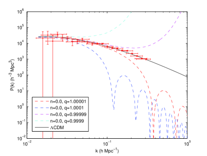
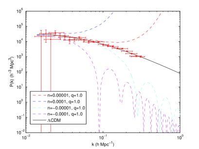
Figure 4: The matter power spectrum in the MPC model without baryons. for small deviation of $q$ (a) and $n$ (b) from the $\Lambda{}CDM$ values of $q=1,\,n=0$. Also shown are data points and error bars from the SDSS project.

From the figures it is clear that the matter power spectrum is drastically modified, much like in the Chaplygin gas scenario studied in [13]. Even a small deviation from the $\Lambda$CDM values ($n=0,\ q=1$) leads to either strong oscillations or growth in the spectrum, depending on the signs of $n$ and $q-1$. This is explained by the non-zero sound speed that seeds the non-standard evolution of $\delta_{m,k}$ due to the $c_{s}^{2}k^{2}/a^{2}$-term in Eq. (4.1). We know generally that perturbations in a comsological fluid with $c_{s}^{2}>0$ will fluctuate for scales smaller than the Jeans length, which is the scale when pressure start to dominate over gravity. While for fluids with $c_{s}^{2}<0$, they will be unstable and grow exponentially for the same scales. A more thorough discussion on perturbations for fluids with non-zero sound speed can be found in [44].

Expanding the sound speed for the MPC model (22) in the small quantities $n$ and $q-1$, we find that they determine the sign of $c_{s}^{2}$. For $n>0$ and $q-1\leq 0$ $c_{s}^{2}$ will be negative and hence give rise to exponentially growing perturbations, while for $n\leq 0$ and $q-1>0$ $c_{s}^{2}$ will be positive and the perturbations will oscillate. This is exactly the behaviour we see in Fig. 4. This behaviour for large $k$ can also be understood directly from Eq. (4.1). In the large $k$ limit we can ignore all but the $k^{2}$ term in the factor that multiplies the zeroth derivative of the density perturbation. Then the differential equation simplifies to

$$\ddot{\delta}_{\rm m,k}+H(2-3c_{s}^{2})\,\dot{\delta}_{\rm m,k}+{c_{s}^{2}k^{2}\over a^{2}}\delta_{\rm m,k}=0\,$$ (23)

We can get a feeling for how the density perturbation behaves in this limit by looking at the case where the time variation of $a$ and $c_{s}^{2}$ is relatively slow. Then both $a$ and $c_{s}^{2}$ will be approximately constant, and the first derivative term in the differential equation will vanish. The differential equation reduces then to the common harmonic oscillator equation, with the following solution

$$\delta_{m,k}(t_{0})\sim e^{-ic_{s}kt_{0}}.$$ (24)

From this we see that a positive $c_{s}^{2}$ will give oscillating perturbations, while a negative $c_{s}^{2}$ gives exponentially growing perturbations. We expect the perturbations to exhibit such behaviour for scales smaller than the Jeans length. The Jeans length is given by the expression

$$\lambda_{J}^{2}\equiv|c_{s}^{2}|\frac{\pi}{G\rho}\,.$$ (25)

For the Cardassian model the Jeans length today can be written as

$$\lambda_{J,0}^{2}=\frac{8\pi^{2}}{3}\frac{n-1}{H_{0}^{2}}\frac{\Omega_{C}}{1+\Omega_{C}}\left(1+\frac{(n-1)q}{1+n\Omega_{C}}\right).$$ (26)

The pressure starts to dominate when

$$k>\frac{2\pi a}{\lambda_{J}}\equiv{k_{J}}$$ (27)

Let us look explicitly at the Cardassian model with parameters $n=0$ and $q=1.00001$. Using the expression for the Jeans length in Eq. (26), we find that $k_{J}\approx 0.6\,$h/Mpc. According to our simplified analysis, the perturbations should then start to grow exponentially when $k>0.6\,$h/Mpc. This agrees fairly well with what we see in Fig. 4a.

In [45] it was argued that the very tight constraints in the Chaplygin case arising from the strong deviations in the matter power spectrum could be relaxed by considering the effect of baryons. Even though the constraints are relaxed slightly, the overall effect is very strong and the fluctuating Chaplygin gas scenario remains tightly constrained [13], even without considering the overall normalization of the spectrum, which tightens the constraints even more. Here, we expect a similar situation to apply but for completeness consider the effect of adding the baryons to the system.

For $k\geq H$ the evolution of linear density perturbations of the Cardassian and the baryon fluids are given approximately by a coupled set of second order differential equations. Taking the equation of state parameter and the adiabatic sound speed of matter to be zero, these differential equations can be written as ([43, 13]):

$$\mbox{$$}\ddot{\delta_{k}}+H\Big{(}2-3(2\omega-c_{s}^{2})\Big{)}\dot{\delta_{k}}-\Big{(}\frac{3}{2}H^{2}(7w-3w^{2}-6c_{s}^{2})-(\frac{c_{s}k}{a})^{2}\Big{)}\delta_{k}$$

$$-\frac{3}{2}H^{2}(1+w)\frac{\rho\delta_{k}+\rho_{b}\delta_{b,k}}{\rho+\rho_{b}}=0$$ (28)

and

$$\ddot{\delta_{b}}+2H\dot{\delta_{b}}-\frac{3}{2}H^{2}\frac{\rho\,\delta+\rho_{b}\delta_{b}}{\rho+\rho_{b}}=0\,,$$ (29)

where $\delta$ is again the density perturbation of the Cardassian fluid, $\delta_{b}$ the density perturbation of the baryon fluid and $w$ and $c_{s}^{2}$ are the equation of state parameter and adiabatic sound speed of the Cardassian fluid.

We solve the equations as before and the resulting matter power spectrum is shown in Fig. 5. We see that adding the baryons to the system does improve the situation as the oscillatory behaviour disappears, and the main effect is a reduction in small-scale power. The constraints are still very strong, but bearing in mind that we have neglected other effects which can result in less power on small scales, e.g. neutrino masses and a scale-dependent bias between matter and galaxy clustering, this simple analysis cannot rule out these models completely. However, as shown in [41], the integrated Sachs-Wolfe effect in the CMB leads to very strong constraints on models with $c_{s}^{2}>0$. In the cases where $c_{s}^{2}<0$, the exponential blow-up is still present, and is strongly disfavoured by the galaxy power spectrum.

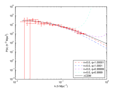
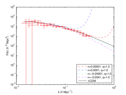
Figure 5: The matter power spectrum in the MPC model with baryons for small deviation of $q$ (a) and $n$ (b) from the $\Lambda{}CDM$ values of $q=1,\,n=0$. The oscillatory behaviour has now vanished for $n<0$ and $q>1$ but still very small deviations from the $\Lambda$CDM model worsen the fit to SDSS data.

Here, considering the effect on $\sigma_{8}$, does not tighten the constraints like in the Chaplygin gas case. This can be seen by comparing how the linear growth is changed in the two scenarios: the Chaplygin gas case is shown in [46] and the MPC case in [24]. Linear growth in the Chaplygin gas scenario changes radically for very small deviations from the parameter values corresponding to the $\Lambda$CDM model, whereas for the MPC model this is not the case. We have checked that this also holds for the parameter values considered here by calculating the linear growth in the MPC scenario for $n<0,\ q<1$. Linear growth is modified, but not as radically as in a Chaplygin gas dominated universe and the LSS constraints are much tighter. Therefore adding baryons gives somewhat more freedom in choosing the parameters in the MPC scenario, but one should bear in mind the strong constraints from the ISW effect [41]. As is clear from Fig. 5, the parameter space is highly constrained and the model offers no good alternative to the $\Lambda$CDM model.

5 Conclusions

We have considered the observational constraints arising from current CMB, SNIa and LSS data on commonly considered models within the Cardassian framework, the original Cardassian model and the Modified Polytropic Cardassian model. Both models were introduced as an alternative explanation to the acceleration of the universe.

Considering that the models only have an effect on the background evolution, CMB and SNIa observations constrain the allowed parameter space. We find that, within the approximation that only background evolution is modified, using the full CMB spectrum constrains the original Cardassian model significantly and that the model offers no advantage over the $\Lambda$CDM model. Adding a new degree of freedom by extending the consideration to the Modified Polytropic Cardassian model relaxes the constraints somewhat but still the parameter space is more constrained than what one finds using the supernovae data only. The constraints indicate that a somewhat non-standard model is slightly preferred over the $\Lambda$CDM model but not significantly.

Viewing the Cardassian models as arising from a interacting fluid constrains the scenario critically. Considering the growth of fluctuations along with the SDSS data, we find that any deviation from the $\Lambda$CDM model is strongly disfavoured, with or without including baryons in the calculation. The fluid interpretation of the Cardassian model is hence effectively excluded as a viable alternative to the $\Lambda$CDM model. This is further supported by recent work [41], where the CMB TT power spectrum in the Cardassian model with fluctuations is demonstrated to be modified strongly on large scales.

In short, even small deviations from the $\Lambda$CDM model within the fluid interpretation of the Cardassian model are strongly disfavoured by current data. If on the other hand, only background evolution is modified, the data indicates a slight preference over the $\Lambda$CDM model but the difference is not significant.

References

References

- [1] Riess A G et al., Observational Evidence from Supernovae for an Accelerating Universe and a Cosmological Constant, 1998 Astron. J. 116 1009 [astro-ph/9805201]
- [2] Perlmutter S. et al., Measurements of Omega and Lambda from 42 High-Redshift Supernovae, 1999 Astrophys. J. 517 565 [astro-ph/9812133]
- [3] Efstathiou G. P. et al., Evidence for a non-zero and a low matter density from a combined analysis of the 2dF Galaxy Redshift Survey and cosmic microwave background anisotropies, 2002 Mon. Not. R. Astron. Soc. 330 L29 [astro-ph/0109152]
- [4] Tegmark M. et al., Cosmological parameters from SDSS and WMAP, 2003 Phys. Rev. D 69 103501 [astro-ph/0310723]
- [5] Tegmark, M. et al.,The Three-Dimensional Power Spectrum of Galaxies from the Sloan Digital Sky Survey, 2004 Astrophys. J. 606 702 [astro-ph/0310725]
- [6] Weinberg S., The cosmological constant problem, 1989 Rev. Mod. Phys. 61 1
- [7] Wetterich C., Cosmology and the fate of dilatation symmetry, 1988 Nucl. Phys. B 302 668
- [8] Peebles P J E and Ratra B., Cosmology with a time-variable cosmological ‘constant’, 1988 Astrophys. J. 325 L17
- [9] Ratra B and Peebles P J E, Cosmological consequences of a rolling homogeneous scalaer field, 1988 Phys. Rev. D 37 3406
- [10] Kamenshchik A. Moschella U and Pasquier V, An alternative to quintessence, 2001 Phys. Lett. B 511 265 [gr-qc/0103004]
- [11] Bilic, N Tupper G B and Viollier R D , Unification of Dark Matter and Dark Energy: the Inhomogeneous Chaplygin Gas, 2001 Phys. Lett. B 535 17 [astro-ph/0111325]
- [12] Bean R and Dore O, Are Chaplygin gases serious contenders to the dark energy throne?, 2003 Phys. Rev. D 68 023515 [astro-ph/0301308]
- [13] Sandvik H, Tegmark M, Zaldarriaga M and Waga I, The end of unified dark matter?, 2004 Phys. Rev. D 69 123524 [astro-ph/0212114]
- [14] Dvali G, Gabadadze G and Porrati M, 4D Gravity on a Brane in 5D Minkowski Space, 2000 Phys.Lett. B 485 208 [hep-th/0005016]
- [15] Deffayet C., Cosmology on a Brane in Minkowski Bulk, 2001 Phys.Lett. B 502 199 [hep-th/010186]
- [16] Deffayet C, Dvali G and Gabadadze G, Accelerated Universe from Gravity Leaking to Extra Dimensions, 2002 Phys. Rev. D 65 044023 [astro-ph/0105068]
- [17] Dvali G and Turner M S, Dark Energy as a Modification of the Friedmann Equation, 2003 Preprint astro-ph/0301510
- [18] Carroll S M, Duvvuri V, Trodden M and Turner M S, Is Cosmic Speed-Up due to new Gravitational Physics?, 2003 Phys. Rev. D 70 043528 [astro-ph/0306438]
- [19] Freese K and Lewis M, Cardassian Expansion: a Model in which the Universe is Flat, Matter Dominated, and Accelerating, 2002 Phys. Lett. B 540 1 [astro-ph/0201229]
- [20] Gondolo P and Freese K, Fluid Interpretation of Cardassian Expansion, 2003 Phys. Rev. D 68 063509 [hep-ph/0209322]
- [21] Elgarøy Ø and Multamäki T, 2004 Preprint astro-ph/0404402
- [22] Chung D and Freese K, Cosmological Challenges in Theories with Extra Dimensions and Remarks on the Horizon Problem, 1999 Phys. Rev. D 61 023511 [hep-ph/9906542]
- [23] Cline J M and Vinet J, Problems with Time-Varying Extra Dimensions or ‘Cardassian Expansion’ as Alternatives to Dark Energy, 2003 Phys. Rev. D 68 025015 [hep-ph/0211284]
- [24] Multamäki T, Gaztañaga E and Manera M, Large scale structure in non-standard cosmologies, 2003 Mon. Not. R. Astron. Soc. 344 761 [astro-ph/0303526]
- [25] Lue A, Scoccimarro R and Starkman G D, Probing Newton’s Constant on Vast Scales: DGP Gravity, Cosmic Acceleration and Large Scale Structure, 2004 Phys. Rev. D 69 124015 [astro-ph/0401515]
- [26] Deffayet C et al. Supernovae, CMB, and gravitational leakage into extra dimensions, 2002, Phys. Rev. D 66 024019 [astro-ph/0201164]
- [27] Barris B J et al., 23 High Redshift Supernovae from the IfA Deep Survey: Doubling the SN Sample at , 2004 Astrophys. J. 602 571 [astro-ph/0310843]
- [28] Hinshaw G et al., First Year Wilkinson Microwave Anisotropy Probe (WMAP) Observations: Angular Power Spectrum, 2003 Astrophys. J. Suppl. Ser. 148 135 [astro-ph/0302218]
- [29] Verde L et al., First Year Wilkinson Microwave Anisotropy Probe (WMAP) Observations: Parameter Estimation Methodology, 2003 Astrophys. J. Suppl. Ser. 148 195 [astro-ph/0302218]
- [30] Seljak U and Zaldarriaga M, A Line of Sight Approach to Cosmic Microwave Background Anisotropies, 1996 Astrophys. J. 469 437 [astro-ph/9603033]
- [31] Freedman W L et al., Final Results from the Hubble Space Telescope Key Project to Measure the Hubble Constant, 2001 Astrophys. J. 553 47 [astro-ph/0012376]
- [32] Frith W J, Constraints on Cardassian Expansion, 2004 Mon. Not. Roy. Astron. Soc. 348 916 [astro-ph/0311211]
- [33] Gong Y and Duan C-K, Supernova constraints on alternative models to dark energy, 2004 Mon. Not. Roy. Astron. Soc. 352 [astro-ph/0401530]
- [34] Sen S and Sen A A, Observational Constraints on Cardassian Expansion, 2003 Astrophys. J. 588 1 [astro-ph/0211634]
- [35] Nesseris S and Perivolaropoulos L, A comparison of cosmological models using recent supernova data, 2004 Phys. Rev. D 70 043531 [astro-ph/0401556]
- [36] Wang Y, Freese K, Gondolo P and Lewis M, Future Type Ia Supernova Data as Tests of Dark Energy from Modified Friedmann Equations, 2003 Astrophys J. 594 25 [astro-ph/0302064]
- [37] Zhu Z-H, Fujimoto M-K and He X-T, Observational constraints on cosmology from modified Friedmann equation, 2004 Astrophys. J. 603 365 [astro-ph/0403228]
- [38] Sen S and Sen A A, WMAP constraints on Cardassian model, 2003 Phys. Rev. D 68 023513 [astro-ph/0303383]
- [39] Zhu Z-H and Fujimoto M-K, Constraints on Cardassian Scenario from the Expansion Turnaround Redshift and the Sunyaev-Zeldovich/X-ray Data, 2004 Astrophys. J. 602 12 [astro-ph/0312022]
- [40] Savage C, Sugiyama N and Freese K, Age of the Universe in the Cardassian Model, 2004 Preprint astro-ph/0403196
- [41] Koivisto T, Kurki-Suonio H and Ravndal F, 2004 Preprint astro-ph/0409163
- [42] Multamäki T and Elgarøy Ø, The Integrated Sachs-Wolfe effect as a probe of non-standard cosmological evolution, 2004, Astron. & Astroph, 423 (2004) 811 [astro-ph/0312534]
- [43] Lyth D and Stewart E, The evolution of density perturbations in the universe, 1990 Astrophys. J. 361 343
- [44] Hu W, Structure formation with generalized dark matter, 1998 Astrophys. J. 506 485
- [45] Beca L M G, Avelino P P, de Carvalho J P M and Martins C J A P, Role of baryons in unified dark matter models, 2003 Phys. Rev. D 67 101301(R) [astro-ph/0303564]
- [46] Multamäki T, Gaztañaga E and Manera M, Large scale structure and the generalised Chaplygin gas as dark energy, 2004, Phys. Rev. D 69 023004 [astro-ph/0307533]