The Rise of the $s$-Process in the Galaxy

Abstract

From newly-obtained high-resolution, high signal-to-noise ratio spectra the abundances of the elements La and Eu have been determined over the stellar metallicity range $-3<$[Fe/H]$<+0.3$ in 159 giant and dwarf stars. Lanthanum is predominantly made by the $s$-process in the solar system, while Eu owes most of its solar system abundance to the $r$-process. The changing ratio of these elements in stars over a wide metallicity range traces the changing contributions of these two processes to the Galactic abundance mix. Large $s$-process abundances can be the result of mass transfer from very evolved stars, so to identify these cases, we also report carbon abundances in our metal-poor stars. Results indicate that the $s$-process may be active as early as [Fe/H]$=-2.6$, alalthough we also find that some stars as metal-rich as [Fe/H]$=-1$ show no strong indication of $s$-process enrichment. There is a significant spread in the level of $s$-process enrichment even at solar metallicity.

1 Introduction

Abundances of elements determined in stars over a very wide metallicity range contain vital clues to the chemical evolution of our Galaxy. This is especially true for the neutron capture ($n$-capture) elements, those heavier than the Fe peak (Z$>$30). Syntheses of $n$-capture elements occur in a variety of fusion episodes in the late stages of stellar evolution, with neutron densities that range over factors of 10¹⁵.

During quiescent He-burning, neutrons generated via the ¹³C($\alpha$,n)¹⁶O and ²²Ne($\alpha$,n)²⁵Mg reactions are captured by heavy element seed nuclei. The neutron densities are relatively low (N${}_{n}\sim$10⁸ cm^-3; Pagel 1997), so nearly all possible $\beta$-decays will have time to occur between successive neutron captures. Synthesis of successively heavier isotopes progresses along the “valley of $\beta$-stability”. This synthesis route is called the $s$-process, and it is responsible for about half of the isotopes of the $n$-capture elements. Much larger neutron densities ($\geq$10²³ cm^-3; Pagel 1997) are generated via p + e $\rightarrow$ n + $\nu$ during the high-mass-star core collapse that results in Type II supernovae (SNe). Extremely neutron rich nuclei are formed in a matter of seconds; in this so-called $r$-process, it is not necessary to have pre-existing heavy-element seed nuclei. The $n$-capture rates exceed $\beta$-decay rates, creating nuclei out to the neutron drip line. These extremely neutron rich nuclei experience multiple $\beta$-decays back to the valley of $\beta$-stability after the very quick extinction of $n$-capture events as the Type II SN envelopes are ejected. The $r$-process is also responsible for about half of the solar system $n$-capture isotopes but not always the same ones created in the $s$-process. Thus, $n$-capture elements can be composed of some pure $r$-process, pure $s$-process, and some mixed-parentage isotopes.

Abundance studies of very low metallicity stars cannot measure isotopic abundances from typical absorption lines; the isotopic wavelength offsets are usually very small compared with other line-broadening effects. The only exceptions for the Z$>$30 elements to date are Eu (Sneden et al., 2002; Aoki et al., 2003) and Ba (Magain, 1995; Lambert & Allende Prieto, 2002). Therefore, to help understand the relative importance of the two $n$-capture synthesis mechanisms throughout the history of the Galaxy, stellar elemental abundance comparisons are made between elements whose solar system isotopic abundances are dominated by the $s$-process and those due mainly to the $r$-process.

Beginning with Spite & Spite (1978), such comparisons have nearly always focused on the relative abundances of Ba (Z=56, $\approx$85% $s$-process in the solar system) and Eu (Z=63, $\approx$97% $r$-process; see Burris et al. 2000 and references therein). The massive stars that are althought to provide the site of the $r$-process evolve on much shorter time scales than the lower mass stars that manufacture $s$-process elements. On the average, then, older stars ought to show a pure or almost pure $r$-process signature (Truran, 1981). While simple in principle, observational evidence for the onset of the $s$-process in a general way is still lacking. A recent and extensive study of $n$-capture elements in metal-poor giant stars by Burris et al. (2000) offers a somewhat inconclusive answer to the question of when low-mass stars begin to contribute to the Galactic chemical mix. They found that the $s$-process may begin to contribute at lower metallicities than expected, an effect somewhat blunted by the considerable range in Ba/Eu abundance ratios at any given metallicity. In contrast, Mashonkina et al. (2003) found that the onset of the $s$-process occurred at higher metallicities and that evolution of the $s$-/$r$-process ratio could be tied to Galactic stellar populations. There is much less variation in the Ba/Eu ratio in the latter study.

Unfortunately, the observational and analytical uncertainties in [Ba/Eu] abundance ratios are substantial and may contribute considerably to the ambiguity of previous results. Often, Ba abundances are derived from just a handful of Ba II transitions (mainly the 4554 Å resonance line, now sometimes accompanied by the 5853, 6141, and 6496 Å lines), and Eu abundances from the Eu II transitions at 4129 and 4205 Å (François, 1996; McWilliam, 1998; Burris et al., 2000). Detailed hyperfine and isotopic substructure analyses have been published for Eu II features along with reliable transition probabilities, so accurate Eu abundances may be routinely determined (Lawler et al., 2001b). Barium abundance uncertainties now dominate the problem. The near-ground-state Ba II lines most commonly measured are usually very strong, while higher excitation lines (at 3891, 4130, and 4166 Å) are almost all undetectable. The low-excitation transitions are often saturated, yielding Ba abundances that are very sensitive to adopted values of stellar microturbulent velocities. In In addition, Ba has five abundant isotopes (¹³⁴Ba-¹³⁸Ba) which are synthesized in different proportions by $r$- and $s$-processes. Therefore, elemental abundances depend on the assumed $r$/$s$ fraction, which is what one is ultimately attempting to determine; these difficulties are especially acute for the 4554 Å line. From these effects, it is difficult to assess the Ba abundances in most stars to better than $\pm$0.2 dex. It is not at all obvious whether observed star-to-star scatter in [Ba/Eu] ratios at a given [Fe/H] metallicity is primarily indicative of astrophysical variations or Ba measurement uncertainties.

Fortunately, neighboring rare earth elements whose solar system abundances are mainly due to the $s$-process may be easily observed in stars over a wide metallicity range. In particular, La (Z=57, $\approx$75% $s$-process in the solar system; Burris et al. 2000) has many detectable features of La II. This species has enjoyed a recent laboratory study that yielded accurate transition probabilities and hyperfine structure constants (Lawler et al., 2001a). There are La II lines of different strength throughout the near-UV to red spectral regions, and all of them yield consistent abundances from the solar spectrum and from $r$-process-rich, low-metallicity stars such as BD +17^∘3248, BPS CS 22892-052, and BPS BPS CS 31082-001 (Lawler et al., 2001a; Sneden et al., 2003; Hill et al., 2002). Finally, ¹³⁹La is the only abundant naturally-occurring isotope of La, so $r$- and $s$-process contribution estimates are irrelevant to the determination of total elemental La abundances (Lodders, 2003).

In this paper we report new La and Eu abundances for 159 giant and dwarf stars. Our aim is to refine measurements of the $s$-/$r$-process ratio to the point where measurement uncertainties no longer obscure the onset of nucleosynthetic contributions from asymptotic giant branch (AGB) stars. Our data also allow us to address $s$-process evolution in the Galactic stellar populations that we have sampled. In §2 we present the spectroscopic data, in §3 we discuss the abundance analyses, in §4 we discuss our results in relation to previous work, and in §5 we discuss the Galactic trend in La/Eu ratios and the relationship between La/Eu and stellar kinematics. Section 6 contains some concluding remarks.

2 Observations and Data Reduction

Stars were initially selected to have $-2.5\leq$[Fe/H]$\leq-1.0$, alalthough our analysis scattered some stars to higher or lower metallicities. Program stars were taken from the objective prism survey of Bond (1980) and the high proper-motion survey of Carney et al. (1994). Our sample therefore includes both main-sequence and evolved stars in roughly equal proportions. There is a weak correlation between evolutionary state and [Fe/H] in our final sample, such that the more metal-poor stars ($-3.0\leq$[Fe/H]$\leq-1.7$) are more likely to be evolved stars and the more metal-rich stars ($-1.2\leq$[Fe/H]$\leq-0.5$) are more likely to be unevolved stars. In order to maintain a high signal-to-noise ratio (S/N) in all our spectra, our program was limited to stars with V$\leq$11. Of the 98 stars observed for this program, 92 proved to have measurable lines of La or Eu or both. A further four dwarf stars were rejected from the sample after having been identified by Latham et al. (2002) as single-lined spectroscopic binaries. The final sample is composed of 88 metal-poor stars.

Spectra of these stars were obtained with the McDonald Observatory 2.7-m telescope, using the “2-d coudé” cross-dispersed echelle spectrograph configured to a 2 pixel resolving power of R$\sim$60,000 and a Tektronix 2048x2048 CCD. This instrument allows full optical wavelength coverage in the blue, alalthough in some cases red spectral features (i.e., the 5797 Å La II or the 6432 Å  Eu II line) were lost off the detector chip and could not be included in our analysis. Most spectra have S/N$\sim$100 pixel^-1 at 4100 Å, with a few cool stars having lower S/N in the blue part of the spectrum (where the majority of measurable La and Eu lines lie). However, cooler stars have deeper lines, which aids the measurement process in these cases.

In addition to the metal-poor stars observed, 67 Galactic disk stars observed by Woolf et al. (1995) were added to our sample. These stars span a higher metallicity range, $-0.85\leq$[Fe/H]$\leq+0.20$, and are all unevolved stars. Stellar parameters from Woolf et al. (1995) have been adopted without changes; the details of those derivations can be found in their paper. The Woolf et al. (1995) study, although conducted with the same telescope and instrument, employed a different CCD chip and instrument configuration. In order to investigate the effects of this and differing analysis methods, we re-observed five stars from the Woolf sample and analyzed them according to the same methods used for the stars in the lower metallicity sample.

Bias subtraction, flat-field corrections, and wavelength calibrations were performed using the standard routines available in IRAF . We used the software package SPECTRE (Fitzpatrick & Sneden, 1987) for the remainder of the stellar data reductions, to eliminate anomalous radiation events and co-add and normalize spectra with spline function fits to interactively chosen continuum points. Spectra of lower quality or cool stars with lower flux in blue portions of the spectra were smoothed by convolving a Gaussian of 2 pixel FWHM with the observed spectra. We also used SPECTRE to measure equivalent widths (EWs) of spectral lines, either by fitting a Gaussian profile to the line or by a simple integration.

3 Analysis

Our abundance analysis is a combination of spectrum synthesis and EW analysis, both of which require a model of the star’s atmosphere. The model atmospheres in turn are characterized by four input parameters: $T_{\rm{eff}}$, log$~{}g$, [Fe/H], and v_t. It is common for these quantities to be derived from Fe I and Fe II EWs. However, we have used other methods to obtain independent estimates of these quantities, which were then checked against the standard spectroscopic constraints. In the following sections we describe our initial estimates of stellar model parameters and the confirmation methods we used to determine final values and elemental abundances. At this point we introduce our summary table, Table 1, which contains initial stellar parameter estimates, final parameters, and the abundance ratios we have ultimately derived.

3.1 Stellar Models

Abundances were derived using Kurucz stellar atmosphere models with no convective overshoot (Castelli et al., 1997). Models were interpolated to a particular set of pre-determined stellar parameters (see next sections) using software provided by A. McWilliam (1990, private communication) and I. Ivans (2002, private communication). For those stars for which model atmosphere parameters were chosen by EW analysis of Fe I and Fe II lines, models were tested in steps of 25 K in $T_{\rm{eff}}$ and 0.25 dex in log $g$.

3.2 Line Lists

3.2.1 Iron

Stellar parameters were checked with EW measurements of a small list of Fe I and Fe II lines. The 11 Fe II and 21 Fe I lines that were selected from Grevesse & Sauval (1999) are listed in Table 2. Since we have sampled a wide range of metallicity and temperature with the same line list, the number of Fe I and Fe II lines used to derive [Fe/H] for a particular star varies as indicated in Table 1.

3.2.2 Lanthanum and Europium

The La II and Eu II transitions measured in this study are also listed in Table 2. The spectral lines of La and Eu both have hyperfine components of varying separation and intensity, which make an EW analysis inappropriate. In addition, Eu has two naturally occurring isotopes that are abundant in approximately equal proportions (Lodders, 2003), further contributing to the broadening of Eu lines (Lawler et al., 2001b; Sneden et al., 2002; Aoki et al., 2003). As mentioned earlier, La has only one abundant naturally occurring isotope. Abundances from strong Eu and La lines cannot be accurately measured by single-line equivalent widths and are therefore more properly obtained by synthesizing the various hyperfine and isotopic components of the lines and fitting the syntheses to the observed spectrum. For the sake of uniformity, we have synthesized all La and Eu lines, even those weak lines usually deemed acceptable for EW analysis. The transitions measured here are taken from those used to measure the solar photospheric abundances in Lawler et al. (2001a, b). Most of the stars in our temperature and metallicity range have at least two measurable Eu II and four or five La II lines. Fewer Eu II lines are typically measurable, as some of the strongest Eu II transitions are often in the wings of very strong absorption features. This is especially a problem with the line at 3819 Å, and, although it is quite strong, an accurate abundance can rarely be easily derived from it. In the Woolf et al. sample, only one line of La and one line of Eu were available for measurement.

We list in Table 3 and Table 4 the abundances derived from each La and Eu line in our metal-poor stars. The final two columns of these tables list the average La or average Eu abundance and the $\sigma$ of each. We use these average values in Table 2 and in our figures.

3.2.3 Carbon

We derived carbon abundances from synthetic spectrum analyses of selected portions of the CH A${}^{2}\Delta-X^{2}$ G band, adopting the atomic and molecular line lists from the Kurucz web site. We synthesized a 30 Å region centered on 4315 Å, stepping the carbon abundance in increments of 0.50 dex. This line list is the one employed by Westin et al. (2000). When used in conjunction with a Kurucz solar no-overshoot model atmosphere, it produces a solar carbon abundance of log$\epsilon$(C)=8.61. We have used this value when calculating [C/Fe] (see Table 1).

3.3 Stellar Parameters

3.3.1 Effective Temperature by Means of the Infrared Flux Method

Effective temperature ($T_{\rm{eff}}$) was determined using the Infrared Flux Method (IRFM) calibrations of Alonso et al. (1996) (dwarf stars) and Alonso et al. (1999) (giant stars). Many program stars have published IRFM temperatures calculated by Alonso et al. with their own measured colors, which we adopt whenever they are consistent with our EW analysis (see next sections). For program stars not observed by Alonso et al., $T_{\rm{eff}}$ was derived using the calibration $V-K$ (chosen because it is especially insensitive to the choice of metallicity). We have used Two Micron All-Sky Survey (2MASS) $K$ magnitudes and Tycho-2 $V$ magnitudes as these were available for all our program stars. However, this raises the possibility of systematic offsets between those temperatures calculated with Alonso et al. (1996, 1999) colors and those calculated with colors from other sources. In order to determine and correct systematic offsets in our derived temperatures, we did the following:

1) We obtained $V$ and $K$ magnitudes for the entire Carney et al. (1994) and Bond (1980) catalogues. The Tycho-II $V$ magnitude was transformed according to

$$V_{J}=V_{T}-0.09*(B_{T}-V_{T})$$

(Høg et al., 2000). The 2MASS $K$ was not transformed onto the standard system, since the correction is smaller than the quoted measurement error for stars in this magnitude range. Colors were corrected with reddenings from Anthony-Twarog & Twarog (1994) when necessary. For nearby (i.e., dwarf) stars, reddening is a negligible effect.

2) $T_{\rm{eff}}$ was derived for all stars with $V-K$ in the range covered by the calibration. The $T_{\rm{eff}}$ calibrations also require an estimate of [Fe/H]. We adopted the metallicities provided by Carney et al. (1994) and Anthony-Twarog & Twarog (1994). Although these were not always consistent with our final measurement of [Fe/H] (see §3.3.4), gross disagreements were few and corrected iteratively when necessary.

3) Our calculated temperatures were compared with those published by Alonso et al. (1996, 1999) for overlapping stars. Alonso et al. (1996) calibrations hold for unevolved stars; the mean offset for high-gravity stars is $-17$ K, in the sense $T_{\rm{eff}}$ (this study)$-$$T_{\rm{eff}}$ (Alonso). For evolved stars, the Alonso et al. (1999) calibrations were used. The mean offset for low-gravity stars is $+30$ K, again in the sense of $T_{\rm{eff}}$ (this study)$-$ $T_{\rm{eff}}$ (Alonso).

4) The mean offsets were applied to the calculated $T_{\rm{eff}}$values of all stars in our program. We note that the mean offsets are quite small and well within the error of the calibrations themselves. Also, for both giant and dwarf stars, $\sigma_{\rm{offset}}\approx 200$K.

3.3.2 Spectroscopic Constraints on Effective Temperature

Stellar effective temperatures can also be derived from spectroscopic constraints: specifically, the requirement that the abundances from individual atomic lines be independent of the excitation potential of the line. This is commonly done (in this temperature and gravity regime) by measuring many EWs of some iron peak element (usually Fe I), as a large number of these lines at various excitation potentials are easily measured at optical wavelengths. Stellar models are tested iteratively, until a set of parameters is found that eliminates any correlation between abundance value and excitation potential for the set of lines.

Individual stars may have, for various reasons, IRFM temperatures that are not in agreement with the spectroscopic constraints typically applied when $T_{\rm{eff}}$ is derived from EWs. In order to identify errors in colors, IRFM $T_{\rm{eff}}$ values were checked with a small list of Fe I lines. This same list, with the addition of Fe II lines, served to verify log $g$ and determine [Fe/H] and stellar microturbulence (v_t) as described in the following sections. In those cases in which a stellar model with an IRFM temperature showed a strong trend in Fe I abundance with excitation potential, the temperature was modified until no trends appeared. Our adopted temperatures, calculated IRFM temperatures, and the Alonso et al. published temperatures are given in Table 1.

3.3.3 Surface Gravity

We have obtained two independent estimates of stellar surface gravity: the so-called “physical gravity”, calculated from the standard relation

$$\rm{log}~{}g_{*}=0.4*(M_{V*}+BC-M_{Bol\odot})+log~{}g_{\odot}+4*log(\frac{T_{eff*}}{T_{eff\odot}})+log(\frac{m_{*}}{m_{\odot}})$$

and a “spectroscopic gravity”, set by requiring that [Fe I/H]=[Fe II/H]. Each method has its drawbacks. The physical gravity is limited by the accuracy of the distance measurement, and tends to be most useful for nearby stars with accurate parallaxes. The spectroscopic method is plagued by the possibility of departures from LTE. Several recent studies have called into question the validity of forcing ionization equilibrium for nearby stars where both methods can be used. Thévenin & Idiart (1999) have suggested that the non-LTE (NLTE) effects on Fe lines in dwarf stars can be severe, resulting in large discrepancies in standard analyses between the derived abundance of [Fe I/H] and [Fe II/H] for very metal-poor stars. The extent of NLTE effects on derived Fe abundances in evolved stars has not yet been determined. Therefore, for those stars with accurate parallaxes, we set log $g$ from the standard relation shown above. The stellar mass, $m_{*}$, is either taken from Carney et al. (1994) (for high-gravity stars) or assumed to be 0.8 $m_{\odot}$ (low-gravity stars), the bolometric correction BC is from Alonso et al. (1995, 1999), and we have adopted 4.75 as the bolometric magnitude (M_Bol) of the Sun. The value of M_V∗ can be derived from

$$\rm{M}_{V*}=\rm{m}_{V}+5-5*\rm{log}(\frac{1}{\pi})-3.2*E(B-V)$$

where $\pi$ was taken from Hipparchos (Perryman et al., 1997).

For the more luminous (and usually more distant) stars, Hipparchos parallaxes are insufficient, since the quoted error is often larger than the measurement itself. In these cases, we have used the distances and reddenings derived from Strömgren colors by Anthony-Twarog & Twarog (1994). There are some cases in which gravities derived from the distances given by Anthony-Twarog & Twarog (1994) do not appear to give sensible results, in that the abundance of Fe derived from Fe I is significantly different from the abundance derived from Fe II (and there is no reason to suppose that this is limited to Fe). In those cases where the abundance difference between [Fe I/H] and [Fe II/H] was large (larger than has yet been attributed to NLTE effects; this is $\sim$ 0.40 dex or more), a new gravity was adopted, chosen by forcing [Fe I/H] and [Fe II/H] into agreement. These cases are likely due to very high reddening values, which would make Anthony-Twarog & Twarog (1994) distances more uncertain.

Some stars are in neither the Hipparchos catalogue nor the Anthony-Twarog & Twarog (1994) work; these are primarily mildly metal-poor dwarfs and subgiants. Whenever it was necessary to force agreement, we accepted the value of log$~{}g$ that put the difference in [Fe I/H] and [Fe II/H] within 2$\sigma$ of the [Fe II/H] abundance. Except for the coolest, most metal-poor stars (for which Fe lines were weak or blended), this amounted to less than 0.3 dex (with one exception: see §3.3.4), and no star had a difference exceeding 0.35 dex. Those stars for which log $g$ was not derived directly from a parallax or distance measurement have been indicated in Table 1.

3.3.4 Metallicity

We have derived stellar metallicities from a small list of Fe I and Fe II lines (see section 3.2.1). Because we have not forced the Fe I and Fe II abundances to agree, there may be some ambiguity as to the actual value of the Fe abundance. In choosing stellar models, the adopted Fe abundance is the mean Fe value, weighted by the number of lines measured. For stars more metal-poor than [Fe/H]$\sim-1$, model metallicities were increased by 0.1-0.25 dex to simulate $\alpha$-enhancements (Fulbright & Kraft, 1999).

On the basis of the work of Thévenin & Idiart (1999), some analyses have adopted [Fe II/H] as the “true” Fe abundance (for stars in the F, G, and K temperature ranges) owing to the smaller influence of NLTE effects on this species and the fact that Fe II is the dominant Fe species. In particular, Kraft & Ivans (2003) adopt this convention and note that although Thévenin & Idiart (1999) attribute some of the discrepancy in Fe I and [Fe II/H] to overionization by UV photons in dwarf stars, the sign of $\Delta$ [Fe/H](=[Fe I/H]$-$[Fe II/H]) in giant stars is not always consistent with this. According to Thévenin & Idiart (1999), the derived abundance of Fe II should be consistently higher than that of Fe I, but Kraft & Ivans (2003) have found that this is not necessarily the case. Kraft & Ivans (2003) attribute this to the failure of one-dimensional LTE model atmospheres to accurately represent the abundance of Fe I.

By setting log$~{}g$ from distance measurements, we have largely avoided this issue. However, we do find that there is a systematic offset in $\Delta$ [Fe/H] that is most strongly dependent on $T_{\rm{eff}}$. In Fig. 1 we plot the difference in Fe as measured from [Fe I/H] and [Fe II/H]. At low temperatures, the derived [Fe I/H] is as much as 0.30 dex lower than the derived [Fe II/H]. The difference (on average) effectively disappears for stars with $T_{\rm{eff}}$$>5200$ K, although even at higher temperatures there are individual stars with large $\Delta$ [Fe/H]. Thévenin & Idiart (1999) found that the more metal-poor stars tended to have larger disagreements in $\Delta$ [Fe/H], although there were temperature dependencies as well. While it is tempting to attribute these trends solely to temperature effects, the coolest stars are almost all giants stars and it is at these temperatures that we see trends in $\Delta$[Fe/H]. We can not therefore conclusively distinguish either $T_{\rm{eff}}$ or log $g$ as the controlling variable. It is also not clear that the same mechanism is responsible for the discrepancies in the dwarf stars in Thévenin & Idiart (1999) and the giant stars studied here. We note that Yong et al. (2003) found that metal-poor globular cluster stars showed a similar behavior in $T_{\rm{eff}}$, with $\Delta$ [Fe/H] becoming more pronounced in the coolest giant stars.

With our Fe line list and for $T_{\rm{eff}}$=5780 K, log $g$=4.45, and v_t=0.90 km/s, we derive $\Delta$[Fe/H]=0 in the Sun. However, Fig. 1 reveals that we ought not to expect anything different for those parameters. One star in particular stands out in this figure, the dwarf star HD 188510. It has almost the largest $\Delta$ [Fe/H] (+0.3 dex) in our sample, yet it also has a well-determined Hipparchos parallax ($\pi=25.17$ mas). While this star is at the high $T_{\rm{eff}}$, high log$~{}g$ end of our sample, other stars with similar parameters have a much smaller $\Delta$ [Fe/H]. This star does not appear to be unusual in any other respect, and Latham et al. (2002) does not identify this star as a binary. There is, however, a significant difference in the $K$ magnitudes reported by 2MASS and and that of Alonso et al. (1996). 2MASS finds $K$=7.854 (V-K=1.62) and Alonso et al. use $K$=7.13 (V-K=1.69). The value of Alonso et al. makes the star 200 K hotter than the 2MASS colors would imply, and the lower temperature results in a higher metallicity overall (and a smaller $\Delta$ [Fe/H]). However, our methods find that both temperatures are acceptable for this star, and we have adopted the published Alonso value whenever possible for consistency. We do not find any significant offset in K between Alonso et al. and 2MASS, but values for individual stars may vary. However, La/Eu is not affected by Fe uncertainties of this magnitude (see §3.4).

We have chosen to use [Fe II/H] in most of our figures and in our analysis discussions, mainly because we have measured La II and Eu II. However, our conclusions are not altered by this choice; trends in La/Eu and [Fe I/H] are very similar. We report both [Fe I/H] and [Fe II/H] in Table 1.

3.3.5 Microturbulence

The microturbulence was set by requiring that the derived Fe abundance be independent of the quantity log $(EW/\lambda)$. Derived values of v_t less than $\sim 0.40~{}$km/s were not accepted, as this is equal to a typical error on derived velocity shifts in our spectra. Generally, more Fe I lines are measurable, and they cover a wider range in $(EW/\lambda)$ than the measured Fe II lines. For this reason, the microturbulence derived from Fe I was given more weight whenever mild disagreements arose.

3.3.6 M_V

The majority of the dwarf stars have good Hipparchos parallaxes, and for these stars M_V can be found from the standard relation given in §3.3.3 (for stars within $\approx$1 kpc, reddening was ignored). Anthony-Twarog & Twarog (1994) report M_V for the stars for which they derived reddenings. As these giant stars, while luminous, are generally very distant and have poorly determined parallaxes, the Twarog & Twarog value of M_V was adopted wherever it did not conflict with the log$~{}g$ implied by our Fe line list. The remaining stars have no reliable distance measurement, so an M_V was inferred from the adopted stellar parameters–we simply invert the relation in §3.3.3 to recover M_V. While $T_{\rm{eff}}$ for these stars may be set either from Fe lines or from the IRFM, log$~{}g$ must be set from Fe lines. This method of model selection is less precise and the error in the implied M_V is much greater than for those stars with distance measurements.

Our sample covers a wide range of evolutionary states, from unevolved stars on the main sequence to red giants, as shown in Fig. 2. Behr (2003) identified seven of our sample stars as horizontal branch (HB) stars (HD 025532, HD 082590, HD 105546, HD 166161, HD 119516, HD 184266, and HD 214362). These stars are boxed in Fig. 2.

3.3.7 Kinematics Calculations

The majority of our stars (even the evolved stars) have proper motions available from the Tycho-2 catalogue. Radial velocity measurements were obtained through the SIMBAD database. Most of the bright, nearby dwarf stars have Hipparchos parallaxes, but many of the evolved stars in the sample are too distant to have good measurements. For these stars, we use the “implied” distance from $T_{\rm{eff}}$ and log$~{}g$, as described in §3.4.2. Stars with “implied” distances will necessarily have larger errors in their kinematics (see §3.4.3).

With this information, we have computed the stellar velocities $U$, $V$, and $W$ according to Johnson & Soderblom (1987). Johnson & Soderblom (1987) adopt a right-handed coordinate system, where $U$ (motion radial to the Galactic Center) is defined as positive away from the GC, $V$ (orbital motion around the GC) is defined as positive counter-clockwise, and $W$ (motion in and out of the plane of the disk) is defined as positive northward. Our values and errors are given for all the stars in our sample in Table 5. The velocities listed have been corrected for the solar motion (U$-9$,V$+12$,W$+7$;Mihalas & Routly 1968).

3.4 Error Analysis

3.4.1 Stellar Parameters

Uncertainties in the stellar model parameters may directly affect other derived stellar parameters, as in the case of $T_{\rm{eff}}$ and log$~{}g$. Other effects may be more subtle, and errors in each stellar input parameter can propagate through to affect the final elemental abundance. We find that the particular element ratio La/Eu is insensitive to these uncertainties, and we illustrate this with the following examples.

For the typical giant star HD 105546, a change of $\pm$100 K in $T_{\rm{eff}}$ (a $\sim 2\sigma$ error in the Alonso et al. (1996, 1999) calibrations) produces a change in the calculated log$~{}g$ of $\pm$0.04 dex, resulting in a cumulative change of $\pm 0.10$ dex in [Fe I/H], an $\mp 0.02$ dex in [Fe II/H], and an increase of 0.20 km/s in the chosen value of v_t. In this particular star, the change in log$~{}g$ increased the difference between [Fe I/H] and [Fe II/H]. Cooler stars show a larger change in log$~{}g$, reaching $\pm 0.1$ dex for $T_{\rm{eff}}$$\approx 4000$K. For HD 105546, a change of +100 K in $T_{\rm{eff}}$ and 0.04 dex in log$~{}g$, along with the corresponding changes in [Fe/H] (+0.06 dex) and v_t(+0.20 km/s), produce +0.05 dex change in log$~{}\epsilon$(La II) and +0.06 dex change in log$~{}\epsilon$(Eu II), which is a $-0.01$ dex change in log$~{}\epsilon$(La/Eu). For the dwarf star G102-020 (at similar $T_{\rm{eff}}$ and [Fe/H]), an increase of +100K in $T_{\rm{eff}}$ and +0.03 dex in log$~{}g$ gave almost identical results, making [Fe/H] +0.05 dex larger (a change of +0.08 and $-0.02$ dex in [Fe I/H] and [Fe II/H], respectively). The result was an increase in both log$~{}\epsilon$(La II) and log$~{}\epsilon$(Eu II) of +0.05 dex, making no change in log$~{}\epsilon$(La/Eu).

For those stars for which distance estimates were unreliable, unavailable, or that produced a log$~{}g$ inconsistent with the $\Delta$ [Fe/H] we require, log$~{}g$ was tested in 0.25 dex increments. An increase in log$~{}g$ of this magnitude (again for HD 105546, and keeping $T_{\rm{eff}}$ constant) drives [Fe II/H] +0.10 dex higher while leaving [Fe I/H] unchanged. This alters the average [Fe/H] very little, only +0.03 dex–well within the line-to-line spread of each ion. Our choice of v_t is unchanged. The cumulative changes increase log$~{}\epsilon$(La II) by 0.09 dex and log$~{}\epsilon$(Eu II) by 0.11 dex, decreasing log$~{}\epsilon$(La/Eu) overall by 0.02 dex. For those stars with an IRFM $T_{\rm{eff}}$ inconsistent with our EW Fe analysis, $T_{\rm{eff}}$ was tested in increments of 25 K, which produces negligible changes in log$~{}g$ and [Fe/H]. The result was small changes in log$~{}\epsilon$(La II) and log$~{}\epsilon$(Eu II).

Our Fe line list is not extensive and NLTE effects have not been accounted for, so it is unlikely that the errors in stellar parameters are as small as those investigated in this section. Our parameters are internally consistent to $\Delta\mbox{$T_{\rm{eff}}$}=\pm$100 K (the difference in $T_{\rm{eff}}$ at which trends in excitation potential cannot be reasonably corrected by a different choice of v_t) and $\Delta$ log$~{}g=\pm$0.25 dex (the difference in log$~{}g$ at which [Fe II/H] changes by 1 $\sigma_{[Fe~{}II/H]}$), and $\Delta$ v_t=$\pm$0.1 km/s (the difference in v_tfor which a correlation in [Fe I/H] as a function of log (EW/$\lambda$) appears). Note that the cumulative change in the calculated log$~{}g$ arising from a 100 K change in $T_{\rm{eff}}$ and 10% changes in the assumed mass, M_V, and BC_V is smaller, $\approx 0.1$ dex (for stars with $T_{\rm{eff}}$ $\geq$ 5200 K; in cooler stars the calculated log$~{}g$ is more sensitive to changes in $T_{\rm{eff}}$). Errors in [Fe/H] vary according to the number of measurable [Fe I/H] and [Fe II/H] lines (see Table 1). Typically, $\sigma_{[Fe~{}I/H]}=0.07$ dex and $\sigma_{[Fe~{}II/H]}=0.13$ dex.

3.4.2 Absolute Magnitude and Distance

Some stars (mainly giant and sub-giant stars) have poorly determined distances. Distance and $M_{V}$ can be inferred from stellar parameters chosen with an EW analysis, but then small errors in the input values affect the final answer. $M_{V}$ depends on $T_{\rm{eff}}$, $m_{*}$, log$~{}g$, and the BC. In order to discern the effect of typical errors in these parameters on $M_{V}$, we make the following changes: $\mbox{$T_{\rm{eff}}$}-100$ K, $m_{*}-0.1m_{\odot}$, BC$-0.01$ mag, and log$~{}g+0.25$ dex. This produces a cumulative change in $M_{V}$ of $\sim$+0.9 mag. Reversing the sense of the input errors produces a change in $M_{V}$ of similar magnitude but opposite sign.

The effect of input errors on the derived distance is much greater, and depends also on the adopted reddening, $A_{V}$ (from Schlegel et al. 1998), and the apparent magnitude m_V, which we change by +0.05 mag and –0.1 mag to maximize the change in the distance. The value of the cumulative change in the distance varies widely, but is typically $\sim 40-50\%$ of the original value. Ultimately, we make use of the implied distance in §5.4.1, when we deal with space velocities, and there only the absolute error is relevant to our purposes (we reject stars with velocity errors greater than 100 km/s, an error that may arise from sources other than the distance). Nevertheless, this ensures that the adopted stellar parameters and adopted stellar velocities are self-consistent.

3.4.3 Kinematics

Each of the input quantities carries an error that propagates through the velocity calculations. For stars with implied distances, errors are calculated by propagating errors in individual quantities as described in §3.4.2, with the addition of quoted errors in proper motion (from Tycho-2) and radial velocity (typically 1-2 km/s, taken from SIMBAD). As with $M_{V}$, errors are not entirely symmetric, and we have chosen to adopt the larger error. Although we ultimately eliminate stars with greather than 100 km/s errors in any of the three velocity components, the inclusion of stars with implied distances greatly enlarges our sample.

3.4.4 Carbon

Difficulties inherent in synthesizing large stretches of a spectrum (continuum placement, incomplete or inconsistent line lists, saturated features, etc.) limit the precision of our C abundances (although there is some gain in fitting so many features at once). Fitting errors amount to $\pm 0.1$ dex. In addition, we are inferring the C abundance from molecular features that may be quite sensitive to $T_{\rm{eff}}$ and log$~{}g$ changes. However, our focus in this work is the relative abundances of La and Eu. The C abundances we measure serve only to identify specific cases where unusual pollution (i.e., from a more evolved binary companion) may have occurred. For this we do not require high precision or accuracy, since more detailed and comprehensive C studies (e.g., Kraft et al. 1982; Gratton et al. 2000) find that enhancements of this kind are significant: [C/Fe]$\sim$1.0 dex for BD$-01^{\circ}2582$, a well-known CH giant. Nevertheless, we have re-identified this and other known CH stars (see §5.3.1). Our abundances are generally in good agreement with both Kraft et al. (1982) and Gratton et al. (2000), with average [C/Fe] offsets of +0.18 dex ($\sigma=0.24$) and +0.06 dex ($\sigma=0.16$), respectively.

3.4.5 Lanthanum and Europium

As evidenced in the preceding sections, errors in stellar parameters have virtually no effect on the measurement of log$~{}\epsilon$(La/Eu). Values of log$~{}\epsilon$(La II) and log$~{}\epsilon$(Eu II) are sensitive to stellar parameters, log$~{}g$ most especially, but changes in the model atmosphere choice affect only the absolute measurement of these abundances. The relative abundance of La and Eu is constant so long as the stellar parameters are obtained in a self-consistent manner.

Quoted error bars in La/Eu are

$$\sigma_{La/Eu}=\sqrt{\sigma_{La}^{2}+\sigma_{Eu}^{2}}$$

. This represents the line to line spread in derived abundances–the line measurement error. Deviations between the observed and synthesized spectrum are very typically $\pm$0.05 dex–this is the accumulated error in continuum fitting, wavelength centering, line profile fitting, etc. We therefore take $\pm$ 0.1 dex as the (2$\sigma$) fitting error of a single line. Ultimately, however, if only one line is measurable in a star, that line is very likely to be either weak or blended, and the fitting error may be larger. Since La II and Eu II have similar ionization potentials, the transitions used here have similar excitation potentials, and the structure of the La and Eu atoms are similar, changes in stellar parameters tend to alter log$~{}\epsilon$(La) and log$~{}\epsilon$(Eu II) in concert; these abundances move in the same direction and by almost the same amount in an LTE analysis.

The uncertainties on the log(gf) values of the strong blue lines of La II and Eu II in Table 2 are generally $\pm$ 0.02 dex or 5% with high confidence, because these uncertainties are dominated by the uncertainties of the laser induced fluorescence (LIF) radiative lifetime measurements. The accuracy of LIF radiative lifetime measurements is well documented by multiple comparisons with independent LIF measurements (Table 1 in Lawler et al. 2001a & b) and with regular re-measurement of benchmark lifetimes using the exact same apparatus and procedure (Section 2 in Lawler et al. 2001a & b). The log(gf) of the weak red lines in Table 2 do have larger uncertainties, typically $\pm$ 0.04 dex or 10%, because these uncertainties are dominated by the uncertainties of branching fraction measurements for widely separated lines. In metal-poor stars where spectral features are weak, La and Eu abundances were measured predominantly from the stronger blue lines. In the coolest metal-rich stars, our measurements came mainly from the less saturated red lines. Despite the intrinsic errors in log $gf$, Lawler et al. (2001a & b) found that red and blue lines alike gave the same solar abundance. We have found that that holds true for stars in which all our lines were measurable.

4 Comparison With previous studies

The most recent and comprehensive measurements of $n$-capture elements are those of Burris et al. (2000), which encompassed 70 metal-poor giant stars, many of which are included in our sample. In addition, Johnson (2002) conducted an extensive abundance analysis of several of our most metal-poor stars. Three elements are common to all three studies and of interest here: La, Eu, and Fe.

There is only a small offset between [Fe II/H] values derived in this study and those found in Burris et al. (2000) and Johnson (2002), as shown in Fig. 3. On average, our [Fe II/H] values are larger than those of both Johnson (2002) and Burris et al. (2000): [Fe II/H] (this study)$-$[Fe II/H](Johnson)=0.16 dex and [Fe II/H] (this study)$-$[Fe II/H](Burris)=0.04 dex. The [Fe I/H] values we derive are, on average, smaller than those of Burris et al. (2000) but slightly larger than those found in Johnson (2002): [Fe I/H] (this study)$-$[Fe I/H](Johnson)=0.03 dex and [Fe I/H] (this study)$-$[Fe I/H](Burris)=$-0.08$ dex. These offsets appear to be constant over the range of metallicities sampled and are well within our line-to-line abundance spreads for our stars ($\sigma_{[Fe~{}I/H]}\approx 0.07$ dex and $\sigma_{[Fe~{}II/H]}\approx 0.13$ dex, typically).

In 27 of their stars Burris et al. (2000) were able to measure only Ba, and at that time the improved atomic parameters of Lawler et al. (2001a) and Lawler et al. (2001b) were not available. Despite this (and given allowances for errors on the Burris et al. 2000 measurements), there is a fairly good agreement between the log$~{}\epsilon$(La II) and log$~{}\epsilon$(Eu II) derived in that study and this one, as shown for La (Fig. 4), Eu (Fig. 5), and La/Eu (Fig. 6). This agreement can be attributed to two factors: (1), that Burris et al. (2000) find very similar stellar parameters to ours (one notable exception is HD 171496, the outlier in Figs. 4 and 5, for which Burris et al. (2000) finds a $T_{\rm{eff}}$ 300K cooler) and log$~{}\epsilon$ (X) is sensitive to this where [X/Fe] is not and (2), that Burris et al. (2000) had lower quality spectra and necessarily report La and Eu in stars where these elements are easily measured.

Johnson (2002) also measured $n$-capture elements in a sample of metal-poor stars, and we find here an offset in both La and Eu (see Fig. 4 and Fig. 5). However, log$~{}\epsilon$(La/Eu) is, on the average, quite similar in our study and theirs (see Fig. 6). It should be noted that in some cases–most particularly HD 122563–our log$~{}\epsilon$(La/Eu) is significantly different.

For this star, our values of La and Eu differ from not only Burris et al. (2000) and Johnson (2002), but also Westin et al. (2000). Variances in log$~{}\epsilon$(La II) and log$~{}\epsilon$(Eu II) are to be expected with variances in $T_{\rm{eff}}$ and log$~{}g$, however, log$~{}\epsilon$(La/Eu) might well be expected to be consistent (see §3.4). This is not the case for HD 122563–values of log$~{}\epsilon$(La/Eu) range from 0.41 (Johnson, 2002) to 0.37 (Westin et al., 2000) to 0.30 (Burris et al., 2000). Our adopted log$~{}\epsilon$(La/Eu)=0.24 is the lowest reported among these studies. Interestingly, the log$~{}\epsilon$(La II) we find is quite similar to that measured by Westin et al. (2000) and Burris et al. (2000), with log$~{}\epsilon$(La II)=$-2.20,-2.22,$ and$-2.20$, respectively. The value given by Johnson (2002) is different, log$~{}\epsilon$(La II)=$-2.44$, a change likely due to the very much lower surface gravity adopted there (compare log$~{}g=0.50$, Johnson 2002, with log$~{}g\approx 1.4$ Westin et al. 2000; Burris et al. 2000, and this study). The discrepancies in log$~{}\epsilon$(La/Eu) are therefore due to log$~{}\epsilon$(Eu II), and the source of these discrepancies is not easily explained. We find a higher metallicity for HD 122563 than any of the other three studies (which all use [Fe/H]$=-2.70$) although our $T_{\rm{eff}}$ and log$~{}g$ are comparable (with the exception of Johnson 2002, whose difference in adopted log$~{}g$ is much larger than the difference in adopted $T_{\rm{eff}}$ would indicate). Burris et al. (2000) measure two Eu II lines also used here, the 4129 and 4205 Å lines. Westin et al. (2000) use five lines, three of which (3724, 3930, and 3971 Å) are located in the wings of very strong absorption features (Ca II H and K and a Fe I line), and this very probably affects the abundances derived from them.

The particular case of HD 122563 can serve as an illustration of the general situation: one of the main differences between this study and previous work is not simply the quality of atomic parameters for individual lines, but also the number of lines we have been able to measure in a particular star. Eu II lines are often contaminated by the presence of strong nearby lines, but in many stars we have been able to obtain multiple independent measurements of both Eu II and La II.

Much of our data on La/Eu at near-solar metallicities is from the Woolf et al. (1995) spectra. We find that log$~{}g$ as derived from Hipparchos parallaxes tend to be significantly smaller than those used by Woolf et al. (1995), originally from Edvardsson et al. (1993) (on average our log$~{}g$ is 0.27 dex smaller; only in HR 235 have we reproduced their answer), so much so that we find that $\Delta$ [Fe/H] is positive in each star but one, HR 8354 (see Table 6). On the average, we find that [Fe I/H] is 0.06 dex smaller ($\sigma_{[FeI/H]}=0.11$ dex) and [Fe II/H] is 0.16 dex smaller ($\sigma_{[FeII/H]}=0.11$ dex) when our spectra and analysis methods are used. While there are significant offsets in La II and Eu II ($-0.13$ and $-0.16$ dex, respectively; see Tables 7 and 8 for the line-by-line abundances), the net effect is only a small positive offset in log$\epsilon$(La/Eu) ( such that the La/Eu measured from our spectra is 0.03 dex larger on average). This appears to be independent of metallicity (although we do find a rather lower metallicity for HR 458 than did Woolf et al. 1995). We have added these corrections to the Fe, La, and Eu abundances listed in Table 9 (derived from Woolf et al. spectra), and in all the figures we use the altered values.

5 Results

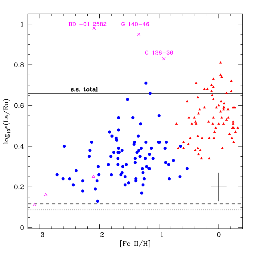
Figure 7: log$\epsilon$(La/Eu) as a function of [Fe/H]. The solid line is the total solar system La/Eu ratio (from Lodders 2003). The broken lines indicate the solar system $s$- and $r$-process abundance breakdowns (see text for descriptions), where the dotted line is from Burris et al. (2000) and the dashed line is from Arlandini et al. (1999). Three metal-poor but La-rich stars are labeled. Symbols are as follows: circles, this study; filled triangles, Woolf et al. (1995); open triangles, three $r$-process enhanced stars (BPS CS 31082-001 Hill et al. 2002, BD +17^∘3248 Cowan et al. 2002b, and BPS CS 22892-052 Sneden et al. 2003); crosses, $s$-process enhanced stars. A typical error is shown.

Our main purpose was to determine at what metallicity the $s$-process begins to contribute significantly to the Galactic chemical mix. That is, to discover at what point low- and intermediate-mass stars start to contribute their nucleosynthetic products and how soon those products dominate. The abundance distributions of the lowest metallicity stars ought to reflect the earliest Galactic nucleosynthesis processes, as these stars were formed from gas that had undergone very little enrichment. In the oldest stars, the abundance pattern might be dominated by the $r$-process, since the high mass stars with which the $r$-process is associated evolve on shorter time scales than the lower mass stars that house the $s$-process (and therefore contribute to the Galactic mix sooner, e.g., Truran 1981). In a general way, we can use the iron abundance of a star as an indication of its formation age (that is, low [Fe/H] stars are older than solar-metallicity stars), and so we plot in Fig. 7 the La/Eu ratio as a function of “time”. Interestingly, this figure suggests that there is no unambiguous value of [Fe/H] at which the $s$-process begins. Not only is there considerable scatter even near solar metallicities (with stars at [Fe/H]$\simeq-0.6$ and log$~{}\epsilon$(La/Eu)$\simeq 0.25$ (a decidedly non-solar value), but at low metallicities ([Fe/H]$<-2$) we find stars with log$~{}\epsilon$(La/Eu)$\simeq 0.4$, nearly 0.20 dex higher than other stars at that metallicity, and few of our metal-poor stars have abundances consistent with a “pure $r$-process” distribution. Although there is an overall upward trend with [Fe/H], at any particular [Fe/H] larger than $\simeq-2$ we find stars with very different La/Eu ratios. These differences are larger than the abundance uncertainties, and we explore interpretations in the next sections.

5.1 Setting the Baseline: The $s$-and $r$-Process at Low Metallicity

The question of when the $s$-process becomes a significant nucleosynthetic contributor can only be reasonably answered if we can probe the time before, when the $r$-process might have dominated heavy element production. For this purpose we again use [Fe/H] as a measure of time and return to Fig. 7, where we have superimposed two horizontal lines - the first is a dotted line indicating the pure $r$-process log(La/Eu) ratio of 0.09 given by Burris et al. (2000). Also shown as a dashed line is a very recent prediction for this $r$-process ratio of 0.12 based upon the Arlandini et al. (1999) stellar model calculations and new experimental cross-section measurements on ¹³⁹La from O’Brien et al. (2003). Some stars at the very lowest metallicities, [Fe/H] $\simeq$ –3, have La/Eu ratios that seem to be consistent with a pure $r$-process origin. Thus, for example, log $\epsilon$(La/Eu) = 0.11 in BPS CS 22892-052 (Sneden et al., 2003), consistent with the new values determined by O’Brien et al. Nevertheless, there is significant scatter in the data at all [Fe/H]. A number of the La/Eu ratios, even for some low-metallicity stars below –2.5, fall above both the O’Brien et al. and Arlandini et al. predictions for pure $r$-process synthesis. Abundance errors are highly unlikely to produce systematically higher La/Eu ratios in such a fashion, and we note that we have employed the same line list as that used for BPS CS 22892-052 (which reproduces the $r$-process value; see Sneden et al. 2003). Interestingly, the older (larger) value for the La cross section as reported in Arlandini et al. 1999 leads to the larger predicted pure $r$-process ratio of 0.26, which would appear to be more consistent with much of the lower metallicity stellar data.

An alternate explanation of these data is that there is some $s$-process synthesis contributing to the La production, even at very low metallicities. Some very low-metallicity stars, such as BPS CS 22892-052 (Sneden et al., 2003), have heavy element abundance patterns that are consistent with the scaled solar system $r$-process curve. It is possible, however, that other low-metallicity stars have been “dusted” with a small $s$-process contribution that might have slightly increased the La value above the pure $r$-process value. (Recall that Eu is almost totally an $r$-process element, while La is mostly produced in the $s$-process in solar system material; see the Appendix.)

Burris et al. (2000) found some indications of $s$-process production in stars even at metallicities as low as [Fe/H] = –2.75, with the more significant processing appearing closer to a metallicity of [Fe/H] = $\simeq$ –2.3. These new abundance data seem to be consistent with those conclusions, and may offer some clues about when, and in what types of stars, the $s$-process occurs. They might, for example, suggest that there is a somewhat wide stellar mass range for the sites of the $s$-process, encompassing more massive intermediate-mass stars with shorter evolutionary times than the main low-mass, slower evolving sites (Travaglio et al., 1999).

5.2 The Abundance Spread

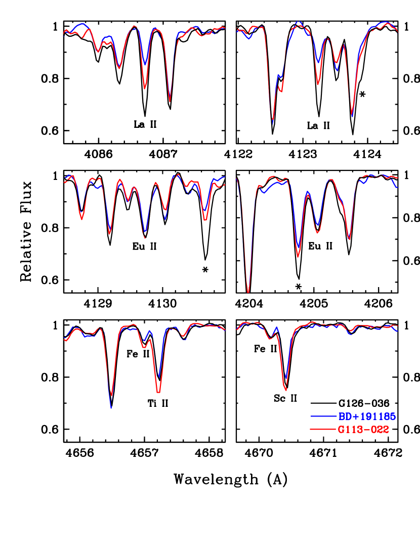
Figure 8: Three stars with identical stellar parameters but very different La abundances. Other $s$-process element features are marked with an asterisk (*).

Despite the overall slow rise, the spread in log$~{}\epsilon$(La/Eu) is significant across almost the entire range in metallicity, and perhaps becomes even larger near solar metallicities. Near [Fe/H]$\simeq-1$, the differences in log$~{}\epsilon$(La/Eu) are real. In at least one case, this difference is due almost exclusively to the varying influence of the $s$-process. In Figure 8, we show three stars with essentially identical stellar parameters, BD $+19^{\circ}$1185A, G 113-022, and G 126-036. From Fig. 7 it is apparent that G126-036 has the highest La/Eu ratio at that metallicity. BD$+19^{\circ}$ 1185A has one of the lowest La/Eu ratios, and G 113-022 falls between them (however, this star still has a higher ratio than the majority of stars in the sample). Since these stars are all at the same $T_{\rm{eff}}$, log$~{}g$, and metallicity, a simple inspection of the spectra may reveal abundance differences. In Fig. 8, it is evident that the depths of the Eu II lines match very well in all three stars, as do other singly-ionized atomic features (Ti II, Fe II, and Sc II are marked). In contrast, the depths of the La II lines are quite different, in the sense that the lines in G126-36 are the strongest, and the lines in BD $+19^{\circ}$1185A are the weakest. Also, the abundance variations are not restricted to La; neighboring features show that several $s$-process elements (marked with asterisks) change in concert with La, and in the same sense. There are other examples of this in our sample, although at very low metallicities the paucity of stars makes it difficult to find parameter pairs. Nevertheless, it is clear that the abundance of $s$-process products at a given metallicity is not single-valued, and can cover a significant range.

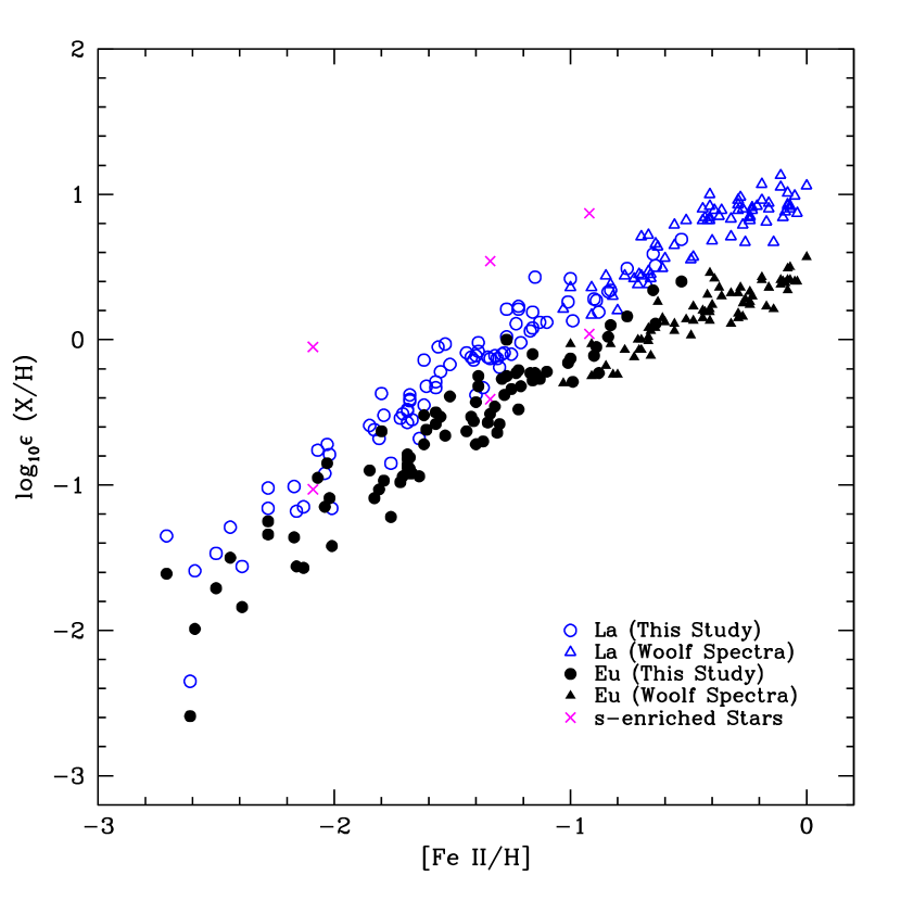
Figure 9: La (open symbols) and Eu (filled symbols) separately. The “$s$-enhanced” stars are marked.

While the case for those three stars is quite clear, we find no evidence that the $s$-process alone contributes to the scatter in La/Eu. In Fig. 9, we plot log$\epsilon$ (La II) and log$\epsilon$ (Eu II) separately as functions of [Fe II/H]. The lowest metallicity stars show widely varying amounts of La II and Eu II (although their ratio is roughly constant); however, the dispersion in each is constant with [Fe II/H]. There is no indication that there is intrinsically more spread in either the $s$-process or $r$-process products at a given iron abundance. As an example, we take the two stars G 102-027 and HR 0033. While these two stars are not similar enough in temperature for their spectra to be visually compared, they have the same overall metallicity ([Fe II/H]$\simeq-0.55$). They also have the same La abundance, log$\epsilon$ (La II)$\simeq$ 0.66. However, G 102-027 has a log $\epsilon$ Eu abundance more than 0.3 dex higher than that of HR 0033 (0.40 dex and 0.06 dex, respectively). The star HR 4039 also has a low Eu abundance at that metallicity (0.08 dex). In fact, at high metallicities we find a spread in Eu that is entirely consistent with that reported by Reddy et al. (2003) for the thin disk–even as other elements (most notably, the iron-peak elements) are virtually single-valued. In addition, our Eu scatter is consistent with the combined thick disk and thin disk population Eu abundances derived by Mashonkina & Gehren (2001), as well as the abundances found by Woolf et al. (1995) (for their total sample). The implication is that that $s$- and $r$-process products are incompletely mixed to a very similar degree even in younger stars.

The overall abundance scatter might point to an early chemically unmixed Galaxy at low metallicity or stellar population contamination at high metallicity, discussed further in the following sections. However, we emphasize the important overall abundance trend –while there is considerable scatter, the La/Eu ratios seem to show a generally rising abundance trend, with increasing Galactic $s$-processing, as a function of metallicity. Despite low ratios in some mildly metal-poor stars, the average log$\epsilon$(La/Eu) does increase with increasing metallicity. These data are consistent with a gradual and continually increasing synthesis in the Galaxy, rather than an abrupt turn-on of the $s$-process.

5.3 The $s$-enhanced Stars

Three metal-poor stars in our sample have very large (super-solar) La/Eu abundance ratios. These stars, BD $-01^{\circ}2582$, G 140-046, and G 126-036, are not representative of the general Galactic trend. All show substantially increased log$~{}\epsilon$(La II) relative to other stars at the same [Fe/H] (see Fig. 9) as well. That these stars differ from the other stars in our sample is also apparent in Fig. 10, where they share a quadrant with the lead stars–stars in which $s$-process enhancements are confirmed by a measurable overabundance of lead (Aoki et al., 2002). These three stars are overabundant in La for their [Eu/Fe] (we also note in Fig. 10 HD 122563, which is curiously Eu-poor).

5.3.1 Carbon Abundances

The $s$-process operates in AGB stars and a particular star’s abundances may simply reflect local pollution. Unusually high $s$-process abundances may also be the result of mass accretion from a more evolved (and now unseen) binary companion. Carbon abundances were measured for our metal-poor stars, and we have compared stars at similar evolutionary stages (as measured by the inferred M_V). We find that two of the three stars with very large $s$-process enhancements also display large carbon abundances, although the case of G 126-036 is less clear than the others. The reverse need not be true, as Fig. 11 illustrates–several stars with high carbon abundances show no evidence of $s$-process enhancement (this phenomenon is known, if not necessarily understood; Dominy 1985; Preston & Sneden 2001 cite other examples). The three stars with high $s$-process abundances show varying degrees of carbon enhancement. The star G 126-036, in particular, has a very modest carbon enhancement compared to other unevolved stars, although it and the other dwarf C-enhanced star, G 140-046, both have much smaller carbon abundances than the giant star BD $-01^{\circ}2582$. In contrast, the dwarf star HD 25329 shows no $s$-process enhancement yet has a large C abundance.

BD $-01^{\circ}2582$ and HD 25329 are well-known C-enhanced stars. Three other stars in this study have been tentatively identified as CH stars–G 095-57A , G 095-57B (Tomkin & Lambert, 1999) and HD 135148 (Shetrone et al., 1999; Carney et al., 2003). While we find no evidence of [C/Fe] overabundances in either G 095-57A or G 095-57B (and have rejected the latter as a single-lined spectroscopic binary), G 095-57A may show a higher $s$-process abundance than is typical for its metallicity. Unfortunately, in this star, as in HD 25329, Eu was particularly difficult to measure (due mainly to the presence of unidentified blends in the lines, not necessarily overall line weakness). The presence of $s$-process enrichment must therefore be judged almost entirely on log$\epsilon~{}$(La), which is sensitive to the choice of stellar parameters, and is therefore not particularly reliable by itself. HD 135148 is a more recent discovery, although it and BD $-01^{\circ}2582$, both C-rich for their M_V, have been identified by Carney et al. (2003) as binary stars. HD 135148 also shows no evidence for $s$-process enhancement.

5.4 La/Eu and Kinematics

We have found that even at high (near solar) metallicities, a substantial spread in the $s-/r-$process ratio exists. In the solar metallicity regime, our sample ought to be dominated by thin disk stars, since Woolf et al. (1995) selected their sample from the solar-neighborhood study of Edvardsson et al. (1993). Although the local fraction of thick disk stars may not be as low as originally believed (see Beers et al. 2002), nearby stars are still overwhelmingly thin disk members. However, Edvardsson et al. (1993) did find rather large star-to-star abundance spreads, which have since been attributed to thick disk contamination. Reddy et al. (2003) have re-examined the issue of thin disk abundance variations, and found virtually no scatter. Given this, it is possible that the 0.4 dex difference in La/Eu in stars with [Fe II/H]$>-0.5$ is due to intrusion of thick disk stars into our sample.

5.4.1 Correlations

Although the full picture of thick disk stellar abundances is still evolving, elemental abundance work so far indicates that high-mass stellar nucleosynthesis products are enhanced in thick disk stars relative to thin disk stars (Fuhrmann, 1998; Prochaska et al., 2000; Reddy et al., 2003; Mashonkina et al., 2003). Although none of these studies include La as an $s$-process marker, Mashonkina et al. (2003) measured the Eu/Ba ratio in halo, thick disk, and thin disk stars identified by Fuhrmann (1998). They found that thick disk stars were almost indistinguishable from halo stars in [Eu/Ba] but distinctly overabundant in Eu with respect to thin disk stars ($s$-process products are suppressed relative to $r$-process products, and the $s-/r-$ ratio is significantly sub-solar). The thick disk is generally althought to be older and kinematically hotter than the thin disk, and its relationship to the thin disk and the halo is uncertain. Although thick disk stars are typically found in the metallicity range $-1.2<$[Fe/H]$<-0.5$, Bensby et al. (2003) finds solar and super-solar metallicity stars that fit the kinematic criterion of the thick disk. Thus, it is possible that the low La/Eu stars may well be indicative of this population.

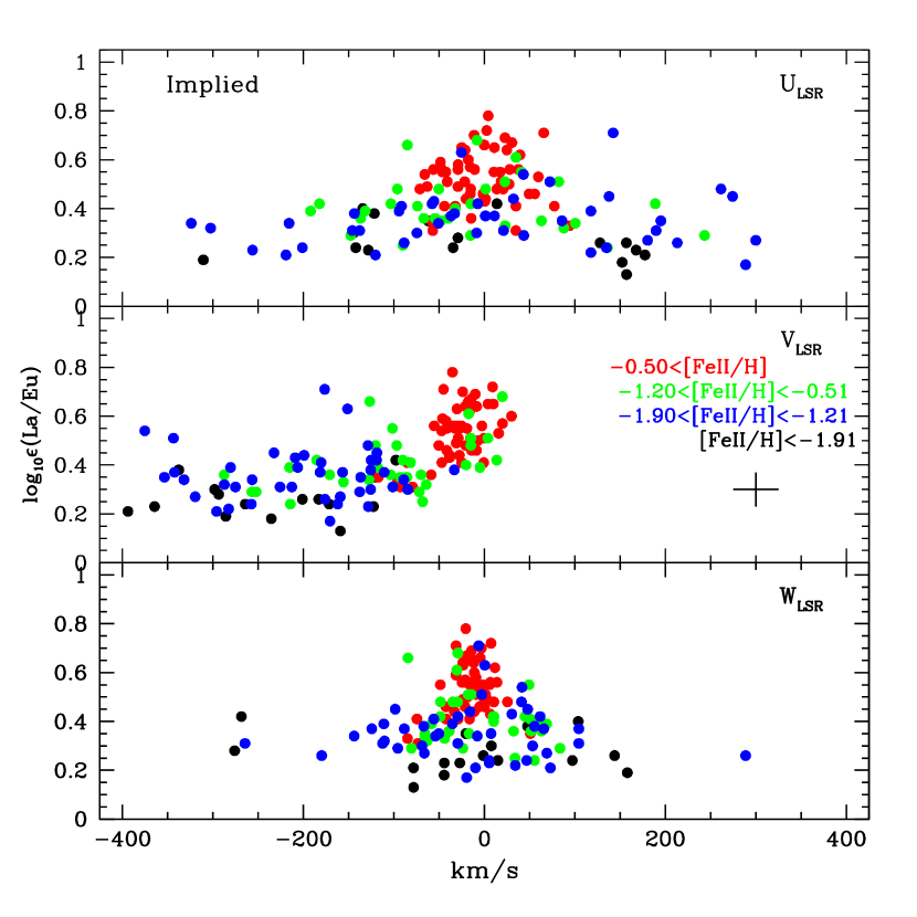
Figure 12: La/Eu as a function of space velocity components. Only stars with errors in U, V, and W less than 100 km/s are shown. These velocities are computed from distances that are in accord with the spectroscopically derived stellar parameters. The C-enhanced, $s$-process rich stars are not shown. The cross indicates a typical errorbar.

In Fig. 12 we plot La/Eu as functions of U, V, and W. We note a few features revealed in this figure. First, we find much stronger relationships with velocity than with metallicity, and the large scatter so evident in Fig. 7 has largely (but not totally) disappeared. With very few exceptions, low-velocity stars have a higher La/Eu ratio than high-velocity stars. This is especially evident in the U and W velocity distributions, where the stars with the highest $s$-process abundances group near 0 km/s, regardless of their overall iron content. In the V velocity distribution, although there is an overall increase in La/Eu with decreasing V (also largely independent of [Fe/H]), there still exists a low La/Eu group of stars with solar V motion and near-solar metallicities.

Secondly, in U and W, the velocity dispersion increases with decreasing $s$-process contributions, regardless of overall iron content. There are stars with only mild iron deficiencies ($-1.20<$[Fe/H]$<-0.51$) that have low U or W velocities and low La/Eu, but the range of U and W velocity values increases dramatically as La/Eu becomes smaller.

Thirdly, there is no metallicity bin that will only encompass the high La/Eu, low-velocity stars. In Fig. 12, lowering the boundary on the highest [Fe II/H] bin (say, to include all the stars in the low V velocity clump) introduces a significant tail of high-V, low-La/Eu stars in that metallicity bin. Many of the lower-metallicity stars in the low-V clump are not artifacts of the choice of metallicity bin.

Finally, the spread in La/Eu in the low V velocity “clump” stars is larger than the spread in La/Eu in the high V velocity “tail” stars ($\sim 0.4$ and $\sim 0.2$ dex, respectively). This may be coincidental, although the spread at low V is certainly real. From Edvardsson et al. (1993) we can get ages for most of the stars in the “clump”, and, as shown in Fig. 13 there is a distinct relationship between stellar age and La/Eu. This correlation is also present, although more muted, in [Fe II/H] and Eu II and La II, as shown in Fig. 14. Since the thick disk is characterized by high velocities and a $\sim$50 km/s rotation lag, it is more likely that these low-La, low-V stars are part of the old thin disk. Indeed, we can find no distinct contrast between thick disk and halo stars in log$\epsilon$(La/Eu), although several of our stars have been identified as such by other studies (see Fuhrmann 1998).

6 Conclusion

In this study we observed 159 giant and dwarf stars across a wide range of metallicity in order to measure the evolution of the abundance ratio La/Eu, a proxy for the $s$-/$r$-process ratio. We have found that the $s$-/$r$-process ratio does not increase monotonically with [Fe/H]. However, there is evidence for evolution in this ratio. At low metallicity, the abundances of La and Eu are approximately equal; near solar metallicity, La is consistently more abundant. The $s$-process contribution to individual stars varies widely even at near-solar metallicities. However, we find that on the average the dispersion in La and the dispersion in Eu individually are equal, indicating that the $r$-process contribution, while smaller overall, also varies.

Some of the variation in La/Eu can be attributed to the intrusion of different Galactic stellar populations. We find that when stars are separated by velocity, very little scatter in La/Eu remains. Rather, stars separate into high-velocity and low-velocity groups. The former group has essentially a single value of La/Eu (although there is some spread, and a few stars stand out in this respect; the overall spread in abundances is about 0.2 dex here). The latter group shows considerable dispersion still (about 0.4 dex overall), although at a higher overall La/Eu value. This variation is further reduced when stellar age is considered. The age correlation and the velocity data argue most strongly for evolution in the $s$-/$r$-ratio in the disk, with very little change throughout the halo. This sample also includes thick disk stars identified by other studies, although these are not readily distinguishable from the halo based solely on La/Eu.

Neither stellar population considerations nor measurement uncertainties can account for the persistently high La/Eu ratio at low metallicities, where the $r$-process is believed to be dominant. None of the stars studied here has a “pure $r$-process” value of La/Eu, in contrast to the $r$-process rich star BPS CS 22892-052, studied with the same La and Eu atomic data. It is still unclear whether this indicates that the $s$-process was indeed active in the halo at very low metallicities and established a “floor” in La/Eu for old stars or simply that the “pure $r$-process” value of La/Eu, despite extensive recent work, is in error.

Appendix A $s$- AND $r$-PROCESS SOLAR SYSTEM ABUNDANCES

The $s$- and $r$-neutron capture processes are responsible for the synthesis of almost all of the isotopes above iron - the exceptions being the relatively rare $p$-process nuclei. While a few of those isotopes are formed solely in one of those processes, most isotopes are a combination of the products of the $s$- and the $r$-process. The deconvolution of the solar system material into the individual isotopic contributions from the $s$-process and $r$-process has traditionally relied upon reproducing the (smooth behavior) of the “$\sigma$ N_s” curve (i.e., the product of the $n$-capture cross-section and $s$-process abundance). This so-called “classical” fit to the $s$-process is empirical and by definition model-independent. Extensive neutron capture cross section measurements (see Käppeler et al. 1989) thus allow the determination of the $s$-process abundance, N_s, contributions to each isotope. (Experimental determinations of individual $r$-process contributions are, in general, not experimentally possible at this time.) Subtracting these N_s values from the total solar abundances determines the residual isotopic $r$-process contributions, N_r, which are then summed to obtain solar elemental $r$- (and $s$-) process abundance distributions (see also the reviews by Cowan et al. 1991; Truran et al. 2002; Sneden & Cowan 2003 for further discussion).

Earlier tabulations of this solar deconvolution, based on this classical approach, were included in Sneden et al. (1996) and more recently in Burris et al. (2000). We have slightly revised and updated the Burris et al. values and list these elemental abundance distributions in Table 10. In particular the Nd values have been revised to incorporate more recent measurements from Wisshak et al. (1998). We note that these cross section experiments assumed total solar abundances from earlier compilations including Anders & Ebihara (1982) and Anders & Grevesse (1989). Thus the total abundances, based on a scale of Si = 10⁶ and listed in column (3), are approximately equal to, but slightly different than, the most recent solar abundance determinations from Lodders (2003). The elemental N_r and N_s values, listed in columns (4) and (6) respectively, are the summation of all of the isotopic contributions from these two processes. (In some cases due to small contributions from the $p$-process and uncertainties in the experimental cross sections and hence the $s$-process contributions, there are a few cases in which the sums of N_S and N_r are slightly different than the total abundances.) We also note that we have not included Zn (Z = 30) in this tabulation, in contrast to previous versions. This is due to Zn having a significant non-$n$-capture component from explosive charged-particle nucleosynthesis.

For each element we have also listed the fractional contribution of the $s$- and $r$-process. Thus it is seen that Eu is overwhelmingly (97%) synthesized by the $r$-process, while Ba is predominantly (85%) produced by the $s$-process in solar system material. In addition we have tabulated the abundances in spectroscopic units where log $\epsilon$(A) $\equiv$ log₁₀(N_A/N_H) + 12.0, for elements A and B. The spectroscopic units are then related to the abundance units by

$$Log\ \epsilon(El)=Log\ N(El)+1.54$$

(see Lodders 2003).

In addition to the classical approach for understanding the $s$-process, more sophisticated abundance predictions, based on $s$-process nucleosynthesis models in low-mass AGB stars, have also been developed (Arlandini et al., 1999). (The primary site for $s$-process nucleosynthesis is identified with low- or intermediate-mass stars, i.e., $M\simeq 0.8-8$ M_⊙; see Busso et al. 1999.) For comparison purposes we have tabulated the $s$- and $r$-process solar abundances determined for one particular set of predictions (i.e., the “stellar model”) from Arlandini et al. (1999). We have made one modification to those predictions by updating the La value on the basis of new neutron capture cross sections on ¹³⁹La (O’Brien et al., 2003).

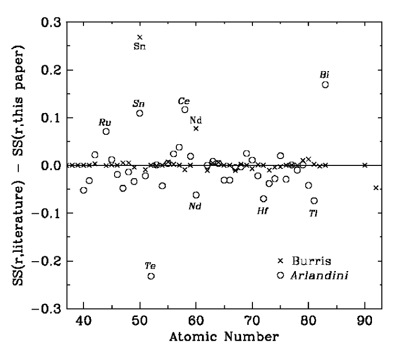
Figure 15: Comparison of the solar system $r$-process abundances re-evaluated in this paper (Table A) with previously-published values. For each atomic number, the ordinate value is the $r$-process abundance from the literature (X-symbols, Burris et al. 2000; open circles, Arlandini et al. 1999) minus the present value. Abundance discrepancies greater than 0.05 dex are labeled in the figure, and discussed in the Appendix.

A comparison of these latter abundance predictions with those obtained in the classical approach is shown in Figure 15. It is seen that in general there is a good overall agreement between the literature values for the $r$-process and both of the predictions. Nevertheless, there are some important differences: for example Te, Nd, and Bi. We also note a significant difference in the abundances determined from the classical approach and the stellar model calculations for the element Sn. Also, while not plotted there are also significant differences in the Y predictions. Interestingly, the abundance determined for this element from Arlandini et al. (1999) seems to give a much better fit to the observed $n$-capture abundances in some metal-poor halo stars (see e.g., Cowan et al. 2002a).

Table 1: Derived Stellar Parameters and Abundances

Star	note	$T_{\rm{eff}}$(K)	$T_{\rm{eff}}$(K)	$T_{\rm{eff}}$(K)	log $g$	log $g$	vt(km sec${}^{-}1$)	[Fe I/H]	# lines	[Fe II/H]	# lines	MV	d (pc)	log$\epsilon$(La/Eu)	[C/Fe]
		(Alonso)	(IRFM)	(Final)	(calc)
B+191185	1	$\cdots$	5328	5500	4.19	4.19	1.10	-1.09	14	-1.17	7	5.04	67	0.29	-0.25
B+521601		4911	4816	4911	2.10	2.10	2.05	-1.40	15	-1.34	7	0.13	541	0.38	-0.3
B-010306	1	$\cdots$	5680	5550	4.19	4.19	1.50	-1.13	10	-1.13	8	5.04	62	0.39	-0.15
B-012582		5148	5100	5148	2.86	2.86	1.20	-2.21	7	-2.09	7	1.78	364	0.98	0.8
G005-001	1	$\cdots$	5612	5500	4.32	4.32	0.80	-1.24	15	-1.28	7	5.26	91	0.29	-0.05
G009-036		5625	5265	5625	4.57	4.57	0.65	-1.17	10	-1.01	8	5.81	167	0.42	-0.25
G017-025	3	4966	4856	4966	4.26	4.26	0.80	-1.54	16	-1.44	9	5.88	48	0.54	-0.05
G023-014	1,2	$\cdots$	4529	5025	4.02	3.00	1.30	-1.64	15	-1.57	7	2.68*	312	0.25	-0.2
G028-043	2	5061	$\cdots$	5061	$\cdots$	4.50	0.80	-1.64	11	-1.55	3	6.39	48	0.31	-0.15
G029-025	1	$\cdots$	5115	5225	4.28	4.28	0.80	-1.09	14	-0.88	8	5.51	112	0.42	-0.05
G040-008	1,3	$\cdots$	5133	5200	4.08	4.08	0.50	-0.97	18	-0.88	9	5.03	83	0.32	-0.1
G058-025		6001	5996	6001	4.21	4.21	1.00	-1.40	8	-1.53	7	4.56	52	0.63	0.05
G059-001		$\cdots$	5299	5922	3.98	3.98	0.40	-0.95	16	-0.99	8	4.23	113	0.42	-0.15
G063-046	2	5705	5701	5705	3.69	4.25	1.30	-0.90	14	-0.89	8	4.94*	74	0.32	0
G068-003	1,2	$\cdots$	4787	4975	4.59	3.50	0.95	-0.76	19	-0.76	10	3.88*	104	0.33	0
G074-005		$\cdots$	5668	5668	4.24	4.24	1.50	-1.05	13	-1.23	8	4.96	57	0.34	0.05
G090-025		5441	5303	5303	4.46	4.46	1.20	-1.78	9	-1.79	4	5.98	28	0.45	-0.05
G095-57A		$\cdots$	4965	4965	4.40	4.40	0.90	-1.22	17	-1.15	6	6.15	24	0.66	-0.05
G095-57B	1,3	$\cdots$	4540	4800	4.57	4.57	0.60	-1.06	18	-0.95	5	6.78	24	0.46	-0.1
G102-020		5254	5223	5254	4.44	4.44	0.90	-1.25	15	-1.21	7	5.90	70	0.30	-0.2
G102-027	1,2	$\cdots$	5286	5600	2.88	3.75	1.05	-0.59	19	-0.53	12	3.80*	58	0.29	-0.05
G113-022	1,2	$\cdots$	5616	5525	$\cdots$	4.25	1.10	-1.18	14	-1.00	8	5.15*	75	0.55	-0.15
G122-051		$\cdots$	4864	4864	4.51	4.51	1.40	-1.43	15	-1.29	6	6.59	9	0.17	-0.05
G123-009	2	$\cdots$	5487	5487	$\cdots$	4.75	1.50	-1.25	14	-1.22	7	6.44*	63	0.42	-0.25
G126-036	2	$\cdots$	5487	5487	$\cdots$	4.50	0.60	-1.06	15	-0.92	9	5.75*	57	0.83	0.15
G126-062	3	5941	5998	5941	3.98	3.98	2.00	-1.59	5	-1.61	7	4.07	119	0.40	-0.05
G140-046		4980	4959	4980	4.42	4.42	0.70	-1.30	16	-1.34	4	6.25	59	0.95	-0.2
G153-021	1	$\cdots$	5190	5700	4.36	4.36	1.40	-0.70	14	-0.65	10	5.33	92	0.25	-0.2
G176-053		5593	5710	5593	4.50	4.50	1.20	-1.34	9	-1.39	7	5.72	66	0.24	-0.05
G179-022		$\cdots$	5082	5082	3.20	3.20	1.20	-1.35	15	-1.27	8	3.05	332	0.27	-0.25
G180-024		6059	5993	6059	4.09	4.09	0.50	-1.34	6	-1.30	8	4.22	125	0.39	-0.5
G188-022		$\cdots$	5827	5827	4.27	4.27	1.20	-1.52	7	-1.35	8	4.83	109	0.45	-0.35
G191-055	2	$\cdots$	5770	5770	$\cdots$	4.50	1.00	-1.63	7	-1.68	5	5.55*	78	0.48	-0.1
G192-043	2	6085	6101	6085	3.73	4.50	1.50	-1.50	7	-1.39	7	5.20*	97	0.23	0.07
G221-007		$\cdots$	5016	5016	3.37	3.37	0.90	-0.98	20	-0.90	10	3.56	115	0.39	0.05
HD002665		4990	5015	4990	2.34	2.34	2.00	-1.99	16	-2.04	9	0.66	236	0.23	-0.05
HD003008	1,2	4047	4141	4250	1.03	0.25	2.60	-2.08	18	-2.02	11	-3.49*	3868	0.30	-0.25
HD006755		$\cdots$	5105	5105	2.93	2.93	2.50	-1.68	14	-1.57	10	1.98	129	0.21	-0.2
HD006833	2	4402	4392	4402	$\cdots$	1.50	1.20	-0.85	12	-0.83	10	-0.65*	163	0.24	-0.2
HD008724		4535	4467	4535	1.40	1.40	1.40	-1.91	15	-1.69	10	-1.11	732	0.37	-0.25
HD021581		4870	4866	4870	2.27	2.27	1.40	-1.71	10	-1.68	7	0.61	390	0.39	-0.15
HD023798	1	$\cdots$	4294	4450	1.06	1.06	2.50	-2.26	7	-2.17	7	-1.81	1057	0.35	-0.55
HD025329		4842	4571	4842	4.66	4.66	0.60	-1.67	15	-1.56	2	7.18	18	$\cdots$	0.35
HD025532	2	5396	$\cdots$	5396	2.57	2.00	1.20	-1.34	15	-1.31	9	-0.64*	454	0.51	-0.25
HD026297		4322	4271	4322	1.11	1.11	1.80	-1.98	16	-1.76	9	-1.48	620	0.37	-0.45
HD029574	1	4020	3952	4250	0.80	0.80	2.20	-2.00	14	-1.80	8	-2.11	1165	0.26	-0.65
HD037828	1,2	$\cdots$	4299	4350	$\cdots$	1.50	1.85	-1.62	17	-1.42	9	-0.56*	282	0.41	-0.2
HD044007	2	4851	5007	4851	2.75	2.00	2.00	-1.72	16	-1.71	9	-0.04*	298	0.43	0
HD063791	1,2	$\cdots$	4556	4675	$\cdots$	2.00	2.00	-1.90	15	-1.67	10	0.19*	325	0.37	-0.25
HD074462	1,2	$\cdots$	4427	4700	$\cdots$	2.00	1.90	-1.52	7	-1.51	9	0.15*	471	0.22	-0.3
HD082590		6005	5945	6005	2.75	2.75	3.00	$\cdots$	0	-1.32	6	0.69	528	0.35	-1.05
HD085773	2	$\cdots$	4268	4268	0.87	0.50	2.00	-2.62	13	-2.39	7	-2.90*	2729	0.28	-0.45
HD101063	1	$\cdots$	4984	5150	3.25	3.25	1.70	-1.33	16	-1.27	7	2.74	210	0.21	-0.15
HD103036	1,2	$\cdots$	4103	4200	1.14	0.25	3.00	-2.04	12	-1.83	7	-3.39*	1990	0.47	-0.35
HD103545		4666	4528	4666	1.64	1.64	2.00	-2.45	10	-2.16	5	-0.68	1047	0.38	-0.4
HD105546		5190	5147	5190	2.49	2.49	1.60	-1.48	11	-1.41	6	0.79	365	0.42	-0.45
HD105755		$\cdots$	5701	5701	3.82	3.82	1.20	-0.83	17	-0.84	10	4.01	78	0.31	0
HD106516		$\cdots$	6166	6166	4.21	4.21	1.10	-0.81	13	-0.78	10	4.31	23	0.35	0
HD107752		$\cdots$	4649	4649	1.63	1.63	2	-2.78	8	-2.59	5	-0.68	1364	0.40	-0.55
HD108317		5234	5230	5234	2.68	2.68	2.00	-2.18	6	-2.28	7	1.26	221	0.23	-0.05
HD110184	2	4250	4185	4250	0.79	0.50	2.50	-2.72	11	-2.50	6	-2.87*	1662	0.24	-0.3
HD115444		4721	4661	4721	1.74	1.74	2.00	-2.90	8	-2.71	5	-0.49	784	0.26	-0.55
HD119516		$\cdots$	5382	5382	2.47	2.47	2.50	-2.11	7	-1.85	8	0.56	507	0.31	-1.15
HD121135		4934	4885	4934	1.91	1.91	1.60	-1.54	15	-1.37	8	-0.36	869	0.37	-0.45
HD122563		4572	4537	4572	1.36	1.36	2.90	-2.72	8	-2.61	7	-1.24	308	0.24	-0.6
HD122956		$\cdots$	4508	4508	1.55	1.55	1.60	-1.95	14	-1.69	10	-0.69	356	0.31	-0.3
HD124358		4688	4645	4688	1.57	1.57	2.10	-1.91	12	-1.64	7	-0.89	1128	0.26	-0.75
HD128279		5290	5316	5290	2.95	2.95	1.50	-2.01	8	-2.13	7	1.86	158	0.42	-0.1
HD132475		5788	5425	5425	3.56	3.56	2.30	-1.86	10	-1.68	6	3.61	92	0.54	-0.15
HD135148	2	$\cdots$	4183	4183	1.24	0.25	2.90	-2.17	12	-2.07	7	-3.36*	3333	0.19	0.8
HD141531		4461	4356	4356	1.14	1.14	2.20	-1.79	16	-1.62	9	-1.46	1292	0.27	-0.4
HD165195		4237	4316	4237	0.78	0.78	2.30	-2.60	13	-2.28	5	-2.14	646	0.18	-0.5
HD166161	1	4974	5179	5350	2.56	2.56	2.25	-1.23	16	-1.22	9	0.79	197	0.71	-0.1
HD171496		4485	4952	4952	2.37	2.37	1.40	-0.67	13	-0.64	6	0.75	246	0.40	-0.15
HD184266	1	5587	5565	6000	2.74	2.74	3.00	-1.43	7	-1.40	9	0.68	223	0.32	-0.55
HD186478		4598	4565	4598	1.43	1.43	2.00	-2.56	10	-2.44	7	-1.12	1025	0.21	-0.4
HD187111		4271	4276	4271	1.05	1.05	1.90	-1.97	11	-1.69	9	-1.54	615	0.31	-0.4
HD188510		5564	5373	5564	4.51	4.51	1.00	-1.32	14	-1.62	7	5.82	39	0.38	-0.1
HD193901		5750	5768	5750	4.46	4.46	1.50	-1.08	12	-1.16	8	5.43	44	0.29	-0.2
HD194598		$\cdots$	6044	6044	4.19	4.19	1.00	-1.08	15	-1.16	8	4.46	56	0.36	-0.05
HD201891		5909	5883	5909	4.19	4.19	1.00	-1.09	9	-1.10	7	4.59	35	0.34	0.05
HD204543		4672	4600	4672	1.49	1.49	2.00	-1.87	16	-1.72	9	-1.09	725	0.44	-0.55
HD206739		4647	4548	4647	1.78	1.78	1.90	-1.72	16	-1.61	9	-0.33	574	0.30	-0.2
HD210295	1,2	$\cdots$	4574	4750	$\cdots$	2.50	1.55	-1.46	19	-1.25	9	1.33*	441	0.24	-0.2
HD214362		5727	5780	5727	2.62	2.62	2.00	-1.87	4	-1.69	9	0.62	493	0.34	-1.05
HD218857		$\cdots$	5103	5103	2.44	2.44	1.90	-1.90	10	-2.01	8	0.81	410	0.26	-0.05
HD221170		4410	4402	4410	1.09	1.09	1.70	-2.35	12	-2.03	8	-1.67	689	0.13	-0.5
HD232078	1,2	3654	3628	3875	0.93	0.50	2.10	-1.69	11	-1.40	8	-1.89*	120	0.34	-0.15
HD233666	2	$\cdots$	5157	5157	$\cdots$	2.00	1.70	-1.79	9	-1.81	8	-0.39*	867	0.35	-0.35

Note. — In Column 2, a (1) indicates a star for which $T_{\rm{eff}}$was adopted based solely on Fe Ews, a (2) indicates a star for which log$~{}g$ was set by forcing agreement between [Fe I/H] and [Fe II/H], and a (3) indicates a star identified as a spectrscopic binary by Latham et al. (2002). A * marks M_V derived from an adopted $T_{\rm{eff}}$and log$~{}g$.

Table 2: Line Parameters

wavelength(Å)	Excitation Potential (EV)	log$gf$
Fe I
4445.48	0.087	-5.44
5225.53	0.110	-4.79
5247.06	0.087	-4.95
5250.22	0.121	-4.94
5326.15	3.570	-2.07
5412.79	4.440	-1.72
5491.84	4.190	-2.29
5600.23	4.260	-1.42
5855.08	4.610	-1.48
6120.26	0.910	-5.97
6151.62	2.176	-3.30
6481.88	2.279	-2.98
6498.95	0.958	-4.70
6518.37	2.830	-2.45
6609.12	2.559	-2.69
6625.03	1.010	-5.34
6739.52	1.560	-4.79
6750.16	2.424	-2.62
6752.71	4.640	-1.20
7189.16	3.070	-2.77
7723.21	2.280	-3.62
Fe II
4620.52	2.828	-3.19
4656.98	2.891	-3.57
5234.63	3.221	-2.22
5264.79	3.250	-3.23
5414.08	3.221	-3.48
5525.13	3.267	-3.94
6432.68	2.891	-3.51
6516.08	2.891	-3.38
7224.46	3.890	-3.28
7515.84	3.903	-3.37
7711.73	3.903	-2.45
La II
3988.52	0.400	0.21
3995.75	0.170	-0.06
4086.71	0.000	-0.07
4123.22	0.320	0.13
4333.75	0.170	-0.06
4662.50	0.000	-1.24
5122.99	0.320	-0.85
5303.53	0.320	-1.35
5797.57	0.240	-1.36
6390.48	0.320	-1.41
Eu II
3819.67	0.000	0.51
3907.11	0.207	0.17
4129.72	0.000	0.22
4205.04	0.000	0.21
6437.64	1.319	-0.32
6645.06	1.379	0.12
7217.56	1.229	-0.35

Table 3: La Abundances

Star	3988 Å	3995 Å	4086 Å	4123 Å	4333 Å	4662 Å	5122 Å	5303 Å	5797 Å	6930 Å	log$\epsilon$(Laavg)	$\sigma$
BD +191185	0	0.13	0.08	0.08	0.03	$\cdots$	$\cdots$	$\cdots$	$\cdots$	$\cdots$	0.06	0.05
BD +511696	-0.08	-0.03	-0.1	-0.01	$\cdots$	$\cdots$	$\cdots$	$\cdots$	$\cdots$	$\cdots$	-0.06	0.04
BD +521601	-0.19	-0.14	-0.24	-0.19	-0.14	-0.12	-0.09	-0.09	-0.04	-0.06	-0.13	0.06
BD -010306	0.13	0.11	0.09	0.16	0.16	0.06	$\cdots$	$\cdots$	$\cdots$	$\cdots$	0.12	0.04
BD -012582	-0.09	-0.12	-0.04	-0.19	$\cdots$	0.04	0.01	$\cdots$	$\cdots$	$\cdots$	-0.05	0.08
G005-001	-0.13	-0.15	-0.01	-0.03	-0.13	$\cdots$	$\cdots$	$\cdots$	$\cdots$	$\cdots$	-0.09	0.06
G009-036	$\cdots$	0.29	0.39	0.12	0.22	$\cdots$	$\cdots$	$\cdots$	$\cdots$	$\cdots$	0.26	0.11
G023-014	-0.36	-0.32	-0.37	-0.3	-0.33	-0.35	-0.25	$\cdots$	$\cdots$	$\cdots$	-0.33	0.04
G028-043	$\cdots$	-0.17	-0.27	$\cdots$	-0.22	$\cdots$	$\cdots$	$\cdots$	$\cdots$	$\cdots$	-0.22	0.05
G029-025	$\cdots$	0.18	0.21	0.26	0.11	$\cdots$	$\cdots$	$\cdots$	$\cdots$	$\cdots$	0.19	0.06
G058-025	0.01	-0.04	-0.04	0.03	$\cdots$	$\cdots$	$\cdots$	$\cdots$	$\cdots$	$\cdots$	-0.03	0.03
G059-001	$\cdots$	0.09	0.11	0.21	0.06	0.16	$\cdots$	$\cdots$	$\cdots$	$\cdots$	0.13	0.06
G063-046	0.22	0.27	0.22	0.32	0.32	$\cdots$	$\cdots$	$\cdots$	$\cdots$	$\cdots$	0.27	0.05
G068-003	0.44	0.43	0.61	0.61	0.36	0.51	$\cdots$	$\cdots$	$\cdots$	0.46	0.49	0.09
G074-005	0.1	0.07	0.1	0.12	0.17	$\cdots$	$\cdots$	$\cdots$	$\cdots$	$\cdots$	0.11	0.04
G090-025	-0.56	-0.46	$\cdots$	-0.51	$\cdots$	$\cdots$	$\cdots$	$\cdots$	$\cdots$	$\cdots$	-0.51	0.05
G095-57A	0.37	0.38	0.39	0.39	0.37	0.47	$\cdots$	0.62	$\cdots$	$\cdots$	0.43	0.09
G102-020	-0.02	0.08	0.03	0.03	-0.22	$\cdots$	$\cdots$	$\cdots$	$\cdots$	$\cdots$	-0.02	0.12
G102-027	0.7	0.67	0.77	0.65	0.62	0.7	0.7	$\cdots$	$\cdots$	$\cdots$	0.69	0.05
G113-022	0.41	0.34	0.47	0.36	0.44	0.48	0.46	$\cdots$	$\cdots$	$\cdots$	0.42	0.05
G122-051	-0.17	-0.07	-0.07	-0.07	-0.1	$\cdots$	$\cdots$	$\cdots$	$\cdots$	$\cdots$	-0.1	0.04
G123-009	0.23	0.18	0.28	0.16	0.18	$\cdots$	$\cdots$	$\cdots$	$\cdots$	$\cdots$	0.21	0.05
G126-036	0.86	0.91	0.81	0.81	0.84	0.96	0.94	$\cdots$	$\cdots$	0.81	0.87	0.06
G140-046	0.53	0.47	0.45	0.50	0.7	0.55	0.4	0.7	$\cdots$	$\cdots$	0.54	0.11
G153-021	0.61	0.57	0.56	0.64	0.54	0.64	$\cdots$	$\cdots$	$\cdots$	$\cdots$	0.59	0.04
G176-053	-0.02	-0.1	-0.08	-0.1	$\cdots$	$\cdots$	$\cdots$	$\cdots$	$\cdots$	$\cdots$	-0.08	0.04
G179-022	0	0.02	-0.03	-0.05	-0.02	0.1	0.1	$\cdots$	$\cdots$	$\cdots$	0.02	0.06
G180-024	0	-0.3	-0.25	-0.2	-0.2	$\cdots$	$\cdots$	$\cdots$	$\cdots$	$\cdots$	-0.19	0.11
G188-022	$\cdots$	$\cdots$	-0.18	-0.08	-0.11	$\cdots$	$\cdots$	$\cdots$	$\cdots$	$\cdots$	-0.12	0.05
G191-055	-0.28	$\cdots$	-0.48	-0.48	$\cdots$	$\cdots$	$\cdots$	$\cdots$	$\cdots$	$\cdots$	-0.41	0.12
G192-043	0.07	-0.03	0.02	-0.13	$\cdots$	$\cdots$	$\cdots$	$\cdots$	$\cdots$	$\cdots$	-0.02	0.09
G221-007	0.24	0.27	0.42	0.14	0.22	0.24	0.32	$\cdots$	$\cdots$	0.37	0.28	0.09
HD002665	-0.99	-0.94	-1.02	-0.89	-0.84	-0.89	-0.84	$\cdots$	$\cdots$	$\cdots$	-0.92	0.07
HD003008	-0.84	-0.64	-0.74	-0.89	$\cdots$	-0.77	-0.79	-0.84	$\cdots$	-0.84	-0.79	0.08
HD006755	-0.28	-0.34	-0.38	-0.46	-0.26	-0.14	-0.16	$\cdots$	$\cdots$	$\cdots$	-0.29	0.12
HD006833	0.11	0.23	0.48	0.28	0.23	0.38	0.45	0.41	$\cdots$	0.45	0.34	0.13
HD008724	-0.5	-0.47	-0.45	-0.47	-0.47	-0.51	-0.55	-0.5	$\cdots$	-0.5	-0.49	0.03
HD021581	-0.48	-0.43	-0.37	-0.38	-0.51	-0.28	-0.38	-0.43	-0.41	-0.53	-0.42	0.07
HD023798	-1	-1	-1.15	-1.15	-1.1	-1	-1	-0.77	$\cdots$	-0.95	-1.01	0.12
HD025329	$\cdots$	-0.09	-0.01	-0.04							-0.05	0.04
HD025532	-0.11	-0.16	-0.06	-0.16	-0.13	-0.11	-0.08	-0.11	$\cdots$	-0.21	-0.13	0.05
HD026297	-0.93	-0.81	-0.93	-0.88	-0.88	-0.83	-0.83	-0.83	-0.76	-0.81	-0.85	0.05
HD029574	-0.51	-0.31	-0.26	-0.46	-0.34	-0.36	-0.39	-0.38	$\cdots$	-0.31	-0.37	0.08
HD037828	-0.13	-0.06	-0.18	-0.16	-0.18	-0.13	$\cdots$	-0.06	$\cdots$	-0.02	-0.12	0.06
HD044007	-0.51	-0.53	-0.57	-0.55	-0.53	-0.51	-0.5	-0.45	$\cdots$	-0.4	-0.51	0.05
HD063791	-0.54	-0.58	-0.69	-0.62	-0.56	-0.47	$\cdots$	-0.39	$\cdots$	$\cdots$	-0.55	0.1
HD074462	-0.26	-0.16	-0.24	-0.24	-0.19	-0.1	-0.12	-0.09	$\cdots$	-0.09	-0.17	0.07
HD082590	-0.1	-0.1	-0.1	-0.15	-0.12	$\cdots$	$\cdots$	$\cdots$	$\cdots$	$\cdots$	-0.11	0.02
HD085773	-1.47	-1.59	-1.65	-1.52	-1.67	-1.43	$\cdots$	$\cdots$	$\cdots$	$\cdots$	-1.56	0.1
HD101063	0.26	0.26	0.11	0.11	0.23	0.28	$\cdots$	$\cdots$	$\cdots$	$\cdots$	0.21	0.08
HD103036	-0.59	-0.49	-0.54	-0.57	-0.72	-0.61	$\cdots$	-0.71	$\cdots$	-0.74	-0.62	0.09
HD103545	-1.2	-1.16	-1.2	-1.2	-1.16	$\cdots$	$\cdots$	$\cdots$	$\cdots$	$\cdots$	-1.18	0.02
HD105546	-0.17	-0.17	-0.11	-0.29	-0.16	-0.1	-0.14	-0.01	0.01	$\cdots$	-0.13	0.09
HD105755	0.32	0.32	0.34	0.39	0.29	$\cdots$	$\cdots$	$\cdots$	$\cdots$	$\cdots$	0.33	0.04
HD106516	0.32	0.27	0.42	0.32	0.22	$\cdots$	$\cdots$	$\cdots$	$\cdots$	$\cdots$	0.31	0.07
HD107752	$\cdots$	$\cdots$	-1.54	-1.64	$\cdots$	$\cdots$	$\cdots$	$\cdots$	$\cdots$	$\cdots$	-1.59	0.07
HD108317	-1.01	-1.01	-1.06	-1.01	$\cdots$	$\cdots$	$\cdots$	$\cdots$	$\cdots$	$\cdots$	-1.02	0.03
HD110184	-1.49	-1.42	-1.49	-1.47	-1.47	$\cdots$	-1.47	$\cdots$	$\cdots$	$\cdots$	-1.47	0.03
HD115444	-1.31	-1.31	-1.29	-1.46	-1.36	$\cdots$	$\cdots$	$\cdots$	$\cdots$	$\cdots$	-1.35	0.07
HD119516	-0.55	-0.55	-0.62	-0.65	-0.6	$\cdots$	$\cdots$	$\cdots$	$\cdots$	$\cdots$	-0.59	0.04
HD121135	-0.39	-0.41	-0.31	-0.36	-0.36	-0.31	$\cdots$	-0.31	$\cdots$	-0.21	-0.33	0.06
HD122563	$\cdots$	-2.25	-2.45	-2.35	$\cdots$	$\cdots$	$\cdots$	$\cdots$	$\cdots$	$\cdots$	-2.35	0.1
HD122956	-0.52	-0.49	-0.49	-0.62	-0.52	-0.39	-0.42	-0.4	$\cdots$	$\cdots$	-0.48	0.08
HD124358	-0.65	-0.7	-0.8	-0.72	-0.75	-0.6	-0.65	-0.57	$\cdots$	$\cdots$	-0.68	0.08
HD128279	$\cdots$	-1.35	-1.05	-1.05	-1.25	$\cdots$	$\cdots$	$\cdots$	$\cdots$	$\cdots$	-1.18	0.15
HD132475	-0.37	-0.37	-0.35	-0.4	-0.4	$\cdots$	$\cdots$	$\cdots$	$\cdots$	$\cdots$	-0.38	0.02
HD135148	-0.66	-0.66	-0.91	-0.91	-0.68	-0.76	$\cdots$	-0.81	$\cdots$	-0.71	-0.76	0.1
HD141531	$\cdots$	-0.42	-0.53	-0.51	-0.44	$\cdots$	-0.46	-0.42	-0.41	-0.41	-0.45	0.05
HD165195	-1.18	-1.14	-1.24	-1.22	-1.14	-1.09	-1.19	-1.14	$\cdots$	-1.14	-1.16	0.05
HD166161	0.23	0.24	0.14	0.14	0.19	$\cdots$	0.32	0.24	0.29	0.29	0.23	0.06
HD171496	0.4	0.5	0.6	0.33	0.52	0.54	0.6	0.6	$\cdots$	0.53	0.51	0.09
HD184266	-0.14	-0.14	-0.04	-0.14	-0.09	$\cdots$	$\cdots$	$\cdots$	$\cdots$	$\cdots$	-0.11	0.04
HD186478	-1.29	-1.24	-1.26	-1.46	-1.29	$\cdots$	-1.19	$\cdots$	$\cdots$	$\cdots$	-1.29	0.09
HD187111	-0.57	-0.52	-0.72	-0.56	-0.62	-0.5	-0.57	-0.47	-0.57	-0.57	-0.57	0.07
HD188510	$\cdots$	-0.1	-0.2	-0.13	$\cdots$	$\cdots$	$\cdots$	$\cdots$	$\cdots$	$\cdots$	-0.14	0.05
HD193901	0.16	0.06	0.26	0.24	0.21	$\cdots$	$\cdots$	$\cdots$	$\cdots$	$\cdots$	0.19	0.08
HD194598	0.04	0.06	0.11	0.11	0.08	$\cdots$	$\cdots$	$\cdots$	$\cdots$	$\cdots$	0.08	0.03
HD201891	0.02	0.09	0.17	0.22	0.09	$\cdots$	$\cdots$	$\cdots$	$\cdots$	$\cdots$	0.12	0.08
HD204543	-0.51	-0.55	-0.6	-0.63	-0.6	-0.5	-0.51	-0.46	-0.62	-0.45	-0.54	0.07
HD206739	-0.41	-0.3	-0.46	-0.41	-0.36	-0.26	-0.23	-0.23	$\cdots$	-0.26	-0.32	0.09
HD210295	-0.17	-0.15	-0.2	-0.2	-0.04	0.03	$\cdots$	0.05	$\cdots$	$\cdots$	-0.1	0.11
HD214362	-0.43	-0.48	-0.53	-0.53	-0.45	$\cdots$	$\cdots$	$\cdots$	$\cdots$	$\cdots$	-0.48	0.05
HD218857	-1.13	-1.18	-1.06	-1.18	-1.23	$\cdots$	$\cdots$	$\cdots$	$\cdots$	$\cdots$	-1.16	0.06
HD221170	-0.74	-0.7	-0.7	-0.8	-0.7	-0.64	-0.72	-0.72	$\cdots$	-0.73	-0.72	0.04
HD232078	$\cdots$	$\cdots$	$\cdots$	-0.32	-0.45	-0.4	$\cdots$	-0.38	$\cdots$	-0.33	-0.38	0.05
HD233666	-0.74	-0.7	-0.67	-0.67	-0.68	-0.62	$\cdots$	$\cdots$	$\cdots$	$\cdots$	-0.68	0.04

Table 4: Eu Abundances

Star	3918 Å	3907 Å	4129 Å	4205 Å	6437 Å	6645 Å	7217 Å	log$\epsilon$(Euavg)	$\sigma$
BD +191185	$\cdots$	$\cdots$	-0.23	-0.23	$\cdots$	$\cdots$	$\cdots$	-0.23	0
BD +511696	-0.36	$\cdots$	-0.39	-0.37	$\cdots$	$\cdots$	$\cdots$	-0.37	0.02
BD +521601	$\cdots$	-0.6	-0.55	-0.5	$\cdots$	-0.4	$\cdots$	-0.51	0.09
BD -010306	$\cdots$	-0.35	-0.25	-0.2	$\cdots$	$\cdots$	$\cdots$	-0.27	0.08
BD -012582	-1.05	-1.07	-1.03	-0.98	$\cdots$	$\cdots$	$\cdots$	-1.03	0.04
G005-001	$\cdots$	-0.34	-0.41	-0.39	$\cdots$	$\cdots$	$\cdots$	-0.38	0.04
G009-036	$\cdots$	-0.09	-0.22	-0.17	$\cdots$	$\cdots$	$\cdots$	-0.16	0.07
G023-014	$\cdots$	-0.64	-0.68	-0.59	$\cdots$	-0.41	$\cdots$	-0.58	0.12
G028-043	$\cdots$	$\cdots$	-0.58	-0.48	$\cdots$	$\cdots$	$\cdots$	-0.53	0.07
G029-025	$\cdots$	$\cdots$	-0.25	-0.2	$\cdots$	$\cdots$	$\cdots$	-0.23	0.04
G058-025	$\cdots$	-0.65	-0.75	-0.58	$\cdots$	$\cdots$	$\cdots$	-0.66	0.09
G059-001	$\cdots$	$\cdots$	-0.35	-0.22	$\cdots$	$\cdots$	$\cdots$	-0.29	0.09
G063-046	$\cdots$	-0.02	-0.09	-0.04	$\cdots$	$\cdots$	$\cdots$	-0.05	0.04
G068-003	$\cdots$	$\cdots$	0.15	0.16	$\cdots$	0.18	$\cdots$	0.16	0.02
G074-005	$\cdots$	-0.26	-0.26	-0.19	$\cdots$	$\cdots$	$\cdots$	-0.23	0.06
G090-025	$\cdots$	$\cdots$	$\cdots$	-0.97	$\cdots$	$\cdots$	$\cdots$	-0.97	$\cdots$
G095-57A	$\cdots$	-0.34	$\cdots$	-0.16	$\cdots$	-0.19	$\cdots$	-0.23	0.1
G102-020	$\cdots$	$\cdots$	-0.36	-0.28	$\cdots$	$\cdots$	$\cdots$	-0.32	0.06
G102-027	$\cdots$	0.37	0.31	0.41	$\cdots$	0.49	$\cdots$	0.4	0.08
G113-022	$\cdots$	$\cdots$	-0.12	-0.13	$\cdots$	$\cdots$	$\cdots$	-0.13	0.01
G122-051	$\cdots$	$\cdots$	-0.25	-0.28	$\cdots$	$\cdots$	$\cdots$	-0.27	0.02
G123-009	$\cdots$	$\cdots$	-0.18	-0.23	$\cdots$	$\cdots$	$\cdots$	-0.21	0.04
G126-036	$\cdots$	0.03	0.03	0.05	$\cdots$	$\cdots$	$\cdots$	0.04	0.01
G140-046	$\cdots$	$\cdots$	-0.44	-0.38	$\cdots$	$\cdots$	$\cdots$	-0.41	0.04
G153-021	$\cdots$	0.33	0.33	0.33	$\cdots$	0.36	$\cdots$	0.34	0.01
G176-053	$\cdots$	-0.31	-0.36	-0.29	$\cdots$	$\cdots$	$\cdots$	-0.32	0.04
G179-022	$\cdots$	-0.26	-0.28	-0.22	$\cdots$	-0.11	$\cdots$	-0.22	0.08
G180-024	$\cdots$	-0.61	-0.51	-0.61	$\cdots$	$\cdots$	$\cdots$	-0.58	0.06
G188-022	-0.72	-0.52	-0.52	-0.62	$\cdots$	$\cdots$	$\cdots$	-0.6	0.1
G191-055	$\cdots$	$\cdots$	$\cdots$	-0.89	$\cdots$	$\cdots$	$\cdots$	-0.89	$\cdots$
G192-043	-0.27	$\cdots$	-0.24	-0.24	$\cdots$	$\cdots$	$\cdots$	-0.25	0.02
G221-007	$\cdots$	-0.11	-0.14	-0.07	$\cdots$	$\cdots$	$\cdots$	-0.11	0.04
HD002665	$\cdots$	-1.16	-1.15	-1.13	$\cdots$	$\cdots$	$\cdots$	-1.15	0.02
HD003008	$\cdots$	-1.35	-0.92	-1	$\cdots$	-1.08	$\cdots$	-1.09	0.19
HD006755	$\cdots$	-0.53	-0.54	-0.52	$\cdots$	-0.42	$\cdots$	-0.5	0.06
HD006833	$\cdots$	$\cdots$	$\cdots$	$\cdots$	0.13	0.14	0.04	0.1	0.06
HD008724	$\cdots$	-0.9	-0.86	-0.86	-0.88	-0.81	$\cdots$	-0.86	0.03
HD021581	$\cdots$	-0.86	-0.79	-0.79	$\cdots$	-0.81	$\cdots$	-0.81	0.03
HD023798	$\cdots$	$\cdots$	-1.41	-1.36	$\cdots$	-1.31	$\cdots$	-1.36	0.05
HD025329
HD025532	-0.71	-0.64	-0.65	-0.59	$\cdots$	-0.62	$\cdots$	-0.64	0.05
HD026297	$\cdots$	-1.29	-1.19	-1.21	$\cdots$	-1.19	$\cdots$	-1.22	0.05
HD029574	$\cdots$	$\cdots$	-0.64	-0.67	$\cdots$	-0.59	$\cdots$	-0.63	0.04
HD037828	$\cdots$	$\cdots$	-0.54	-0.59	$\cdots$	-0.51	-0.49	-0.53	0.04
HD044007	-1.08	-0.96	-0.94	-0.9	$\cdots$	-0.81	$\cdots$	-0.94	0.1
HD063791	$\cdots$	-0.99	-0.93	-0.9	$\cdots$	-0.85	$\cdots$	-0.92	0.06
HD074462	$\cdots$	-0.5	-0.4	-0.4	-0.3	-0.35	$\cdots$	-0.39	0.07
HD082590	-0.54	-0.41	-0.44	-0.44	$\cdots$	$\cdots$ -	$\cdots$	-0.46	0.06
HD085773	$\cdots$	-1.86	-1.83	-1.83	$\cdots$	$\cdots$	$\cdots$	-1.84	0.02
HD101063	$\cdots$	-0.05	-0.05	0.05	$\cdots$	0.1	-0.03	0	0.07
HD103036	$\cdots$	-0.95	-1.15	-1.15	$\cdots$	-1.1	$\cdots$	-1.09	0.09
HD103545	$\cdots$	-1.64	-1.55	-1.54	$\cdots$	-1.5	$\cdots$	-1.56	0.06
HD105546	$\cdots$	-0.53	-0.6	-0.54	$\cdots$	$\cdots$	$\cdots$	-0.56	0.04
HD105755	$\cdots$	$\cdots$	-0.03	0.01	$\cdots$	0.08	$\cdots$	0.02	0.06
HD106516	$\cdots$	-0.11	-0.04	0.04	$\cdots$	$\cdots$	$\cdots$	-0.04	0.08
HD107752	$\cdots$	$\cdots$	-1.9	-2.07	$\cdots$	$\cdots$	$\cdots$	-1.99	0.12
HD108317	-1.32	-1.22	-1.24	-1.22	$\cdots$	$\cdots$	$\cdots$	-1.25	0.05
HD110184	-1.83	-1.61	-1.68	-1.65	$\cdots$	-1.78	$\cdots$	-1.71	0.09
HD115444	-1.65	-1.57	-1.62	-1.61	$\cdots$	$\cdots$	$\cdots$	-1.61	0.03
HD119516	-0.96	-0.86	$\cdots$	-0.89	$\cdots$	$\cdots$	$\cdots$	-0.9	0.05
HD121135	$\cdots$	-0.77	-0.7	-0.7	$\cdots$	-0.62	$\cdots$	-0.7	0.06
HD122563	$\cdots$	$\cdots$	-2.56	-2.61	$\cdots$	$\cdots$	$\cdots$	-2.59	0.04
HD122956	$\cdots$	-0.86	-0.83	-0.8	$\cdots$	-0.68	$\cdots$	-0.79	0.08
HD124358	$\cdots$	-0.96	-0.96	-0.96	$\cdots$	-0.87	$\cdots$	-0.94	0.04
HD128279	-1.63	$\cdots$	-1.51	-1.56	$\cdots$	$\cdots$	$\cdots$	-1.57	0.06
HD132475	-0.93	$\cdots$	-0.98	-0.85	$\cdots$	$\cdots$	$\cdots$	-0.92	0.07
HD135148	$\cdots$	-0.95	-0.92	-0.87	$\cdots$	-1.05	$\cdots$	-0.95	0.08
HD141531	$\cdots$	$\cdots$	-0.65	-0.74	$\cdots$	-0.77	-0.72	-0.72	0.05
HD165195	-1.37	-1.27	-1.35	-1.33	$\cdots$	-1.4	$\cdots$	-1.34	0.05
HD166161	$\cdots$	-0.52	-0.52	-0.47	$\cdots$	-0.42	$\cdots$	-0.48	0.05
HD171496	$\cdots$	$\cdots$	0.1	0.04	0.14	0.14	$\cdots$	0.11	0.05
HD184266	-0.47	-0.5	-0.4	-0.35	$\cdots$	$\cdots$	$\cdots$	-0.43	0.07
HD186478	-1.55	-1.53	-1.45	-1.45	$\cdots$	$\cdots$	$\cdots$	-1.5	0.05
HD187111	$\cdots$	-0.93	-0.88	-0.9	-0.88	-0.8	$\cdots$	-0.88	0.05
HD188510	$\cdots$	-0.41	-0.54	-0.61	$\cdots$	$\cdots$	$\cdots$	-0.52	0.1
HD193901	$\cdots$	-0.05	-0.15	-0.1	$\cdots$	$\cdots$	$\cdots$	-0.1	0.05
HD194598	$\cdots$	-0.33	-0.27	-0.25	$\cdots$	$\cdots$	$\cdots$	-0.28	0.04
HD201891	$\cdots$	-0.29	-0.19	-0.19	$\cdots$	$\cdots$	$\cdots$	-0.22	0.06
HD204543	$\cdots$	-1.01	-0.98	-0.96	$\cdots$	$\cdots$	$\cdots$	-0.98	0.03
HD206739	$\cdots$	-0.72	-0.64	-0.58	$\cdots$	-0.55	$\cdots$	-0.62	0.07
HD210295	$\cdots$	$\cdots$	-0.38	-0.45	-0.28	-0.25	$\cdots$	-0.34	0.09
HD214362	$\cdots$	-0.89	-0.79	-0.77	$\cdots$	$\cdots$	$\cdots$	-0.82	0.06
HD218857	-1.44	-1.29	-1.44	-1.49	$\cdots$	$\cdots$	$\cdots$	-1.42	0.09
HD221170	$\cdots$	-0.88	-0.89	-0.86	-0.66	-0.89	-0.91	-0.85	0.09
HD232078	$\cdots$	$\cdots$	$\cdots$	-0.86	-0.56	-0.66	-0.81	-0.72	0.14

Table 5: Kinematics

Star	ULSR	error	VLSR	error	WLSR	error
	km/s	km/s	km/s	km/s	km/s	km/s
BD +191185	234.3	9.3	-240.3	45.8	90.5	14.3
BD +521601	-42.1	9.9	-21.3	2.5	-60	3.9
BD -010306	-201.1	31.9	-203.2	34.4	65.2	13.7
BD -012582	66	11.2	-163.7	27.4	-106.7	18
G 005-001	34.5	2.9	-125.8	19.7	-88.7	16.8
G 009-036	179.8	24.1	-173.3	31.4	52	13.9
G 017-025	-88.3	10.1	-172.1	23.6	-137.1	9.6
G 023-014	$\cdots$	$\cdots$	$\cdots$	$\cdots$	$\cdots$	$\cdots$
G 028-043	180.7	78.1	-263.1	84.4	-22.4	49.9
G 029-025	-112.4	19	-108.6	7.8	17.5	7.5
G 040-008	57.8	3.6	-131.1	23.8	-64.3	7.5
G 058-025	-34.5	2.2	-139.3	20.1	7.4	8.1
G 059-001	-191.3	32.1	-78.1	13.3	-41.8	7.3
G 063-046	78.8	30.8	-52.3	19.5	-56.3	11.7
G 068-003	13.9	3.7	-143.8	24.9	-37.1	34.1
G 074-005	-59.8	7.3	-77.1	15	-47.1	5.9
G 090-025	265.2	9.8	-220.5	43.1	-91.6	3.1
G 095-57A	-94.2	8.5	-114.7	22.6	-77.4	11.4
G 095-57B	-95.7	8.5	-116.2	22.9	-80	11.8
G 102-020	-17.6	0.9	-72.7	11.2	60.2	10.7
G 102-027	-24.4	4.6	-59.9	18.6	-16.8	4.3
G 113-022	32	25	-89.6	19.8	56.2	14
G 122-051	279.6	42.1	-158.6	25.5	-12.6	13.6
G 123-009	-66.8	33	-107.2	40	-22.4	4.9
G 126-036	85.4	32.2	-89	1.7	-29	19.7
G 126-062	-303.4	41.9	-276.9	5.3	5.2	23.8
G 140-046	114.4	19.2	-192.6	31.9	41.7	7
G 153-021	-99.1	7.6	-56.2	8.8	40.8	12.7
G 176-053	-210.1	31.1	-245.6	43.7	53.6	0.7
G 179-022	290.9	43.3	-147.3	31.1	75.9	1.6
G 180-024	108.7	25	-268.5	29	-28.4	15.4
G 188-022	128.7	24.2	-106.8	3.1	54.7	4
G 191-055	252.4	1.4	-116.7	30.6	48	35
G 192-043	-265.2	37.2	-116.3	65.3	12.3	21.3
G 221-007	-140.8	22.7	-105.9	19	-51.5	9
HD 002665	158.6	5.1	-352.5	4.7	-37.3	12.6
HD 003008	-153.6	61	-286.1	93.5	14.6	22.5
HD 006755	-129.4	52.1	-478.4	36.2	79.9	12.1
HD 006833	127	5.7	-202.5	4.4	62.3	10
HD 008724	2.2	9.2	-330.4	46.2	-81.6	26.8
HD 018768	$\cdots$	$\cdots$	$\cdots$	$\cdots$	$\cdots$	$\cdots$
HD 021581	-103.4	2.3	-194.3	31.7	-104.2	1.9
HD 022879	-105.2	1.5	-84.9	1.5	-41.4	1.6
HD 023798	-71.1	6.8	-108.3	11.6	-13.6	9.9
HD 025329	-37.2	11	-190.9	30.2	19.8	2.2
HD 025532	63.3	14.2	-331.6	109.8	4.1	13.3
HD 026297	-45.8	7.1	-98.8	16	72.6	14.5
HD 029574	204.1	36.2	-164.1	25.5	-172.8	26.2
HD 030649	-57.2	2.2	-81	3.1	-10	0.4
HD 037828	-100.7	16.4	-168.4	25.2	-49	7
HD 038007	-72.3	5.5	-19.1	2.6	9.8	1.2
HD 044007	-64.8	19.4	-197.1	31	37.3	27.6
HD 062301	-7.7	1.8	-108.5	3.6	-22.7	1.1
HD 063791	-7.4	32.5	-144.8	37.6	-117.4	22
HD 074462	108.7	2.7	-270.6	69.8	41.1	49.4
HD 078558	-66.1	1.6	-67.4	1.8	-66.5	3
HD 082590	186	43.1	-341.6	26.6	-43.4	22.7
HD 085773	-38.3	16.8	-281.6	52.6	-269	116.8
HD 091347	50.6	1.5	27.7	1	-2.5	1.7
HD 101063	-228.3	45	-284	37.7	-2.8	25.5
HD 103036	$\cdots$	$\cdots$	$\cdots$	$\cdots$	$\cdots$	$\cdots$
HD 103545	-130.7	21.5	-325.8	43.2	54.8	18.7
HD 105546	-16.4	1.9	-113.2	20.3	68.5	8.9
HD 105755	$\cdots$	$\cdots$	$\cdots$	$\cdots$	$\cdots$	$\cdots$
HD 106516	54	8.7	-73.8	11.5	-58.7	10.9
HD 107752	-143.6	27.4	-415.4	58.6	110.7	16.7
HD 108317	-137.3	23.2	-110.6	18.1	-20.2	4.6
HD 110184	-43.6	23.8	-159.5	43.7	104.2	10.5
HD 114762	-83	5.3	-69.6	3.8	57.6	2
HD 115444	147.8	24.4	-171	27.4	5.8	7.4
HD 119516	-154.9	12.6	-89.3	17.2	-257.5	3.2
HD 121135	-8.2	11.1	-169.5	24.4	111.3	1.9
HD 122563	-151.1	23.6	-252.3	42.2	21.9	7.4
HD 122956	12.1	14.9	-213.9	25.3	111.3	1.4
HD 124358	-97.7	50.7	-532	72.4	295.6	11.8
HD 126512	85.1	4.1	-84.2	3	-78	2.2
HD 128279	4.8	11.5	-85.8	20.5	-261.5	37
HD 132475	34.1	16.7	-363.3	51.8	48.5	7.2
HD 135148	-319.6	99	-273.8	96.3	165	88.3
HD 141531	171.3	30.5	-307.6	53.9	-59.4	14.6
HD 159307	$\cdots$	$\cdots$	$\cdots$	$\cdots$	$\cdots$	$\cdots$
HD 165195	143.2	24.1	-223.5	37.5	-37.5	6.7
HD 166161	133.3	11.7	-164.5	31.4	0.7	1.4
HD 171496	-41.3	9.8	-8.4	2.1	17.2	2.9
HD 184266	-311.6	1.2	-275.4	24.5	-103.4	33.9
HD 184499	-63.6	0.8	-159	1.8	58.6	1.6
HD 186478	168.4	23.3	-381.9	64.3	-71.4	11.4
HD 187111	-146.8	3	-200.8	19.9	-105.5	26.9
HD 188510	-152.7	5	-113.7	5.3	62.3	5.5
HD 193901	-156.7	5	-244.9	31.3	-73.7	26.4
HD 194598	-76	11.3	-275.6	14.6	-31.9	16.6
HD 201891	91.4	18	-115.6	12.9	-58.8	12.4
HD 204543	23.1	13.1	-187.3	21.3	-9.1	11.9
HD 206739	-83.6	9.3	-113.7	14.4	-61.9	17.2
HD 208906	73.1	1.5	-2.9	1.9	-10.9	0.7
HD 210295	125.8	48.3	-150.1	50.7	12.1	8
HD 214362	-332.9	49.4	-244.7	36.7	-136.9	36.3
HD 218857	118.7	8.4	-189.1	6.4	150.8	2
HD 221170	148.1	20.9	-147.2	8.8	-71.3	21.6
HD 221830	-67.4	2.4	-105.3	4.3	57.8	2.4
HD 232078	-224.9	3.5	-319.9	2.9	-0.9	5.6
HD 233666	76.7	12.4	-124.7	39.7	14.3	22.4
HR 0033	19	0.3	-13.2	0.3	-17.7	0.9
HR 0219	-30.3	0.1	-9.2	0.1	-17	0.1
HR 0235	21.4	0.4	-2.7	0.2	-12	0.9
HR 0244	-6.5	0.5	21	0.8	14.3	0.2
HR 0366	-34.1	0.8	21.8	0.6	-8.9	1.9
HR 0368	-26.8	0.9	41.9	1.4	-4.2	1.9
HR 0448	-8.4	0.7	-26.6	0.6	13.5	1.8
HR 0458	28.6	0.6	-22.3	0.6	-14.2	0.4
HR 0483	-38.1	0.7	-30.4	0.7	-2.4	0.3
HR 0646	-20.4	0.7	-12	0.5	3.8	0.6
HR 0672	-65.3	1.3	9.2	0.2	13.5	1.1
HR 0720	-24.7	1.5	31.9	1	-14.2	1
HR 0740	30.3	0.6	-4.5	0.2	18.6	0.8
HR 0784	15.7	2.6	3.4	0.2	-4.9	4.3
HR 0962	-19.8	0.6	-19.5	0.3	-6.2	0.7
HR 1101	1.6	0.7	-15.1	0.2	-41.7	0.7
HR 1489	-55.4	1.9	-20.5	1.1	12.8	0.5
HR 1536	-53.2	1.6	-73.4	1.3	-22.1	1.1
HR 1545	25.8	1.6	-5.4	0.9	-23.5	1.3
HR 1673	-9.2	0.7	-5.8	0.4	2.4	0.4
HR 1729	-74.9	0.9	-35.3	0.6	3.9	0.1
HR 1983	18.3	0.6	4.7	0.6	-11.7	0.4
HR 2047	13.7	0.9	1.9	0.1	-7.2	0.1
HR 2220	-32.9	0.9	-18.3	0.3	-16.7	0.3
HR 2233	46.4	1.8	2.1	1	-35.5	1.1
HR 2493	-24.1	1.2	25.6	1.7	16.8	0.5
HR 2530	25.8	1.7	-13.2	1.2	-9.4	0.3
HR 2601	-17.2	2	31.8	1.4	-22.4	1.1
HR 2721	-80.3	1.8	-1.5	0.4	32.4	0.8
HR 2835	-59.4	4.6	-2.9	1.4	-28	1.9
HR 2883	$\cdots$	$\cdots$	$\cdots$	$\cdots$	$\cdots$	$\cdots$
HR 2906	-39.1	0.5	-47.4	0.8	-3	0.1
HR 2943	4.7	0.7	-8.8	0.5	-18.6	0.2
HR 3018	-145.9	1	-58	0.9	39.2	0.4
HR 3262	-24.1	0.7	-38.4	0.6	6.9	0.5
HR 3271	$\cdots$	$\cdots$	$\cdots$	$\cdots$	$\cdots$	$\cdots$
HR 3538	-38.2	2.8	-16.9	3.7	-13	2.1
HR 3578	-48.8	0.4	-91.6	0.8	70	0.7
HR 3648	8.3	0.6	-7.5	0.3	-9	0.6
HR 3775	-57.5	0.8	-34.3	0.4	-24.5	0.7
HR 3881	11.6	0.6	-5.6	0.1	17.4	0.7
HR 3951	-55.9	1.2	-43.5	0.5	20.8	1.6
HR 4039	-51.7	1.1	-29.2	0.7	5	1.7
HR 4067	-10.6	1.2	-29.6	0.8	-14.3	1.7
HR 4158	68.3	1.2	-35.1	1.7	-35.5	1.4
HR 4277	-24.7	0.4	-2.3	0.1	1.8	0.8
HR 4533	-29.4	1	-15.7	2.6	-4.4	4.3
HR 4540	40.3	0.3	3.3	0.4	6.9	0.8
HR 4657	$\cdots$	$\cdots$	$\cdots$	$\cdots$	$\cdots$	$\cdots$
HR 4785	-30.8	0.3	-3.4	0.2	1.9	0.9
HR 4845	-41.9	0.4	7	0.3	75.8	2
HR 4983	-50.1	0.3	11.5	0.1	8.4	0.9
HR 5011	-38.2	0.5	1.2	0.2	-16.8	0.9
HR 5019	-23.7	0.4	-46.9	0.6	-32.1	0.6
HR 5235	9.3	0.3	-17	0.2	-2.4	0.9
HR 5447	2	0.2	16	0.3	-5.1	0.8
HR 5723	-4.8	0.7	-23.3	0.8	-13.6	0.6
HR 5914	-41.3	0.3	11.3	0.7	-67.5	0.7
HR 5933	56.5	0.7	-33.2	0.4	-24.3	0.7
HR 6458	25.7	7.5	-80.8	11	-64.3	8.5
HR 7061	37.6	0.6	2.1	0.7	-7.8	0.2
HR 8354	13.6	0.3	15.8	1.9	-7.4	0.7
HR 8969	-7.8	0.1	-26.6	0.7	-26.1	0.8

Table 6: Comparison with Woolf et al. 1995

Star	$T_{\rm{eff}}$(K)	$T_{\rm{eff}}$(K)	log g	log g	vt(km sec${}^{-}1$)	vt(km sec${}^{-}1$)	[Fe I/H]	[Fe II/H]	[Fe I/H]	[Fe II/H]	log$\epsilon$(La/Eu)	log$\epsilon$(La/Eu)
	IRFM	Woolf		Woolf		Woolf			Woolf	Woolf		Woolf
HR 0235	6301	6254	4.24	4.32	1.50	1.69	-0.12	-0.29	-0.22	-0.28	0.72	0.67
HR 0458	6100	6212	3.86	4.17	2.20	1.85	-0.12	-0.23	0.09	0.08	0.61	0.49
HR 0646	6407	6358	3.69	4.07	1.90	2.10	-0.35	-0.45	-0.29	-0.25	0.69	0.70
HR 8354	6259	6285	3.82	4.09	1.00	2.02	-0.73	-0.70	-0.62	-0.57	0.62	0.51
HR 8969	6200	6255	3.87	4.16	1.60	1.90	-0.22	-0.38	-0.20	-0.23	0.51	0.44

Table 7: La Line Abundances in Woolf et al. (1995) Stars

Star	3988 Å	3995 Å	4086 Å	4123 Å	4333 Å	4662 Å	5122 Å	5303 Å	5797 Å	6930 Å	log$\epsilon$(Laavg)	$\sigma$
HR 0235	1.09	1.07	1.07	1.04	1.04	1.17	$\cdots$	$\cdots$	$\cdots$	$\cdots$	1.08	0.05
HR 0458	0.99	0.99	0.84	0.94	0.94	1.04	$\cdots$	$\cdots$	$\cdots$	1.04	0.98	0.08
HR 0646	0.96	0.96	0.85	0.85	0.86	0.93	$\cdots$	$\cdots$	$\cdots$	$\cdots$	0.90	0.05
HR 8354	0.21	0.16	0.31	0.26	0.16	$\cdots$	$\cdots$	$\cdots$	$\cdots$	$\cdots$	0.22	0.07
HR 8969	0.99	0.94	0.94	0.91	0.89	0.99	$\cdots$	0.99	$\cdots$	0.89	0.94	0.04

Table 8: Eu Line Abundances For Woolf et al. (1995) Stars

Star	3918 Å	3907 Å	4129 Å	4205 Å	6437 Å	6645 Å	7217 Å	log$\epsilon$(Euavg)	$\sigma$
HR 0235	$\cdots$	$\cdots$	0.36	0.38	$\cdots$	0.33	$\cdots$	0.36	0.03
HR 0458	$\cdots$	0.33	0.33	0.38	$\cdots$	0.43	$\cdots$	0.37	0.05
HR 0646	$\cdots$	0.22	0.17	0.25	$\cdots$	0.12	$\cdots$	0.19	0.06
HR 8354	-0.21	-0.21	-0.11	-0.08	$\cdots$	$\cdots$	$\cdots$	-0.15	0.07
HR 8969	$\cdots$	0.46	0.40	0.43	$\cdots$	0.43	$\cdots$	0.43	0.02

Table 9: La and Eu Abundances in Woolf et al. (1995) Stars

Star	[Fe I/H]	[Fe II/H]	log$\epsilon$(La/Eu)	log$\epsilon$(La II)	log$\epsilon$(Eu II)
HD 018768	-0.65	-0.71	0.52	0.45	-0.07
HD 022879	-0.91	-1.03	0.51	0.21	-0.3
HD 030649	-0.59	-0.714	0.38	0.38	0
HD 038007	-0.4	-0.49	0.52	0.55	0.03
HD 062301	-0.71	-0.77	0.51	0.44	-0.07
HD 078558	-0.49	-0.61	0.34	0.49	0.15
HD 091347	-0.55	-0.66	0.56	0.45	-0.11
HD 114762	-0.75	-0.8	0.44	0.2	-0.24
HD 126512	-0.63	-0.66	0.36	0.42	0.06
HD 159307	-0.76	-0.85	0.62	0.44	-0.18
HD 184499	-0.72	-0.67	0.39	0.38	-0.01
HD 208906	-0.75	-0.82	0.54	0.3	-0.24
HD 221830	-0.56	-0.63	0.38	0.64	0.26
HR 0033	-0.45	-0.56	0.59	0.65	0.06
HR 0219	-0.36	-0.44	0.67	0.82	0.15
HR 0235	-0.28	-0.44	0.7	0.9	0.2
HR 0244	-0.13	-0.29	0.75	0.93	0.18
HR 0366	-0.4	-0.51	0.68	0.82	0.14
HR 0368	-0.31	-0.41	0.63	0.84	0.21
HR 0448	0	-0.14	0.46	0.67	0.21
HR 0458	0.03	-0.08	0.59	0.93	0.34
HR 0483	-0.11	-0.23	0.61	0.91	0.3
HR 0646	-0.35	-0.41	0.73	0.92	0.19
HR 0672	-0.06	-0.23	0.59	0.89	0.3
HR 0720	-0.25	-0.32	0.6	0.71	0.11
HR 0740	-0.32	-0.43	0.65	0.84	0.19
HR 0784	-0.02	-0.11	0.67	1.05	0.38
HR 0962	0.04	-0.05	0.59	0.99	0.4
HR 1101	-0.15	-0.24	0.58	0.82	0.24
HR 1489	-0.03	-0.16	0.58	0.94	0.36
HR 1536	0.04	-0.1	0.44	0.84	0.4
HR 1545	-0.48	-0.67	0.64	0.72	0.08
HR 1673	-0.43	-0.41	0.69	0.82	0.13
HR 1729	-0.14	-0.29	0.57	0.89	0.32
HR 1983	-0.11	-0.19	0.53	0.96	0.43
HR 2047	-0.05	-0.11	0.72	1.13	0.41
HR 2220	-0.05	-0.19	0.66	1.07	0.41
HR 2233	-0.25	-0.37	0.49	0.85	0.36
HR 2493	-0.51	-0.67	0.45	0.47	0.02
HR 2530	-0.49	-0.6	0.44	0.56	0.12
HR 2601	-0.61	-0.7	0.71	0.71	0
HR 2721	-0.33	-0.42	0.51	0.82	0.31
HR 2835	-0.61	-0.7	0.51	0.44	-0.07
HR 2883	-0.77	-0.83	0.41	0.38	-0.03
HR 2906	-0.18	-0.21	$\cdots$	0.92	$\cdots$
HR 2943	-0.11	-0.24	0.51	0.84	0.33
HR 3018	-0.82	-0.91	0.39	0.36	-0.03
HR 3262	-0.27	-0.32	0.51	0.83	0.32
HR 3271	0.02	-0.07	0.42	0.92	0.5
HR 3538	0.04	-0.36	0.59	0.89	0.3
HR 3578	-0.89	-1	0.39	0.36	-0.03
HR 3648	-0.11	-0.17	0.58	0.81	0.23
HR 3775	-0.22	-0.28	0.62	0.98	0.36
HR 3881	0	-0.08	0.51	0.92	0.41
HR 3951	-0.05	-0.24	0.59	0.85	0.26
HR 4039	-0.49	-0.64	0.58	0.66	0.08
HR 4067	0.11	0	0.49	1.06	0.57
HR 4158	-0.3	-0.4	0.44	0.68	0.24
HR 4277	-0.02	-0.09	0.49	0.88	0.39
HR 4533	0.12	-0.04	0.47	0.87	0.4
HR 4540	0.05	-0.07	0.49	0.9	0.41
HR 4657	-0.76	-0.87	0.29	0.24	-0.05
HR 4785	-0.21	-0.27	0.54	0.79	0.25
HR 4845	-0.73	-0.91	0.42	0.17	-0.25
HR 4983	-0.05	-0.16	0.54	0.9	0.36
HR 5011	0.03	-0.08	0.52	1.01	0.49
HR 5019	-0.13	-0.26	0.39	0.67	0.28
HR 5235	0.15	-0.41	0.54	1	0.46
HR 5447	-0.47	-0.56	0.68	0.79	0.11
HR 5723	-0.19	-0.29	0.81	0.96	0.15
HR 5914	-0.48	-0.48	0.44	0.57	0.13
HR 5933	-0.2	-0.27	0.74	0.9	0.16
HR 6458	-0.43	-0.48	0.34	0.57	0.23
HR 7061	-0.16	-0.24	$\cdots$	0.99	$\cdots$
HR 8354	-0.68	-0.73	0.54	0.42	-0.12
HR 8969	-0.26	-0.39	0.47	0.89	0.42

Table 10: Solar System s- and r-process abundances

Element	Z	Ntot	Nr	Log $\epsilon$r	Ns	Log $\epsilon$s	r-fraction	s-fraction	Stellar	Stellar
									Log $\epsilon$r	Log $\epsilon$s
(1)	(2)	(3)	(4)	(5)	(6)	(7)	(8)	(9)	(10)	(11)
Ga	31	37.850	16.300	2.752	21.550	2.873	0.431	0.569	-	1.772
Ge	32	108.757	56.170	3.290	52.587	3.261	0.516	0.484	-	2.395
As	33	6.786	5.330	2.267	1.456	1.703	0.785	0.215	-	1.020
Se	34	61.443	40.260	3.145	21.183	2.866	0.655	0.345	-	2.279
Br	35	5.569	4.640	2.207	0.929	1.508	0.833	0.167	-	1.567
Kr	36	51.952	22.680	2.896	29.272	3.006	0.437	0.563	-	2.461
Rb	37	5.794	2.890	2.001	2.904	2.003	0.499	0.501	-	1.739
Sr	38	23.090	2.550	1.947	20.540	2.853	0.11	0.89	-	2.836
Y	39	4.654	1.310	1.657	3.344	2.064	0.281	0.719	1.111	2.170
Zr	40	10.703	2.040	1.850	8.663	2.478	0.191	0.809	1.798	2.414
Nb	41	0.339	0.110	0.581	0.229	0.900	0.324	0.676	0.549	1.315
Mo	42	1.968	0.635	1.343	1.333	1.665	0.323	0.677	1.365	1.467
Tc	43	0.178	0.172	0.776	0.006	-0.668	0.965	0.035	-	-
Ru	44	1.543	0.941	1.514	0.602	1.319	0.61	0.39	1.585	1.319
Rh	45	0.344	0.289	1.001	0.055	0.284	0.839	0.161	1.013	0.209
Pd	46	1.387	0.770	1.426	0.617	1.330	0.555	0.445	1.407	1.225
Ag	47	0.552	0.435	1.178	0.117	0.608	0.788	0.212	1.130	0.524
Cd	48	1.526	0.761	1.421	0.765	1.424	0.499	0.501	1.407	1.461
In	49	0.178	0.121	0.623	0.057	0.299	0.678	0.322	0.589	0.348
Sn	50	3.378	0.761	1.421	2.617	1.958	0.225	0.775	1.530	1.932
Sb	51	0.292	0.245	0.929	0.047	0.213	0.839	0.161	0.907	0.420
Te	52	4.920	3.952	2.137	0.968	1.526	0.803	0.197	1.905	1.452
I	53	0.901	0.851	1.470	0.050	0.241	0.944	0.056	1.471	0.217
Xe	54	4.793	3.816	2.122	0.977	1.530	0.796	0.204	2.079	1.442
Cs	55	0.371	0.315	1.038	0.056	0.285	0.85	0.15	1.042	0.272
Ba	56	5.470	0.806	1.446	4.664	2.209	0.147	0.853	1.470	2.055
La	57	0.447	0.110	0.581	0.337	1.067	0.246	0.754	0.619	1.053
Ce	58	1.098	0.204	0.850	0.894	1.491	0.186	0.814	0.967	1.476
Pr	59	0.161	0.082	0.454	0.079	0.440	0.508	0.492	0.473	0.450
Nd	60	0.836	0.352	1.086	0.484	1.225	0.421	0.579	1.024	1.201
Sm	62	0.260	0.174	0.781	0.086	0.474	0.669	0.331	0.781	0.422
Eu	63	0.093	0.090	0.494	0.003	-1.062	0.973	0.027	0.502	-0.710
Gd	64	0.337	0.276	0.981	0.061	0.326	0.819	0.181	0.985	0.245
Tb	65	0.064	0.060	0.318	0.004	-0.827	0.933	0.067	0.287	-0.821
Dy	66	0.410	0.360	1.096	0.050	0.235	0.879	0.121	1.065	0.305
Ho	67	0.089	0.083	0.459	0.006	-0.704	0.936	0.064	0.454	-0.618
Er	68	0.251	0.209	0.860	0.042	0.165	0.832	0.168	0.857	0.168
Tm	69	0.037	0.031	0.031	0.006	-0.654	0.829	0.171	0.056	-0.758
Yb	70	0.239	0.163	0.751	0.076	0.420	0.682	0.318	0.762	0.406
Lu	71	0.039	0.031	0.030	0.008	-0.562	0.796	0.204	0.008	-0.659
Hf	72	0.157	0.080	0.443	0.077	0.425	0.51	0.49	0.373	0.472
Ta	73	0.023	0.013	-0.336	0.009	-0.492	0.588	0.412	-0.374	-0.528
W	74	0.135	0.063	0.336	0.073	0.402	0.462	0.538	0.308	0.410
Re	75	0.052	0.047	0.215	0.005	-0.797	0.911	0.089	0.235	-0.775
Os	76	0.711	0.651	1.353	0.060	0.318	0.916	0.084	1.324	0.340
Ir	77	0.658	0.650	1.353	0.008	-0.568	0.988	0.012	1.354	-0.502
Pt	78	1.369	1.299	1.654	0.070	0.384	0.949	0.051	1.644	0.376
Au	79	0.186	0.176	0.785	0.010	-0.443	0.944	0.056	0.786	-0.423
Hg	80	0.347	0.146	0.703	0.201	0.843	0.42	0.58	0.661	0.779
Tl	81	0.154	0.053	0.262	0.102	0.547	0.341	0.659	0.188	0.685
Pb	82	2.905	0.622	1.334	2.283	1.899	0.214	0.786	-	1.699
Bi	83	0.144	0.093	0.508	0.051	0.246	0.647	0.353	0.677	-0.611
Th	90	0.042	0.042	0.163	0.000	-	1.000	0.000	-	-
U	92	0.027	0.027	-0.033	0.000	-	1.000	0.000	-	-

Figure 1: $\Delta$ [Fe/H] as a function of $T_{\rm{eff}}$(top), log$~{}g$ (middle), or [Fe II/H](bottom). These quantities are interrelated in our sample, but the strongest correlation is with $T_{\rm{eff}}$, such that cooler stars show an exclusively negative difference. Open symbols are for those stars where M_V was determined from stellar parameters chosen in an EW analysis.

Figure 2: Derived absolute magnitude (M_V) as a function of log($T_{\rm{eff}}$). Symbols are as in Fig. 1.

Figure 3: Comparison of derived [Fe I/H] and [Fe II/H] with Burris et al. (2000) (top) and Johnson (2002) (bottom).

Figure 4: log$\epsilon$ (La II) as derived here compared with log$\epsilon$ (La II) derived in Burris et al. (2000) and Johnson (2002).

Figure 5: log$\epsilon$ (Eu II) as derived here compared with log$\epsilon$ (Eu II) derived in Burris et al. (2000) and Johnson (2002).

Figure 6: log$\epsilon$(La/Eu) as derived here compared with log$\epsilon$(La/Eu) derived in Burris et al. (2000) and Johnson (2002).

Figure 10: [La/Eu] as a function of [Eu/Fe]. Symbols are as in Fig. 7, where the open triangles again are the known $r$-process rich stars, BD$+17^{\circ}3248$ (Cowan et al., 2002b), BPS CS 22892-052 (Sneden et al., 2003), and BPS CS 31082-001 (Hill et al., 2002). In addition, the $s$-process rich but metal-poor stars for which Pb abundances have been measured by Aoki et al. (2002) are plotted with open squares.

Figure 11: Our derived [C/Fe] as a function of M_V, i.e., evolutionary state.

Figure 13: [Fe II/H] abundances and La/Eu ratios as a function of stellar age. Only stars from Woolf et al. (1995) are shown.

Figure 14: La and Eu abundances as a function of stellar age. Only stars from Woolf et al. (1995) are shown.

References

- Alonso et al. (1999) Alonso, A., Arribas, S., & Martínez-Roger, C. 1999, A&AS, 139, 335
- Alonso et al. (1995) Alonso, A., Arribas, S., & Martinez-Roger, C. 1995, A&A, 297, 197
- Alonso et al. (1996) —. 1996, A&AS, 117, 227
- Anders & Ebihara (1982) Anders, E. & Ebihara, M. 1982, Geochim. Cosmochim. Acta, 46, 2363
- Anders & Grevesse (1989) Anders, E. & Grevesse, N. 1989, Geochim. Cosmochim. Acta, 53, 197
- Anthony-Twarog & Twarog (1994) Anthony-Twarog, B. J. & Twarog, B. A. 1994, AJ, 107, 1577
- Aoki et al. (2003) Aoki, W., Honda, S., Beers, T. C., & Sneden, C. 2003, ApJ, 586, 506
- Aoki et al. (2002) Aoki, W., Norris, J. E., Ryan, S. G., Beers, T. C., & Ando, H. 2002, ApJ, 567, 1166
- Arlandini et al. (1999) Arlandini, C., Käppeler, F., Wisshak, K., Gallino, R., Lugaro, M., Busso, M., & Straniero, O. 1999, ApJ, 525, 886
- Beers et al. (2002) Beers, T. C., Drilling, J. S., Rossi, S., Chiba, M., Rhee, J., Führmeister, B., Norris, J. E., & von Hippel, T. 2002, AJ, 124, 931
- Behr (2003) Behr, B. B. 2003, ApJS, 149, 101
- Bensby et al. (2003) Bensby, T., Feltzing, S., & Lundström, I. 2003, A&A, 410, 527
- Bond (1980) Bond, H. E. 1980, ApJS, 44, 517
- Burris et al. (2000) Burris, D. L., Pilachowski, C. A., Armandroff, T. E., Sneden, C., Cowan, J. J., & Roe, H. 2000, ApJ, 544, 302
- Busso et al. (1999) Busso, M., Gallino, R., & Wasserburg, G. J. 1999, ARA&A, 37, 239
- Carney et al. (1994) Carney, B. W., Latham, D. W., Laird, J. B., & Aguilar, L. A. 1994, AJ, 107, 2240
- Carney et al. (2003) Carney, B. W., Latham, D. W., Stefanik, R. P., Laird, J. B., & Morse, J. A. 2003, AJ, 125, 293
- Castelli et al. (1997) Castelli, F., Gratton, R. G., & Kurucz, R. L. 1997, A&A, 318, 841
- Cowan et al. (2002a) Cowan, J. J., Sneden, C., Burles, S., Ivans, I. I., Beers, T. C., Truran, J. W., Lawler, J. E., Primas, F., Fuller, G. M., Pfeiffer, B., & Kratz, K. 2002a, ApJ, 572, 861
- Cowan et al. (2002b) —. 2002b, ApJ, 572, 861
- Cowan et al. (1991) Cowan, J. J., Thielemann, F., & Truran, J. W. 1991, ARA&A, 29, 447
- Dominy (1985) Dominy, J. F. 1985, PASP, 97, 1104
- Edvardsson et al. (1993) Edvardsson, B., Andersen, J., Gustafsson, B., Lambert, D. L., Nissen, P. E., & Tomkin, J. 1993, A&A, 275, 101
- Fitzpatrick & Sneden (1987) Fitzpatrick, M. J. & Sneden, C. 1987, BAAS, 19, 1129+
- François (1996) François, P. 1996, A&A, 313, 229
- Fuhrmann (1998) Fuhrmann, K. 1998, A&A, 338, 161
- Fulbright & Kraft (1999) Fulbright, J. P. & Kraft, R. P. 1999, AJ, 118, 527
- Gratton et al. (2000) Gratton, R. G., Sneden, C., Carretta, E., & Bragaglia, A. 2000, A&A, 354, 169
- Grevesse & Sauval (1999) Grevesse, N. & Sauval, A. J. 1999, A&A, 347, 348
- Hill et al. (2002) Hill, V., Plez, B., Cayrel, R., Beers, T. C., Nordström, B., Andersen, J., Spite, M., Spite, F., Barbuy, B., Bonifacio, P., Depagne, E., François, P., & Primas, F. 2002, A&A, 387, 560
- Høg et al. (2000) Høg, E., Fabricius, C., Makarov, V. V., Urban, S., Corbin, T., Wycoff, G., Bastian, U., Schwekendiek, P., & Wicenec, A. 2000, A&A, 355, L27
- Johnson & Soderblom (1987) Johnson, D. R. H. & Soderblom, D. R. 1987, AJ, 93, 864
- Johnson (2002) Johnson, J. A. 2002, ApJS, 139, 219
- Käppeler et al. (1989) Käppeler, F., Beer, H., & Wisshak, K. 1989, Rep. Prog. Phys., 52, 945
- Kraft & Ivans (2003) Kraft, R. P. & Ivans, I. I. 2003, PASP, 115, 143
- Kraft et al. (1982) Kraft, R. P., Suntzeff, N. B., Langer, G. E., Trefzger, C. F., Friel, E., Stone, R. P. S., & Carbon, D. F. 1982, PASP, 94, 55
- Lambert & Allende Prieto (2002) Lambert, D. L. & Allende Prieto, C. 2002, MNRAS, 335, 325
- Latham et al. (2002) Latham, D. W., Stefanik, R. P., Torres, G., Davis, R. J., Mazeh, T., Carney, B. W., Laird, J. B., & Morse, J. A. 2002, AJ, 124, 1144
- Lawler et al. (2001a) Lawler, J. E., Bonvallet, G., & Sneden, C. 2001a, ApJ, 556, 452
- Lawler et al. (2001b) Lawler, J. E., Wickliffe, M. E., den Hartog, E. A., & Sneden, C. 2001b, ApJ, 563, 1075
- Lodders (2003) Lodders, K. 2003, ApJ, 591, 1220
- Magain (1995) Magain, P. 1995, A&A, 297, 686
- Mashonkina & Gehren (2001) Mashonkina, L. & Gehren, T. 2001, A&A, 376, 232
- Mashonkina et al. (2003) Mashonkina, L., Gehren, T., Travaglio, C., & Borkova, T. 2003, A&A, 397, 275
- McWilliam (1998) McWilliam, A. 1998, AJ, 115, 1640
- Mihalas & Routly (1968) Mihalas, D. & Routly, P. M. 1968, Galactic astronomy (A Series of Books in Astronomy and Astrophysics, San Francisco: W.H. Freeman and Company, —c1968)
- O’Brien et al. (2003) O’Brien, S., Dababneh, S., Heil, M., Käppeler, F., Plag, R., Reifarth, R., Gallino, R., & Pignatari, M. 2003, Phys. Rev. C, 68, 035801
- Pagel (1997) Pagel, B. E. J. 1997, Nucleosynthesis and Chemical Evolution of Galaxies (Cambridge University Press, 1997)
- Perryman et al. (1997) Perryman, M. A. C., Lindegren, L., Kovalevsky, J., Hoeg, E., Bastian, U., Bernacca, P. L., Crézé, M., Donati, F., Grenon, M., van Leeuwen, F., van der Marel, H., Mignard, F., Murray, C. A., Le Poole, R. S., Schrijver, H., Turon, C., Arenou, F., Froeschlé, M., & Petersen, C. S. 1997, A&A, 323, L49
- Preston & Sneden (2001) Preston, G. W. & Sneden, C. 2001, AJ, 122, 1545
- Prochaska et al. (2000) Prochaska, J. X., Naumov, S. O., Carney, B. W., McWilliam, A., & Wolfe, A. M. 2000, AJ, 120, 2513
- Reddy et al. (2003) Reddy, B. E., Tomkin, J., Lambert, D. L., & Allende Prieto, C. 2003, MNRAS, 340, 304
- Schlegel et al. (1998) Schlegel, D. J., Finkbeiner, D. P., & Davis, M. 1998, ApJ, 500, 525
- Shetrone et al. (1999) Shetrone, M. D., Smith, G. H., Briley, M. M., Sandquist, E., & Kraft, R. P. 1999, PASP, 111, 1115
- Sneden & Cowan (2003) Sneden, C. & Cowan, J. J. 2003, Science, 299, 70
- Sneden et al. (2002) Sneden, C., Cowan, J. J., Lawler, J. E., Burles, S., Beers, T. C., & Fuller, G. M. 2002, ApJ, 566, L25
- Sneden et al. (2003) Sneden, C., Cowan, J. J., Lawler, J. E., Ivans, I. I., Burles, S., Beers, T. C., Primas, F., Hill, V., Truran, J. W., Fuller, G. M., Pfeiffer, B., & Kratz, K. 2003, ApJ, 591, 936
- Sneden et al. (1996) Sneden, C., McWilliam, A., Preston, G. W., Cowan, J. J., Burris, D. L., & Armosky, B. J. 1996, ApJ, 467, 819
- Spite & Spite (1978) Spite, M. & Spite, F. 1978, A&A, 67, 23
- Thévenin & Idiart (1999) Thévenin, F. & Idiart, T. P. 1999, ApJ, 521, 753
- Tomkin & Lambert (1999) Tomkin, J. & Lambert, D. L. 1999, ApJ, 523, 234
- Travaglio et al. (1999) Travaglio, C., Galli, D., Gallino, R., Busso, M., Ferrini, F., & Straniero, O. 1999, ApJ, 521, 691
- Truran (1981) Truran, J. W. 1981, A&A, 97, 391
- Truran et al. (2002) Truran, J. W., Cowan, J. J., Pilachowski, C. A., & Sneden, C. 2002, PASP, 114, 1293
- Westin et al. (2000) Westin, J., Sneden, C., Gustafsson, B., & Cowan, J. J. 2000, ApJ, 530, 783
- Wisshak et al. (1998) Wisshak, K., Voss, F., Käppeler, F., Kazakov, L., & Reffo, G. 1998, Phys. Rev. C, 57, 391
- Woolf et al. (1995) Woolf, V. M., Tomkin, J., & Lambert, D. L. 1995, ApJ, 453, 660+
- Yong et al. (2003) Yong, D., Grundahl, F., Lambert, D. L., Nissen, P. E., & Shetrone, M. D. 2003, A&A, 402, 985