Evolution strategies applied to the problem of line profile decomposition in QSO spectra

We describe the decomposition of QSO absorption line ensembles applying an evolutionary forward modelling technique. The modelling is optimized using an evolution strategy (ES) based on a novel concept of completely derandomized self-adaption. The algorithm is described in detail. Its global optimization performance in decomposing a series of simulated test spectra is compared to that of classical deterministic algorithms. Our comparison demonstrates that the ES is a highly competitive algorithm capable to calculate the optimal decomposition without requiring any particular initialization.

1 Introduction

The standard astronomical data analysis packages such as the Image Reduction and Analysis Facility (IRAF) and many popular custom-built applications offer only deterministic algorithms for the purpose of parametric model fitting. In practice, however, deterministic algorithms often require considerable operational intervention by the user. In contrast, stochastic strategies such as evolutionary algorithms minimize the operational interaction, a highly appealing feature.

In practice, any parametric model fitting technique reduces to the numerical problem of finding the minimum of an objective function $f:\mathbb{R}^{n}\to\mathbb{R}$, i.e. constructing a sequence of object parameter vectors

$$(\@vec{x}^{(g)})_{g\in\mathbb{N}},\quad\@vec{x}^{(g)}\in\mathbb{R}^{n}$$ (1)

such that $\lim_{g\to\infty}f(\@vec{x}^{(g)})$ is as small as possible. Several classical algorithms are practicable to overcome the problem of minimization. Among the best established strategies are the conjugate gradient, variable metric, and Levenberg-Marquardt algorithms, all gathering information about the local topography of $f$ by calculating its partial derivatives (i.e. the gradient or the Hessian matrix) and thereby ensuring the rapid convergence at a close minimum (e.g., Press et al., 2002, Numerical Recipes). The nature of these classical algorithms is deterministic: each member of the sequence $(\@vec{x}^{(g)})_{g}$ is determined by its predecessor, i.e. the whole sequence is determined by the intial object parameter vector $\@vec{x}^{(0)}$. Exactly this fact turns out to be the cardinal deficiency in case $f$ exhibits many local minima: The success of the algorithms in locating the global minimum of $f$ crucially depends on the adequacy of the initial guess $\@vec{x}^{(0)}$. Hence, the results are biased and several optimization runs are normally necessary. In particular in case of noisy data or strong inter-parameter correlations the problem of finding an adequate initialization $\@vec{x}^{(0)}$ is tedious and often dominates the time needed to complete the optimization. In addition, the classical algorithms are not practicable if the objective function is not continuously differentiable, oscillating, or the calculation of partial derivatives is too expensive or numerically inaccurate.

In contrast, stochastic strategies such as evolutionary algorithms where each member of the sequence $(\@vec{x}^{(g)})_{g}$ is the result of a random experiment, are not only promising for the purpose of global optimization but also apply to any objective function which is computable or available by experiment. However, the drawback of stochastic optimization strategies is less efficiency: even if an adequate local downhill move exists, a random step will almost always lead astray. Therefore, many more evaluations of the objective function are required before the sequence $(\@vec{x}^{(g)})_{g}$ converges at a minimum.

Evolutionary algorithms are inspired by the principles of biological evolution. Conceptually, three major subclasses are discerned: evolutionary programming, genetic algorithms, and evolution strategies (ES). While all subclasses apply quite generally, ES are particularly suited for the purpose of continuous parametric optimization. Largely Hansen & Ostermeier (2001, hereafter Paper A) and Hansen et al. (2003, hereafter Paper B) have established a novel concept of completely derandomized self-adaption in ES which selectively approximates the inverse Hessian matrix of the objective function and thereby considerably improves the efficiency in case of non-separable problems or mis-scaled parameter mappings while even increasing the chance of finding the global optimum in case of strong multimodality.

The interpretation and analysis of QSO absorption lines basically involves the decomposition of line ensembles into individual line profiles. In general, the decomposition of QSO spectra presents an ambigous parametric inverse problem and automatizing the decomposition demands an efficient but at first stable optimization algorithm. In this study we resume the concept of completely derandomized self-adaption introduced in Paper A and test the global optimization performance of the resulting ES when applied to the problem of line profile decomposition in QSO spectra.

2 Evolution strategies (ES)

2.1 General concepts

The state of an ES in generation $g$ is defined by the parental family of object parameter vectors $\@vec{x}^{(g)}_{1},\dots,\@vec{x}^{(g)}_{\mu\in\mathbb{N}}\in\mathbb{R}^{n}$ and the mutation operator $p^{(g)}:\mathbb{R}^{n}\to\mathbb{R}^{n}$. The generic ES algorithm is completely defined by the transition from generation $g$ to $g+1$. For instance, in the illustrative case of a simple single parent strategy:

1. Mutation of the parental vector $\@vec{x}^{(g)}$ to produce a new population of $\lambda>1$ offsprings

   $$\@vec{y}^{(g+1)}_{1},\dots,\@vec{y}^{(g+1)}_{\lambda}\in\mathbb{R}^{n}\quad\leftarrow\quad p^{(g)}\@vec{x}^{(g)}=N(\@vec{x}^{(g)},\sigma^{2}\@vec{I}),$$ (2)

   where each offspring is sampled from an $n$-dimensional normal mutation distribution with mean $\@vec{x}^{(g)}$ and isotropic variance $\sigma^{2}$.

2. Selection of the best individual among the offspring population to become the new parental vector

   $$\@vec{x}^{(g+1)}=\@vec{y}_{1:\lambda}^{(g+1)},$$ (3)

   where the notation $\@vec{y}_{i:\lambda}$ refers to the $i^{\mathrm{th}}$ best among $\@vec{y}_{1},\dots,\@vec{y}_{\lambda}$ individuals, and $\@vec{y}_{i}$ is better than $\@vec{y}_{j}$ if $f(\@vec{y}_{i})<f(\@vec{y}_{j})$.

In general, the transition of the parental family of object parameter vectors $\@vec{x}^{(g)}_{1},\dots,\@vec{x}^{(g)}_{\mu}$ from generation $g$ to $g+1$ is accomplished according to the following coherent scheme:

1. Recombination of $\rho\leq\mu$ randomly selected parental vectors into the recombinant vector $\langle\@vec{x}\rangle^{(g)}$. The recombination is either a definite or random algebraic operation.

2. Mutation of the recombinant vector $\langle\@vec{x}\rangle^{(g)}$ to produce a new population of $\lambda>\mu$ offsprings

   $$\@vec{y}^{(g+1)}_{1},\dots,\@vec{y}^{(g+1)}_{\lambda}\in\mathbb{R}^{n}\quad\leftarrow\quad p^{(g)}\langle\@vec{x}\rangle^{(g)},$$ (4)

   where the maximally unbiased mutation operator corresponds to an $n$-dimensional correlated normal mutation distribution with zero mean and covariance matrix $\@vec{C}^{(g)}$, i.e

   $$p^{(g)}\langle\@vec{x}\rangle^{(g)}=\langle\@vec{x}\rangle^{(g)}+N(0,\@vec{C}^{(g)}).$$ (5)

3. Selection of the $\mu$ best individuals among the offspring population (or the union of offsprings and parents) to become the next generation of parental vectors

   $$\@vec{x}^{(g+1)}_{i}=\@vec{y}^{(g+1)}_{i:\lambda},\quad i=1,\dots,\mu.$$ (6)

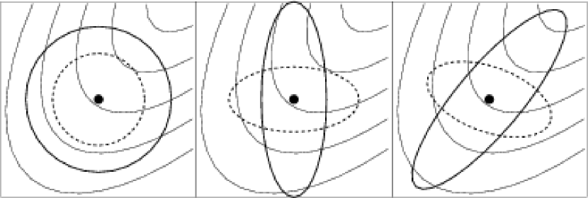
Figure 1: Examples of isotropic, uncorrelated, and correlated mutation distributions (indicated by circles, axis-parallel ellipsoids, and rotated ellipsoids, respectively) rendered over an elongated valley topography. The best average progress toward the topographic minimum in direction of the upper right corner is achieved in the right panel, where the mutation distribution (solid ellipsoid) is adapted to the topography

In contrast to the transition of parental vectors, there is no coherent conceptual scheme for the transition of the mutation operator $p^{(g)}$ from generation $g$ to $g+1$. However, due to basic considerations, any advanced transition scheme is expected to reflect the following elementary principles:

1. Invariance of the resulting ES with respect to any strictly monotone remapping of the range of the objective function as well as any linear transformation of the object parameter space. In particular, the resulting ES is expected to be unaffected by translation, rotation, and reflection.

2. Self-adaption of (the shape of) the mutation distribution to the topography of the objective function (Fig. 1). In particular, the mutation distribution is expected to reproduce the precedently selected mutation steps with increased likelihood.

The rigid implementation of these principles results in a concept of completely derandomized self-adaption where the transition of the mutation operator from one generation to the next is accomplished by successively updating the covariance matrix of the mutation distribution with information provided by the actually selected mutation step. The further demand of nonlocality involves the cumulation of the selected mutation steps into an evolution path.

2.2 Covariance matrix adaption (CMA)

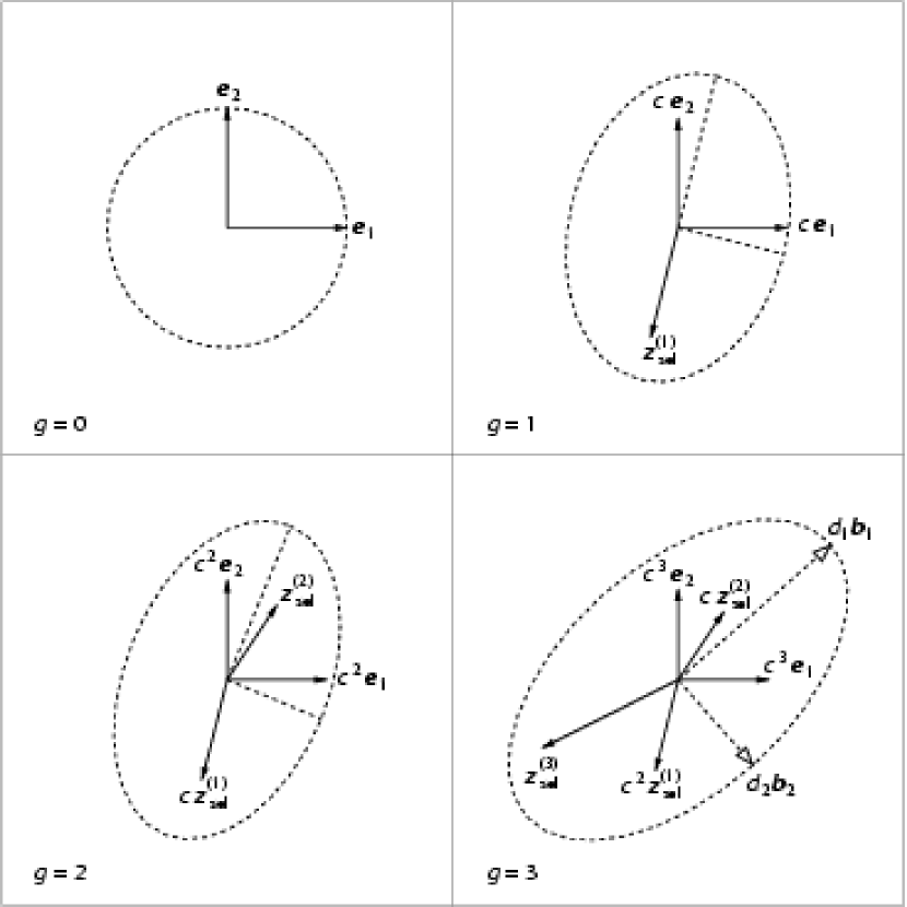
Figure 2: The conceptual scheme of covariance matrix adaption (CMA). Initially, the covariance matrix of the mutation distribution is $\@vec{C}^{(0)}=\@vec{e}_{1}\@vec{e}_{1}^{\mathrm{T}}+\@vec{e}_{2}\@vec{e}_{2}^{\mathrm{T}}$. In the course of the transition to the next generation $g+1$ the symmetric rank-one matrix $\@vec{z}^{(g+1)}_{\mathrm{sel}}(\@vec{z}^{(g+1)}_{\mathrm{sel}})^{\mathrm{T}}$, where $\@vec{z}^{(g+1)}_{\mathrm{sel}}$ is the actually selected mutation step, is added to the downscaled covariance matrix. In the third generation, the covariance matrix is $\@vec{C}^{(3)}=c^{6}\@vec{e}_{1}\@vec{e}_{1}^{\mathrm{T}}+c^{6}\@vec{e}_{2}\@vec{e}_{2}^{\mathrm{T}}+\sum_{i=1}^{3}c^{2(3-i)}\@vec{z}_{\mathrm{sel}}^{(i)}(\@vec{z}_{\mathrm{sel}}^{(i)})^{\mathrm{T}}=d_{1}^{2}\@vec{b}_{1}\@vec{b}_{1}^{\mathrm{T}}+d_{2}^{2}\@vec{b}_{2}\@vec{b}_{2}^{\mathrm{T}}$, where $\@vec{b}_{1}$ and $\@vec{b}_{2}$ are the unit eigenvectors of $\@vec{C}^{(3)}$ corresponding to the eigenvalues $d_{1}^{2}$ and $d_{2}^{2}$. The resulting mutation distribution reads $N(0,\@vec{C}^{(3)})=N(0,1)\,d_{1}\@vec{b}_{1}+N(0,1)\,d_{2}\@vec{b}_{2}$

If $\@vec{z}_{1},\dots,\@vec{z}_{m\in\mathbb{N}}\in\mathbb{R}^{n}$, $m\geq n$ are a generating set of $\mathbb{R}^{n}$ and $q_{1},\dots,q_{m}\in\mathbb{R}$ are a sequence of $(0,1)$-normally distributed random variables, then

$$q_{1}\@vec{z}_{1}+\dots+q_{m}\@vec{z}_{m}$$ (7)

renders an $n$-dimensional normal distribution with zero mean and covariance matrix

$$\@vec{z}_{1}\@vec{z}_{1}^{\mathrm{T}}+\dots+\@vec{z}_{m}\@vec{z}_{m}^{\mathrm{T}}.$$ (8)

In fact, Eq. (7) facilitates the realization of any normal distribution with zero mean. In particular, the symmetric rank-one matrix $\@vec{z}_{i}\@vec{z}_{i}^{\mathrm{T}}$ corresponds to that normal distribution with zero mean producing the vector $\@vec{z}_{i}$ with the maximum likelihood. Since the objective of CMA is to reproduce the precedently selected mutation steps with increased likelihood, the whole trick in order to accomplish this objective is to add the symmetric rank-one matrix

$$\@vec{z}^{(g+1)}_{\mathrm{sel}}(\@vec{z}^{(g+1)}_{\mathrm{sel}})^{\mathrm{T}},$$ (9)

where $\@vec{z}^{(g+1)}_{\mathrm{sel}}$ denotes the actually selected mutation step, to the covariance matrix of the mutation distribution. The conceptual scheme is illustrated in Fig. 2. Initially, the mutation distribution is isotropic

$$N(0,\@vec{C}^{(0)})=N(0,1)\,\@vec{e}_{1}+N(0,1)\,\@vec{e}_{2},$$ (10)

whereas in the course of the transition to the next generation the symmetric rank-one matrix Eq. (9) is added to the downscaled covariance matrix

$$\@vec{C}^{(g+1)}=c^{2}\@vec{C}^{(g)}+\@vec{z}_{\mathrm{sel}}^{(g+1)}(\@vec{z}_{\mathrm{sel}}^{(g+1)})^{\mathrm{T}},\quad c\in[0,1).$$ (11)

In the course of the third generation, for instance, the mutation distribution reads

$$N(0,\@vec{C}^{(3)}) = N(0,1)\,c^{3}\@vec{e}_{1}+N(0,1)\,c^{3}\@vec{e}_{2}+\sum_{i=1}^{3}N(0,1)\,c^{3-i}\@vec{z}_{\mathrm{sel}}^{(i)}$$ (12)

$$= N(0,1)\,d_{1}\@vec{b}_{1}+N(0,1)\,d_{2}\@vec{b}_{2},$$

where $\@vec{b}_{1}$ and $\@vec{b}_{2}$ are the unit eigenvectors of $\@vec{C}^{(3)}$ corresponding to the eigenvalues $d_{1}^{2}$ and $d_{2}^{2}$. Obviously, the mutation distribution tends to reproduce the precedently selected mutations steps. Finally, the mutation distribution becomes stationary (apart from scale) while its principal axes achieve conjugate perpendicularity, and $\@vec{C}^{(g)}$ effectively approaches the scaled inverse Hessian matrix of the objective function.

2.3 Evolution path cumulation

The efficiency as well as the stability of an ES improve significantly, if the decision of how to adapt the mutation distribution is based on the cumulation of several selected mutation steps rather than a single step. While the latter maximizes the local selection probability the former is more likely to advance the global progress rate. The benefit from superseding the successively selected mutation steps in favor of the evolution path

$$\@vec{p}^{(g+1)}=(1-c)\@vec{p}^{(g)}+\sqrt{c(2-c)}\@vec{z}_{\mathrm{sel}}^{(g+1)},\quad c\in(0,1]$$ (13)

is illustrated in detail in Paper A: If several successively selected mutation steps are parallel (antiparallel) correlated, the evolution path will be lengthened (shortened). If the evolution path is long (short), the size of the mutation steps in direction of the evolution path increases (decreases). The effect of cumulation is particularly beneficial in the case of small populations where the topographical information gathered within one generation is not sufficient. If $c=1$, no cumulation will occur and $\@vec{p}^{(g+1)}=\@vec{z}_{\mathrm{sel}}^{(g+1)}$.

2.4 The CMA evolution strategy (CMA-ES)

In this section we compile a unified formulation of the generic CMA-ES algorithms given in Papers A and B. In this form, the algorithm is not presented elsewhere. Besides the rank-one CMA outlined in the previous sections the algorithm features the advanced-rank CMA introduced in Paper B and an additional step size control. Finally, we conclude with remarks concerning the numerical implementation of the CMA-ES algorithm we provide online.

2.4.1 Generic algorithm

The state of the $(\mu,\lambda)$-CMA-ES in generation $g$ is defined by the family of parental vectors $\@vec{x}_{1}^{(g)},\dots,\@vec{x}_{\mu}^{(g)}\in\mathbb{R}^{n}$, the covariance matrix of the mutation distribution $\@vec{C}^{(g)}\in\mathbb{R}^{n\times n}$, the global mutation step size $\sigma^{(g)}\in\mathbb{R}^{+}$, and the evolution paths $\@vec{p}_{\mathrm{c}}^{(g)},\@vec{p}_{\sigma}^{(g)}\in\mathbb{R}^{n}$. The generic algorithm is completely defined by the transition from generation $g$ to $g+1$:

1. Weighted intermediate recombination of the parental vectors into the recombinant vector

   $$\langle\@vec{x}\rangle^{(g)}=\frac{\sum_{i=1}^{\mu}w_{i}\@vec{x}_{i}^{(g)}}{\sum_{i=1}^{\mu}w_{i}},\quad w_{1},\dots,w_{\mu}\in\mathbb{R}^{+}.$$ (14)

   The weights $w_{1},\dots,w_{\mu}$ are internal strategy parameters with canonical values

   $$w_{i}=\ln(\mu+1)-\ln(i),\quad i=1,\dots,\mu.$$ (15)

   The initial recombinant vector $\langle\@vec{x}\rangle^{(0)}$ is expected to enable the resulting mutation operator to sample the relevant part of the object parameter space.

2. Mutation of the recombinant vector to produce a new family of $\lambda>\mu$ offsprings

   $$\@vec{y}_{k}^{(g+1)}=\langle\@vec{x}\rangle^{(g)}+\sigma^{(g)}\@vec{B}^{(g)}\@vec{D}^{(g)}\@vec{z}_{k}^{(g+1)},\quad k=1,\dots,\lambda,$$ (16)

   where $\@vec{z}_{1}^{(g+1)},\dots,\@vec{z}_{\lambda}^{(g+1)}\in\mathbb{R}^{n}$ are a family of $(0,\@vec{I})$-normally distributed random vectors (i.e. the vector components are $(0,1)$-normally distributed), and $\@vec{D}^{(g)},\@vec{B}^{(g)}\in\mathbb{R}^{n\times n}$ diagonalize the covariance matrix

   $$\@vec{C}^{(g)}=\@vec{B}^{(g)}\@vec{D}^{(g)}\@vec{D}^{(g)}(\@vec{B}^{(g)})^{\mathrm{T}}.$$ (17)

   The elements of the diagonal matrix $\@vec{D}^{(g)}$ are the square roots of the eigenvalues of $\@vec{C}^{(g)}$, while the column vectors of $\@vec{B}^{(g)}$ are the corresponding unit eigenvectors. Constrained optimization can be realized by resampling $\@vec{z}_{1}^{(g+1)},\dots,\@vec{z}_{\lambda}^{(g+1)}$ until the constraints are satisfied.

3. Selection of the $\mu$ best individuals among the offspring population to become the next generation of parental vectors

   $$\@vec{x}^{(g+1)}_{i}=\@vec{y}^{(g+1)}_{i:\lambda},\quad i=1,\dots,\mu.$$ (18)

   Since the production of offsprings is independent of order the values of the objective function

   $$f(\@vec{y}_{k}^{(g+1)}),\quad k=1,\dots,\lambda$$ (19)

   can be computed in parallel.

4. Cumulation of the distribution evolution path

   $$\@vec{p}_{\mathrm{c}}^{(g+1)}=(1-c_{\mathrm{c}})\@vec{p}_{\mathrm{c}}^{(g)}+c_{w}\sqrt{c_{\mathrm{c}}(2-c_{\mathrm{c}})}\@vec{B}^{(g)}\@vec{D}^{(g)}\langle\@vec{z}\rangle^{(g+1)}$$ (20)

   with

   $$c_{w}=\frac{\sum_{i=1}^{\mu}w_{i}}{\sqrt{\sum_{i=1}^{\mu}w_{i}^{2}}}$$ (21)

   and

   $$\langle\@vec{z}\rangle^{(g+1)}=\frac{\sum_{i=1}^{\mu}w_{i}\@vec{z}^{(g+1)}_{i:\lambda}}{\sum_{i=1}^{\mu}w_{i}},$$ (22)

   where $\@vec{z}^{(g+1)}_{i:\lambda}$ follows from $\@vec{y}^{(g)}_{i:\lambda}$ by Eq. (16). The distribution cumulation rate $c_{\mathrm{c}}\in(0,1]$ is an internal strategy parameter with canonical value

   $$c_{\mathrm{c}}=\frac{4}{n+4}.$$ (23)

   If $c_{\mathrm{c}}=1$, no cumulation will occur. Initially, the distribution evolution path is $\@vec{p}_{\mathrm{c}}^{(0)}=0$.

5. Adaption of the covariance matrix

   $$\@vec{C}^{(g+1)} = (1-c_{\mathrm{cov}})\,\@vec{C}^{(g)}+c_{\mathrm{cov}}\left(\alpha_{\mathrm{cov}}\@vec{p}_{\mathrm{c}}^{(g+1)}(\@vec{p}_{\mathrm{c}}^{(g+1)})^{\mathrm{T}}\right.$$ (24)

   $$\phantom{(1-c_{\mathrm{cov}})\,\@vec{C}^{(g)}+c_{\mathrm{cov}}[}+\left.(1-\alpha_{\mathrm{cov}})\langle\@vec{Z}\rangle^{(g+1)}\right),$$

   where

   $$\langle\@vec{Z}\rangle^{(g+1)}=\frac{\sum_{i=1}^{\mu}w_{i}\@vec{B}^{(g)}\@vec{D}^{(g)}\@vec{z}_{i:\lambda}^{(g+1)}\left(\@vec{B}^{(g)}\@vec{D}^{(g)}\@vec{z}_{i:\lambda}^{(g+1)}\right)^{\mathrm{T}}}{\sum_{i=1}^{\mu}w_{i}}.$$ (25)

   The expressions $\@vec{p}_{\mathrm{c}}^{(g+1)}(\@vec{p}_{\mathrm{c}}^{(g+1)})^{\mathrm{T}}$ and $\langle\@vec{Z}\rangle^{(g+1)}$ are symmetric matrices of rank one and $\min(\mu,n)$, respectively, and generalize the conceptual scheme illustrated in Fig. 2 in case of a single parent ES. The parameter $\alpha_{\mathrm{cov}}\in[0,1]$ combines the two adaption mechanisms whereas $c_{\mathrm{cov}}\in[0,1)$ moderates the adaption rate. Both numbers are internal strategy parameters with canonical values

   $$\alpha_{\mathrm{cov}}=c_{w}^{-2}$$ (26)

   and

   $$c_{\mathrm{cov}}=\frac{2\alpha_{\mathrm{cov}}}{(n+\sqrt{2})^{2}}+(1-\alpha_{\mathrm{cov}})\,\operatorname{min}\left(1,\frac{2c_{w}^{2}-1}{(n+2)^{2}+c_{w}^{2}}\right).$$ (27)

   If $c_{\mathrm{cov}}=0$, no adaption will occur. Initially, $\@vec{C}^{(0)}=\@vec{I}$ or the square of any diagonal matrix properly scaling the optimization problem.

6. Cumulation of the step size evolution path

   $$\@vec{p}_{\sigma}^{(g+1)}=(1-c_{\sigma})\@vec{p}_{\sigma}^{(g)}+c_{w}\sqrt{c_{\sigma}(2-c_{\sigma})}\@vec{B}^{(g)}\langle\@vec{z}\rangle^{(g+1)},$$ (28)

   where the step size cumulation rate $c_{\sigma}\in(0,1]$ is an internal strategy parameter with canonical value

   $$c_{\sigma}=\frac{c_{w}^{2}+2}{n+c_{w}^{2}+3}.$$ (29)

   If $c_{\sigma}=1$, no cumulation will occur. Initially, the step size evolution path is $\@vec{p}_{\sigma}^{(0)}=0$.

7. Adaption of the global mutation step size

   $$\sigma^{(g+1)}=\sigma^{(g)}\,\exp\left(\frac{c_{\sigma}}{d_{\sigma}}\frac{\|\@vec{p}_{\sigma}^{(g+1)}\|-E_{n}}{E_{n}}\right),$$ (30)

   where the second fraction is the relative deviation of the length of $\@vec{p}_{\sigma}^{(g+1)}$ from its expected value in the case of no selection pressure, $E_{n}=\sqrt{2}\Gamma(\frac{n+1}{2})/\Gamma(\frac{n}{2})$, and the damping constant $d_{\sigma}\geq c_{\sigma}$ is an internal strategy parameter with canonical value

   $$d_{\sigma}=1+c_{\sigma}+2\operatorname{max}\left(0,\sqrt{\frac{c_{w}^{2}-1}{n+1}}-1\right).$$ (31)

   The initial mutation step size $\sigma^{(0)}$ is expected to enable the resulting mutation distribution to sample the relevant part of the object parameter space.

The impact and canonical setting of internal strategy parameters are discussed in detail in Paper A and Hansen & Kern (2004).

2.4.2 Numerical implementation

The numerical implementation of the CMA-ES algorithm is basically straightforward. We coded different function templates for both unconstrained and constrained optimization. The template instantiation requires a random number generator and an eigenvalue decomposition algorithm to be supplied as generic arguments. The numerical code is designed to perform in parallel when running on shared memory multiprocessing architectures and has been applied in practice by Quast et al. (2002, 2004) and Reimers et al. (2003).

Since an adequate random number generator producing high-dimensional equidistribution is absolutely essential to ensure the ES practically performs as expected in theory, we apply the Mersenne Twister algorithm furnishing equidistributed uniform deviates in up to 623 dimensions with period $2^{19937}-1$ (Matsumoto & Nishimura, 1998). The uniform deviates are converted into normal deviates by means of the polar method.

The Linear Algebra Package provides several algorithms suitable for diagonalizing the covariance matrix. For example, the routines decomposing tridiagonal matrices into relatively robust representations accurately complete the diagonalization of an $n\times n$ symmetric tridiagonal matrix in $O(n^{2})$ rather than the regular $O(n^{3})$ arithmetic operations (Dhillon & Parlett, 2004). In particular, it is feasible to diagonalize the covariance matrix just every $n/10$ generation to minimize the numerical overhead (Paper A). For, say, $n>10\,000$ using completely correlated mutation distributions will be impracticable and an ES algorithm calculating just the tridiagonal covariance matrix elements or adapting just individual step sizes ($\@vec{B}^{(g)}=\@vec{I}$, $\@vec{C}^{(g)}=\@vec{D}^{(g)}\@vec{D}^{(g)}$ diagonal) will be appropriate.

3 Spectral decomposition

In the case of pure line absorption, the observed spectral flux $F(\lambda)$ is modelled as the product of the continuum background and the instrumentally convoluted absorption term

$$F(\lambda)=C(\lambda)\int P(\xi)\,\mathrm{e}^{-\tau(\lambda-\xi)}\,\mathrm{d}\xi.$$ (32)

Defining

$$A(\lambda)=\int P(\xi)\,\mathrm{e}^{-\tau(\lambda-\xi)}\,\mathrm{d}\xi$$ (33)

and approximating the local continuum background by a linear combination of Legendre polynomials, Eq. (32) transforms into

$$F(\lambda)=\sum_{k}c_{k}\,L_{k}[\phi(\lambda)]A(\lambda),$$ (34)

where $L_{k}$ denotes the Legendre polynomial of order $k$, and $\phi$ is a linear map onto the interval $[-1,1]$. The instrumental profile $P(\xi)$ is modelled by a normalized Gaussian defined by the spectral resolution of the instrument. The instrumental convolution can be calculated piecewise analytically while approximating the absorption term with a polyline or a cubic spline. Without significant loss of accuracy, the integration can be restricted to the interval $|\xi|\leq 2\delta$, where $\delta$ is the full width at half maximum of the instrumental profile.

Presuming pure Doppler broadening, the optical depth $\tau$ is modelled by a superposition of Gaussian functions. If $\lambda_{i}$, $f_{i}$, $z_{i}$, $b_{i}$, $N_{i}$, and $\lambda_{z_{i}}=(1+z_{i})\lambda_{i}$ denote, respectively, the rest wavelength, the oscillator strength, the cosmological redshift, the line broadening velocity, the column density, and the observed wavelength corresponding to line $i$, then

$$\tau(\lambda)=\sum_{i}g_{i}(\lambda)$$ (35)

with

$$g_{i}(\lambda)=\frac{e^{2}}{4\varepsilon_{0}mc}\frac{N_{i}f_{i}\lambda_{i}}{\sqrt{\pi}b_{i}}\,\exp{\left[-\left(\frac{c}{b_{i}}\frac{\lambda-\lambda_{z_{i}}}{\lambda_{z_{i}}}\right)^{2}\right]}.$$ (36)

If natural broadening is important, the Gaussian functions will have to be replaced with Voigt functions. The latter can efficiently be calculated by using pseudo-Voigt approximations (Ida et al., 2000).

Taking the proper identification of lines for granted, the decomposition of an absorption line spectrum into individual profiles is a parametric inverse problem involving a tuple of three model parameters per line: position, broadening velocity, and column density. Given an observed set of spectral fluxes $F_{1},F_{2},\dots$ and normally distributed errors $\sigma_{1},\sigma_{2},\dots$ sampled at wavelengths $\lambda_{1},\lambda_{2},\dots$ the optimal parametric decomposition $F(\lambda)$ is calculated by minimizing the normalized residual sum of squares

$$\mathrm{RSS}=\sum_{j}\left(\frac{F_{j}-F(\lambda_{j})}{\sigma_{j}}\right)^{2}.$$ (37)

For any $A(\lambda)$, the minimization with respect to the coefficients $c_{k}$ presents a linear optimization problem

$$\mathrm{RSS}=\sum_{j}\left(\frac{F_{j}-\sum_{k}c_{k}\,L_{k}[\phi(\lambda_{j})]A(\lambda_{j})}{\sigma_{j}}\right)^{2}$$ (38)

which is solved directly by means of Cholesky decomposition. In the case of normally distributed errors the minimum RSS maximizes the likelihood.

Note that since the normalized RSS is invariant with respect to permutations of line parameter 3-tuples, any self-adaptive ES initially will require several generations to adapt to the symmetry. Any further global degeneracies of the search space will lengthen the initial adaption phase.

4 Performance tests

4.1 Test cases

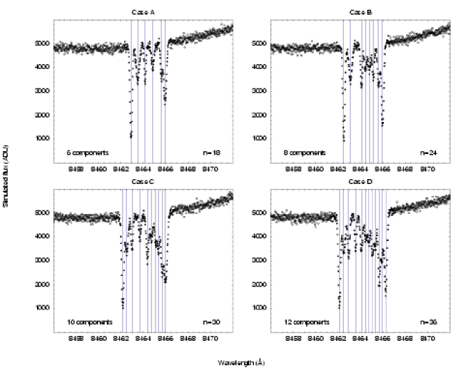
Figure 3: Artificial test cases based on an ensemble of intergalactic Ca ii $\lambda 3935$ lines toward the QSO HE 0515–4414. The simulated instrumental resolution is $R=60\,000$ while the simulated signal-to-noise ratio is about 50. Individual components are marked by vertical lines. The positional search space is indicated by solid dots

Table 1: Parameterization of the artificial lines used to synthesize the test cases rendered in Fig. 3. Rest wavelengths and oscillator strengths comply with the Ca ii $\lambda 3935$ transition. All CMA-ES runs converging at the global minimum result in the same parameterization indicated in parantheses, along with standard deviations provided by the diagonal elements of the scaled covariance matrix

Line	$z$	$b$ (km s-1)	$\log N$ (cm-2)
A-1	1.150800 (800)	3.0 ($2.9\pm 0.1$)	12.30 ($12.32\pm 0.01$)
A-2	1.150950 (949)	6.0 ($6.0\pm 0.2$)	11.80 ($11.80\pm 0.01$)
A-3	1.151120 (119)	2.5 ($1.9\pm 0.2$)	11.60 ($11.60\pm 0.02$)
A-4	1.151290 (290)	5.0 ($4.8\pm 0.3$)	11.50 ($11.51\pm 0.02$)
A-5	1.151490 (488)	3.0 ($2.8\pm 0.3$)	11.60 ($11.58\pm 0.02$)
A-6	1.151570 (569)	4.5 ($4.6\pm 0.2$)	12.00 ($12.01\pm 0.01$)
B-1	1.150700 (700)	3.0 ($2.9\pm 0.1$)	12.30 ($12.32\pm 0.01$)
B-2	1.150850 (850)	6.0 ($6.0\pm 0.2$)	11.80 ($11.80\pm 0.01$)
B-3	1.151100 (101)	2.5 ($2.5\pm 0.2$)	11.70 ($11.69\pm 0.01$)
B-4	1.151190 (189)	4.0 ($4.0\pm 0.5$)	11.50 ($11.50\pm 0.03$)
B-5	1.151280 (279)	5.5 ($5.6\pm 0.7$)	11.60 ($11.61\pm 0.03$)
B-6	1.151370 (370)	3.0 ($3.2\pm 0.3$)	11.60 ($11.60\pm 0.02$)
B-7	1.151490 (490)	4.5 ($4.4\pm 0.2$)	11.80 ($11.80\pm 0.01$)
B-8	1.151580 (580)	3.5 ($3.5\pm 0.1$)	12.20 ($12.20\pm 0.01$)
C-1	1.150610 (610)	3.0 ($2.9\pm 0.1$)	12.30 ($12.32\pm 0.02$)
C-2	1.150700 (701)	5.5 ($5.4\pm 0.3$)	11.80 ($11.79\pm 0.02$)
C-3	1.150820 (821)	3.0 ($2.8\pm 0.3$)	11.60 ($11.59\pm 0.02$)
C-4	1.151000 (000)	2.5 ($2.5\pm 0.4$)	11.40 ($11.38\pm 0.02$)
C-5	1.151170 (170)	4.0 ($3.9\pm 0.3$)	11.80 ($11.79\pm 0.02$)
C-6	1.151260 (261)	5.5 ($5.9\pm 0.8$)	11.60 ($11.61\pm 0.04$)
C-7	1.151360 (358)	3.5 ($3.2\pm 0.8$)	11.50 ($11.51\pm 0.07$)
C-8	1.151420 (421)	4.0 ($3.9\pm 0.8$)	11.70 ($11.71\pm 0.05$)
C-9	1.151500 (500)	3.5 ($3.3\pm 0.4$)	11.90 ($11.90\pm 0.03$)
C-10	1.151580 (579)	6.0 ($6.1\pm 0.2$)	12.20 ($12.21\pm 0.01$)
D-1	1.150600 (600)	3.0 ($3.0\pm 0.1$)	12.30 ($12.30\pm 0.01$)
D-2	1.150700 (700)	5.5 ($5.5\pm 0.2$)	11.80 ($11.81\pm 0.01$)
D-3	1.150810 (810)	3.0 ($3.0\pm 0.2$)	11.70 ($11.70\pm 0.01$)
D-4	1.150970 (968)	2.5 ($2.5\pm 0.2$)	11.60 ($11.59\pm 0.01$)
D-5	1.151100 (098)	4.0 ($4.1\pm 0.2$)	11.70 ($11.70\pm 0.02$)
D-6	1.151200 (203)	5.5 ($5.5\pm 1.0$)	11.60 ($11.60\pm 0.06$)
D-7	1.151270 (270)	3.0 ($2.8\pm 0.8$)	11.50 ($11.47\pm 0.08$)
D-8	1.151350 (347)	4.5 ($4.0\pm 0.6$)	11.80 ($11.77\pm 0.05$)
D-9	1.151420 (418)	3.5 ($4.6\pm 0.8$)	11.60 ($11.69\pm 0.06$)
D-10	1.151500 (500)	2.5 ($2.2\pm 0.3$)	12.00 ($12.00\pm 0.02$)
D-11	1.151560 (562)	5.0 ($5.3\pm 0.7$)	11.90 ($11.93\pm 0.04$)
D-12	1.151650 (651)	4.0 ($3.9\pm 0.1$)	12.20 ($12.19\pm 0.01$)

We have synthesized four exemplary test cases to investigate the global optimization performance of the CMA-ES when applied to the problem of spectral decomposition. The test cases are based on the characteristics of real QSO spectra and present a series of metal line ensembles increasing in complexity. Test cases A, B, C, and D render superpositions of six, eight, ten, and twelve components, respectively (Fig. 3). All test cases are synthesized simulating an instrumental resolution of $R=60\,000$ and a curved background continuum. Both Poissonian and Gaussian white noise are added producing a random continuum noise level of about two percent. Since ES are not destabilized by small scale oscillations of the objective function the complexity of the decomposition problem does not depend on the noise level of the data but is solely determined by the number and separation of spectral lines. The parameterization of the artificial lines used to synthesize the test cases is listed in Table 1. Several lines are barely separated or occcur close to the limit of the simulated spectral resolution.

The characteristics of the test cases are motivated by the analysis of QSO spectra recorded with the UV-Visual Echelle Spectropgraph installed at the Very Large Telescope. Further test cases exhibiting different characteristics will emerge in the future in course of the analysis of QSO spectra recorded with the Coudé Echelle Spectrograph operated at the ESO 3.6 m telescope. We do not consider line ensembles consisting of less than six components since these cases normally pose no challenge to the CMA-ES algorithm. Primitive cases exhibiting just a single component are completed in less than 50 generations using the canonical $(1,10)$-CMA-ES.

4.2 Algorithm application

We compare the global performance of the CMA-ES to that of several classical optimization algorithms provided by the Numerical Recipes collection: Fletcher-Reeves-Polak-Ribiere (FRPR, a conjugate gradient variant), Broyden-Fletcher-Goldfab-Shanno (BFGS, a virtual metric variant), Levenberg-Marquardt, Powell (a direction set variant), and the downhill simplex. The two latter algorithms do not require the calculation of partial derivatives and serve as direct standards of comparison.

The positional search space is restricted to an interval being 40 percent wider than the separation of the outer components (Fig. 3), while the broadening velocities and column densities are confined to $1.0\leq b\leavevmode\nobreak\ (\mathrm{km\,s}^{-1})\leq 10.0$ and $10.0\leq\log N\leavevmode\nobreak\ (\mathrm{cm}^{-2})\leq 14.0$. Since the classical algorithms are not prepared to handle simple parametric bounds per se, the Numerical Recipes routines are modified in such a way that any step attempting to escape is suppressed. The partial derivatives required by the FRPR, BFGS, and Levenberg-Marquardt algorithms are calculated numerically using the symmetrized difference quotient approximation.

Regarding the CMA-ES, we apply an $(100,200)$ algorithm with internal strategy parameters preset to the canonical values except for $\alpha_{\mathrm{cov}}=0$ and an increased covariance matrix adaption rate $c_{\mathrm{cov}}$. The diagonal elements of $\@vec{C}^{(0)}$ are initialized to the squared half widths of the parameter intervals while the mutation step size is initialized to $\sigma^{(0)}=0.5$.

For each algorithm and test case we monitor the history of 100 randomly initialized optimization runs. Providing the true number of absorption components as prior information, the initial object parameters are randomly drawn from a uniform distribution. The random noise is generated only once for each test case and is the same for all runs. All optimization runs are stopped after 100 000 evaluations of the normalized RSS.

4.3 Test results

The optimization runs are evaluated in terms of the ratio of the final normalized RSS to the normalized RSS corresponding to the true parameterization. For all test cases the RSS ratio is marginally less than unity at the global minimum. In general, an RSS ratio of unity just indicates the statistical consistency of the optimized and the true absorption profiles, but does not indicate the consistency of the optimized and the true parameterization. In particular in the case of QSO spectra exhibiting lower signal-to-noise ratios inconsistent optimized parameters will occur regularly. But however, since in our test cases the true parameterization is recovered by all runs converging at the global minimum (Table 1) the RSS ratio is appropriate to assess the global optimization performance. The outcome of optimization runs is summarized in Fig. 4 and Table 2 while Fig. 5 illustrates the performance of the CMA-ES during different stages of the optimization. In the following paragraphs the test results are described in detail.

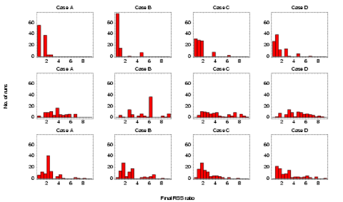
Figure 4: Outcome of 100 randomly initialized optimization runs using the CMA-ES (first row of histograms), Levenberg-Marquardt (second row), and Powell algorithms. The number of runs converging at the global minimum is indicated by the leftmost bar. The FRPR, BFGS, and simplex algorithms perform worse and are omitted for convenience

Table 2: Global optimization performance summarized in terms of the median of the final normalized RSS ratio, the number of runs converging at the global minimum, and the median number of RSS evaluations needed for that

Algorithm	Case A			Case B			Case C			Case D
CMA-ES	0.97	56	18 000	0.99	77	40 000	1.04	32	62 000	1.09	27	82 000
FRPR	4.86	2	36 000	9.45	3	70 000	6.65	–	–	11.7	–	–
BFGS	26.8	–	–	32.9	–	–	34.7	–	–	37.5	–	–
Levenberg-Marquardt	3.97	3	1000	6.11	–	–	4.24	–	–	5.04	–	–
Powell	2.12	6	14 000	2.67	2	20 000	2.05	2	26 000	2.69	–	–
Simplex	12.2	2	68 000	25.6	–	–	6.96	–	–	35.8	–	–

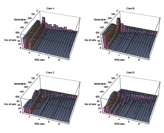
Figure 5: History of 100 randomly initialized optimization runs using the CMA-ES. The number of runs converging at the global minimum is indicated by the leftmost bar. The number of RSS evaluations is calculated by multiplying the generation number with 200

4.3.1 Case A

Case A consists of four isolated and two blended components. The lowest local minimum occurs when the weaker line of the blend is missed, but an isolated line is hit twice instead. Higher local minima occur whenever the blend is modelled correctly but any isolated component is missed. The CMA-ES hits the global minimum in 56 and the lowest local minimum in 38 runs. Another six runs converge at higher local minima while missing an isolated component. The most stable classical technique is the Powell algorithm, arriving at the global minimum in six, at the lowest local minimum in nine, and between these both in twelve runs. The most successful gradient technique is the Levenberg-Marquardt algorithm, reaching the global minimum in three runs. The latter algorithm also is the fastest, needing about 1000 evaluations of the normalized RSS to locate the global minimum, whereas the Powell and CMA-ES algorithms require about 14 000 and 18 000 evaluations, respectively. The FRPR and simplex algorithms hit the global minimum in two runs each, needing about 36 000 and 68 000 RSS evaluations, respectively. Except for the Powell algorithm the majority of deterministic runs misses two or more components. The BFGS algorithm never hits any component.

4.3.2 Case B

Case B is similar to case A but exhibits two additional components and a less narrow blend. The CMA-ES hits the global minimum in 77 and the lowest local minimum in 15 runs. Another eight runs converge at higher local minima. No deterministic algorithm locates the global minimum in more than three runs. The Powell algorithm is still relatively stable, missing one or two components in the majority of runs.

4.3.3 Case C

Case C again exhibits two additional components resulting in an ensemble of largely blended lines. The lowest local minimum occurs when the seventh component is missed, but another component is hit twice instead. The global minimum of the objective function almost has degenerated, being different from the lowest local minimum merely by seven percent. The CMA-ES hits the global minimum in 32 and the lowest local minimum in 22 runs. The majority of the remaining runs converges at higher local minima while missing a different one than the seventh component. The Powell algorithm hits the global as well as the lowest local minimum in 2 runs each and misses one or two components in the majority of runs. No further classical algorithm hits the global minimum.

4.3.4 Case D

Case D is very similar to case C but exhibits two additional components. The CMA-ES hits the global minimum in 27 runs. The majority of runs arrives at lower local minima without becoming stationary (Fig. 5). No classical algorithm hits the global minimum.

4.3.5 Efficiency

The number of RSS evaluations required by the CMA-ES to converge at the global minimum increases linearly with the number of lines superimposed in the test case (Table 2). The linear correlation coefficient is about $a=10\,000$ RSS evaluations per line. In case of the Powell algorithm the linear correlation coefficient is about $a=3000$.

5 Summary and conclusions

All tested classical algorithms require an adequate initial guess to locate the global optimum of the objective function when applied to the problem of spectral decomposition. In contrast, the CMA-ES is demonstrably capable to calculate the optimal decomposition without demanding any particular initialization, and therefore is just asking to be used in automatized spectroscopic analysis software.

The CMA-ES does not guarantee to find the optimal solution: characteristic spectral features are modelled correctly, but features exhibiting just a small attractor volume such as narrow components or tight blends are frequently not distinguished fittingly. Larger populations are expected to improve the chance to hit the global optimum but require a greater number of objective function evaluations. Peak finding algorithms could detect both the proper number (a problem that we have completely left aside) and position of spectral components and provide an improved initialization. But irrespective of whether an automatized analysis software will be realized, the CMA-ES is an elegant and highly competitive general purpose algorithm which is easy to implement. In our opinion, its integration into the standard astronomical data analysis packages will be thoroughly worthwhile and its widespread use will contribute to the further comprehension and improvement of suchlike algorithms.