Comments on the size of the simulation box in cosmological N-Body simulations

Abstract

N-Body simulations are a very important tool in the study of formation of large scale structures. Much of the progress in understanding the physics of high redshift universe and comparison with observations would not have been possible without N-Body simulations. Given the importance of this tool, it is essential to understand its limitations as ignoring the limitations can easily lead to interesting but unreliable results. In this paper we study the limitations arising out of the finite size of simulation volume. This finite size implies that modes larger than the size of the simulation volume are ignored and a truncated power spectrum is simulated. If the simulation volume is large enough then the mass in collapsed haloes expected from the full power spectrum and from the truncated power spectrum should match. We propose a quantitative measure based on this approach that allows us to compute the minimum box size for an N-Body simulation. We find that the required box size for simulations of $\Lambda$CDM model at high redshifts is much larger than is typically used. We can also use this approach to quantify the effect of perturbations at large scales for power law models and we find that if we fix the scale of non-linearity, the required box size becomes very large as the index becomes small. The appropriate box size computed using this approach is also an appropriate choice for the transition scale when tools like MAP [Tormen & Bertschinger, 1996] that add the contribution of the missing power are used.

1 Introduction

Large scale structures like galaxies and clusters of galaxies are believed to have formed by gravitational amplification of small perturbations [Peebles, 1980, Peacock, 1999, Padmanabhan, 2002, Bernardeau et al., 2002]. Observations suggest that the initial density perturbations were present at all scales that have been probed by observations. An essential part of the study of formation of galaxies and other large scale structures is thus the evolution of density perturbations for such initial conditions. The basic equations for this have been known for a long time [Peebles, 1974] and these equations are easy to solve when the amplitude of perturbations is small. Once the amplitude of perturbations at relevant scales becomes large, i.e., $\delta\sim 1$, the perturbation becomes non-linear and the coupling with perturbations at other scales cannot be ignored. The equation for evolution of density perturbations cannot be solved for generic perturbations in the non-linear regime. N-Body simulations [Bertschinger, 1998] are often used to study the evolution in this regime, unless one requires only a limited amount of information and quasi-linear approximation schemes [Zel’dovich, 1970, Gurbatov et al., 1989, Matarrese et al., 1992, Brainerd et al., 1993, Bagla & Padmanabhan, 1994, Sahni & Coles, 1995, Hui & Bertschinger, 1996, Bernardeau et al., 2002] or scaling relations [Davis & Peebles, 1977, Hamilton et al., 1991, Jain et al., 1995, Kanekar, 2000, Ma, 1998, Nityananda & Padmanabhan, 1994, Padmanabhan et al., 1996, Peacock & Dodds, 1994, Padmanabhan, 1996, Peacock & Dodds, 1996, Smith et al., 2003] suffice.

In N-Body simulations, we simulate a representative region of the universe. This representative region is a large but finite volume and periodic boundary conditions are often used – this is necessary considering the the universe does not have a boundary. Typically the simulation volume is taken to be a cube. Effect of perturbations at scales smaller than the mass resolution of the simulation, and of perturbations at scales larger than the box is ignored. Indeed, even perturbations at scales comparable to the box are under sampled. It has been shown that for gravitational dynamics in an expanding universe, perturbations at small scales do not influence collapse of large scale perturbations in a significant manner [Peebles, 1974, Peebles, 1985, Little et al., 1991, Bagla & Padmanabhan, 1997, Couchman & Peebles, 1998] as far as the correlation function or power spectrum at large scales are concerned. Therefore we may assume that ignoring perturbations at scales much smaller than the scales of interest does not affect results of N-Body simulations. However, there may be other effects that are not completely understood at the quantitative level [Bagla, Prasad, & Ray, 2004].

Perturbations at scales much larger than the simulation volume can affect the results of N-Body simulations. Use of periodic boundary conditions implies that the average density in the simulation box is same as the average density in the universe, in other words we are assuming that there are no perturbations at the scale of the simulation volume (or at larger scales). Therefore the size of the simulation volume should be chosen so that the amplitude of fluctuations at that scale (and at larger scales) is ignorable. If the amplitude of perturbations at larger scales is not ignorable and the simulations do not take the contribution of these scales into account then clearly the simulation will not be a faithful representation of the model being simulated. It is not obvious as to when fluctuations at larger scales can be considered ignorable. In this paper we will propose one method of quantifying this concept.

If the amplitude of density perturbations at the box scale is small but not ignorable, simulations underestimate the correlation function though the number density of small mass haloes does not change by much [Gelb & Bertschinger, 1994a, Gelb & Bertschinger, 1994b]. In other words, the formation of small haloes is not disturbed but their distribution is affected by non-inclusion of long wave modes. The mass function of massive haloes changes significantly [Gelb & Bertschinger, 1994a, Gelb & Bertschinger, 1994b]. The void spectrum is also affected by finite size of the simulation volume if perturbations at large scales are not ignorable [Kauffmann & Melott1992].

Significance of perturbations at large scales has been discussed in detail and a method (MAP) has been devised for incorporating the effects of these perturbations [Tormen & Bertschinger, 1996]. These methods make use of the fact that if the box size is chosen to be large enough then the contribution of larger scales can be incorporated by adding displacements due to the larger scales independently of the evolution of the system in an N-Body simulation. But this again brings up the issue of what is a large enough scale in any given model such that these methods can be used to add the effect of larger scales without introducing errors. Large scales contribute to displacements and velocities, and variations in density due to these scales modify the rate of growth for small scales perturbations [Cole, 1997]. The MAP algorithm [Tormen & Bertschinger, 1996] can be improved by adding corrections for this effect [Cole, 1997]. The motivation for developing these tools was to enlarge the dynamic range over which results of N-Body simulations are valid by adding corrections that change the distribution of matter and velocities at scales comparable to the simulation volume.

Name	$N_{p}$	$L_{box}$	$\epsilon$	Cutoff
T_300_C_0	$256^{3}$	$300$h-1Mpc	$0.47$h-1Mpc	No
T_300_C_2	$256^{3}$	$300$h-1Mpc	$0.47$h-1Mpc	$k\leq 2k_{f}$
T_300_C_3	$256^{3}$	$300$h-1Mpc	$0.47$h-1Mpc	$k\leq 3k_{f}$
T_300_C_4	$256^{3}$	$300$h-1Mpc	$0.47$h-1Mpc	$k\leq 4k_{f}$

Table 1: This table lists parameters of N-Body simulations we have used. All the simulations were done using the TreePM code, configuration described in Bagla and Ray (2003). We simulated the $\Lambda$CDM model with $\Omega_{B}=0.05$, $\Omega_{dm}=0.3$, $k=0$, $h=0.7$ and $n=1$. The first column lists name of the simulation, second column lists the number of particles in the simulation, the third column is the size of the box in physical units, fourth column lists the softening length for force and the last column lists the cutoff used in units of the fundamental mode of the box $k_{f}$. Phases were kept the same for the simulations listed here in order to make the comparison meaningful.

Our motivation in this work is to understand the effect of large scales on scales that are much smaller than the simulation volume. We run a series of numerical experiments, these are described in §2. We discuss the proposed method of quantifying the effect of large scales in §3. Here, we propose a measure based on mass functions. The minimum size of simulation volume for $\Lambda$CDM model as a function of redshift is presented here.

2 N-Body Simulations

We carried out two series of N-Body experiments in order to study the effect of perturbations at large scales on perturbations at small scales. The simulations were carried out using the TreePM method [Bagla, 2002, Bagla & Ray, 2003] and its parallel version [Ray & Bagla, 2004]. We simulated the $\Lambda$CDM model with $\Omega_{B}=0.05$, $\Omega_{dm}=0.3$, $\Omega_{tot}=1$, $h=0.7$ and $n=1$. In each of these series of simulations we ran a simulation without any truncation of the power spectrum, save those imposed by the finite size and resolution of the simulation box. These simulations served as a reference for other simulations where we truncated the power spectrum at small wave numbers. We used a sharp cutoff such that the power spectrum at $k\leq k_{c}$ was taken to be zero. A comparison of these simulations allows us to estimate the effect of density perturbations at large scales on growth of perturbations at small scales. Detailed specifications of these simulations are listed in table 1 where the cutoff wave number is listed in the units of the fundamental mode $k_{f}=2\pi/L_{box}$ of the simulation box.

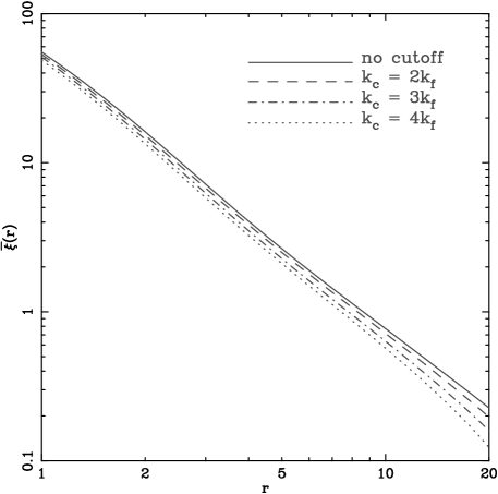
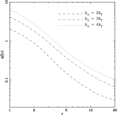
Figure 1: The top panel shows the averaged correlation function $\bar{\xi}$ as a function of $r$ for the models listed in table 1. The amplitude of the correlation function decreases as cutoff becomes smaller. The lower panel shows the deviation of $\bar{\xi}$ for models with an explicit cutoff from the simulation T_300_C_0. The correlation function is underestimated by about $10\%$ at $r=2$h^-1Mpc for a cutoff of $100$h^-1Mpc.

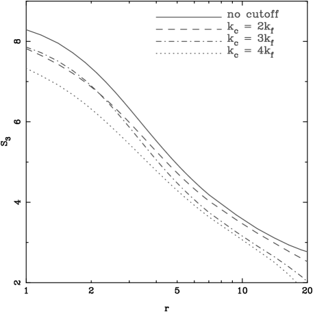
Figure 2: This figure shows the skewness $S_{3}$ as a function of $r$ for the models listed in table 1. The skewness decreases sharply as cutoff becomes smaller.

We compare the output of these simulations to see whether retaining or dropping long wave modes affects quantities of interest at smaller scales. Nearly all the comparisons we carry out will concentrate on scales smaller than $20$h^-1Mpc whereas the smallest cutoff we use is $75$h^-1Mpc, so the two sets of scales are well separated in most cases we consider here. The amplitude of root mean square fluctuations in mass at $r=75$h^-1Mpc and $z=0$ is $\sigma\sim 0.05$ in the model considered here and we can certainly consider this to be small.

Figure 1 shows the averaged correlation function $\bar{\xi}$ as a function of $r$ at $z=0$ for the models listed in table 1. The amplitude of the correlation function decreases as cutoff becomes smaller. The shape of the correlation function does not change at small scales. This result follows expectations and is indeed similar to figure 2 in [Gelb & Bertschinger, 1994b]. Thus the overall effect of perturbations at very large scales is to enhance the amplitude of fluctuations at smaller scales. Ignoring larger scales leads to an underestimate of correlation function at small scales. The correlation function is underestimated by $10\%$ at $r=2$h^-1Mpc for a cutoff of $100$h^-1Mpc. At this scale, $\sigma=0.04$ for $z=0$ in the model we have simulated. If we were to compute the linearly extrapolated $\bar{\xi}$ then the difference between the model with and without cutoff is much smaller than $10\%$. We have plotted the skewness $S_{3}$ as a function of scale in figure 2 for the same set of models. The difference in models here is significant. It is clear from these two figures that fairly large scales ($l\leq 100$h^-1Mpc) make a significant contribution to clustering at small scales ($l\leq 10$h^-1Mpc).

It is possible to correct for the contribution of larger scales for moments of particle distribution [Colombi et al., 1994]. Thus if we are interested only in the moments then we can circumvent this problem and compute the correct answer. There are many quantities of interest other than the moments of distribution and there is no generic method for computing the corrections and take the effect of large scales into account.

A method has been devised to incorporate the effect of displacements and velocities contributed by large scales [Tormen & Bertschinger, 1996]. Here, displacements and velocities contributed by larger scales are computed using the Zel’dovich approximation [Zel’dovich, 1970] and added to the numbers computed in the N-Body simulations. Essentially this assumes that there is no coupling in velocity contributed by modes within the box and modes larger than the box. With this assumption, other methods for computing the displacement due to modes outside the box can also be used in place of the Zel’dovich approximation. The assumption of no mode coupling is true only in the linear regime and hence we still require the amplitude of perturbations at the scale of the simulation box to be much smaller than unity. How small the amplitude should be can only be determined by trial and error. It has been pointed out that the effect of mode coupling can be emulated by enhancing the displacements without modifying the velocities [Cole, 1997]. The amount of enhancement needed cannot be derived from first principles. These tools essentially enhance the dynamic range on an N-Body simulation by making these corrections, displacements due to large scales correct the velocity fields at scales comparable to the simulation volume.

Corrections to displacements and velocities can be made without worrying about mode coupling if their effect is small in some absolute sense. An important fact to keep in mind is that none of these methods can be effective if the displacements contributed by large scale modes move two collapsed objects to the same location, or move matter that has fallen into a collapsed structure out of it. If the contribution of modes that can affect collapsed structures is not taken into account then the properties of these objects, e.g. mass, angular momentum, density profile, etc., may differ significantly from their asymptotic values. This is illustrated in figure 3. This figure shows the projected particle distribution in the neighbourhood of a massive cluster from simulations of the $\Lambda$CDM model. Four panels correspond to the models listed in table 1. The total mass in the central massive halo decreases as the large scale cutoff is introduced and then decreased. The number, masses and the distribution of smaller clumps around the central clump also change significantly as the cutoff is reduced below $150$h^-1Mpc.

Figure 4 shows the fraction of mass in collapsed structures with mass greater than $M$ for the models listed in table 1. This fraction is plotted as a function of mass $M$. The solid curve shows $F(>M)$ for the simulation without an explicit cutoff, of course there is an implicit cutoff at the box size ($300$h^-1Mpc). Other curves mark the function for different values of the cutoff and as the cutoff scale becomes smaller $F(>M)$ decreases at large $M$. At smaller masses ($M\leq 10^{14}$M_⊙), the difference in models is negligible. Difference between different curves at the high mass ($M\simeq 10^{15}$M_⊙) end is significant, more than a factor two between the extreme curves. Thus ignoring large scale modes results in an underestimate of the number of massive haloes. $F(>M)$ varies rapidly up to a cutoff of $150$h^-1Mpc and changes very little as the cutoff moves to larger scales. We may conclude from here that scales larger than $150$h^-1Mpc do not contribute significantly to collapsed structures in the currently favoured $\Lambda$CDM models.

Figure 3: Four panels of this figure show the projected particle distribution in the neighbourhood of a massive cluster from simulations of the $\Lambda$CDM model. The top left panel is for the first simulation in table 1, top right panel is for the second simulation, lower left panel is for the third simulation and the lower right panel is for the fourth simulation in the table. The total mass in the central massive halo decreases as the large scale cutoff is introduced and then decreased. The number, masses and the distribution of smaller clumps around the central clump also change significantly as the cutoff is reduced below $150$h^-1Mpc.

3 The Proposed Criterion

In the previous section we have argued that the non-trivial contribution of large scale modes is the one that leads to collapse of haloes, other effects like displacements can be incorporated, in principle, using algorithms like MAP [Tormen & Bertschinger, 1996, Cole, 1997]. We can use this to devise a criterion to decide whether the box size of a simulation is sufficiently large or not.

The collapsed mass fraction in haloes of mass $M$ or larger is given by [Press & Schechter, 1974, Bond et al., 1991]

$$F(M,z)={\rm erfc}\left[\frac{\delta_{c}}{\sqrt{2}\sigma_{L}\left(M,z\right)}\right]$$ (1)

The parameter $\delta_{c}$ indicates the linearly extrapolated density contrast at which the perturbation is expected to collapse and virialise in non-linear spherical collapse, its value is taken to be $1.686$ here. The precise value of this parameter is not very relevant here. Here $\sigma(M,z)$ is the root mean square (rms) amplitude of fluctuations at the mass scale $M$ and redshift $z$.

$$\sigma_{L}^{2}(M,z) = 9D_{+}^{2}(z)\int\limits_{0}^{\infty}\frac{dk}{k}\frac{k^{3}P(k)}{2\pi^{2}}\left[\frac{\sin{kr}-kr\cos{kr}}{k^{3}r^{3}}\right]^{2}$$

$$M = \frac{4\pi}{3}{\bar{\rho}}r^{3}$$ (2)

Here $P(k)$ is the power spectrum of density fluctuations, linearly extrapolated to $z=0$ and $D_{+}(z)$ is the growing mode in the linear perturbation theory normalised so that $D_{+}(z=0)=1$. The average matter density in the universe is denoted by $\bar{\rho}$.

In an N-Body simulation, the initial conditions sample a range of values of wave number $k$. The amplitude of rms fluctuations in the simulation will be different due to partial sampling of modes. The periodic boundary conditions restrict us to a discrete set of wave numbers in the range of scales studied and sampling is partial due to sparse sampling of $k-$space at scales comparable to the size of the simulation volume. Wave numbers smaller than the fundamental mode of the simulation volume are not sampled, nor are wave numbers larger than the Nyquist frequency of the mesh used for generating initial conditions. From the form of the integral it is clear that at a given scale $r$, wave modes with $k\leq 2\pi/r$ contribute more significantly than the rest. Given this and the fact that most modern N-Body simulations have sufficient dynamic range, we can concentrate on the lower limit of the range of wave numbers sampled in an N-Body simulation as modes with $k\geq k_{max}$ do not influence scales resolved in the simulation in any significant manner. We can then estimate the rms fluctuations in N-Body simulations by changing the lower limit of the integral in eqn.(2) from $0$ to $2\pi/L_{box}$ while leaving the upper limit unchanged. The fluctuations will now be a function of the cutoff as well:

$$\sigma_{L}^{2}(M,z,L_{box})=9D_{+}^{2}(z)$$

$$\;\;\;\;\;\;\;\;\;\;\times\int\limits_{2\pi/L_{box}}^{\infty}\frac{dk}{k}\frac{k^{3}P(k)}{2\pi^{2}}\left[\frac{\sin{kr}-kr\cos{kr}}{k^{3}r^{3}}\right]^{2}$$ (3)

We can use this in eqn.(1) and obtain $F(M,z,L_{box})$, the expected collapsed mass fraction in an N-Body simulation. Here we have approximated the sum over the discrete set of $k-$modes by an integral and assumed that the upper limit on the wave numbers sampled is less relevant for estimating the mass function at scales of interest.

In the previous section we found that in N-Body simulations the collapsed mass fraction does not change much if the cutoff is larger than $150$h^-1Mpc. This conclusion is reaffirmed by the theoretical calculation of the mass function and collapsed mass fraction. Figure 5 shows $F(M,L_{box})$ as a function of mass $M$ for different values of the cutoff scale $L_{box}$. The mass in the most massive collapsed structures changes rapidly with the cutoff, implying that the number density of most massive structures depends strongly on the large scale modes. Comparison with figure 4 shows that the theoretical calculation and simulations give comparable results.

The criterion we propose here is this: the physical scale $L_{box}$ corresponding to the size of the simulation volume can be considered to be large enough if the expected fraction of mass in haloes $F(M,z,L_{box})$ is comparable to $F(M,z)$, the fraction of mass in haloes when the full spectrum is taken into account. In other words, we require convergence of expected mass in haloes for the simulation volume to be considered large enough so that all the relevant scales are contained within it. As before, we are interested in the effect of large scales on scales much smaller than $L_{box}$. Therefore we wish to see this convergence at mass scales of typical haloes. We define the mass scale of non-linearity as $\sigma_{L}(M_{*},z)=1$ and study the convergence of mass function at this scale and at neighbouring mass scales.

We study two masses for the $\Lambda$CDM model: $M_{*}$ and $10M_{*}$. As we shall see, these are more relevant than smaller mass scales in most situations. We require $F(M,z,L_{box})=(1-\epsilon)F(M,z)$ to find the threshold length scale $L_{box}$, with $\epsilon=0.05$ and a less conservative limit of $\epsilon=0.1$. These criteria allow us to develop a feel for this approach. We certainly require a reasonable convergence at the scale of non-linearity in simulations. For some applications, as when studying rich clusters of galaxies, we require good convergence for very massive haloes. Figure 6 shows $L_{box}$ as a function of redshift $z$ according to these criteria for the $\Lambda$CDM model (see §2 for the values of cosmological parameters). The solid curve ($\epsilon=0.1$) and the dot-dashed curve ($\epsilon=0.05$) are for $M=M_{*}$, the dashed curve ($\epsilon=0.1$) and the dotted curve ($\epsilon=0.05$) are for $M=10M_{*}$. For the $\Lambda$CDM model, $M_{*}(z=0)=1.2\times 10^{14}$M_⊙ therefore the criteria used here refer to mass scales of typical clusters of galaxies and rich clusters of galaxies, respectively, at redshift $z=0$. At $z=0$, it is clear that a box larger than $100$h^-1Mpc is required even if we are interested in haloes with mass $M_{*}$ and can tolerate an offset of $10\%$ in collapsed mass. Using a smaller box size leads to a greater underestimate of the collapsed mass in haloes. The requirement becomes more stringent if we wish to study rich clusters of galaxies or use a tolerance level of $5\%$ ($\epsilon=0.05$).

Figure 4: This figure shows the fraction of mass in collapsed structures with mass greater than $M$ for the models listed in table 1. While the change in cutoff does not change the collapsed mass fraction for $M\leq 10^{14}$M_⊙, the collapsed fraction is underestimated at larger masses when we remove the large scale modes. Suppression of mass function around $M=10^{15}$M_⊙ is significant when the cutoff is at scales smaller than $150$h^-1Mpc.

Figure 5: This figure shows the fraction of mass in collapsed structures with mass greater than $M$ for the $\Lambda$CDM model used here. This was computed using the Press-Schechter mass function (Press & Schechter, 1974). A cutoff was used to remove contributions from large scales (see §3 for details). Note that these values of cutoff coincide with those used in simulations of models listed in table 1 and plotted in figure 4.

Figure 6: We have plotted $L_{box}$ as a function of redshift $z$ for the $\Lambda$CDM model (see §2 for the values of cosmological parameters). Using a smaller box size than outlined here leads to a greater underestimate of the collapsed mass in haloes than given by conditions used for these curves.

At $z=3$, $M_{*}=1.2\times 10^{11}$M_⊙. This is the mass of a typical galaxy halo at that redshift and to get the statistics of these objects right we should have a box size of at least $30$h^-1Mpc ($\epsilon=0.1$), the required box size increases to $50$h^-1Mpc if we require $\epsilon=0.05$ instead. This, or an even larger simulation box should be used if we wish to study the inter-galactic medium as there will be more matter left in uncollapsed regions if we use a smaller simulation box. Bright Lyman break galaxies are likely to be in more massive than typical haloes and a box size of $60$h^-1Mpc or larger is needed to study these in an N-Body simulation.

At higher redshifts, simulations are often used for studying reionisation of the universe. At $z=10$, $M_{*}=2\times 10^{6}$M_⊙. Sources of ionising radiation are likely to reside in much more massive haloes and hence we should use a simulation box that is at least $20$h^-1Mpc across ($M=10M_{*}$ and $\epsilon=0.05$). If we relax the requirement to $\epsilon=0.1$ then the simulation volume should be more than $10$h^-1Mpc across. Of course, very high peaks that may be the first sources of ionising radiation are rare and a very large simulation box is required to study patchiness in ionising radiation and hence reionisation [Barkana & Loeb2004].

Clearly, the requirement that the mass in collapsed haloes should not depend significantly on scales larger than the simulation box is fairly stringent and in some cases it may make it difficult to address the physical problem of interest. This restriction is less stringent than requiring that the correlation function of haloes converge as it has been shown that the mass function converges well before the correlation function of haloes [Gelb & Bertschinger, 1994a, Gelb & Bertschinger, 1994b]. However, if the mass function has converged then tools like MAP [Tormen & Bertschinger, 1996] can be used to obtain the correct distribution of haloes. Of course, curves can be drawn with different requirements on the convergence of collapsed mass as long as these requirements are in consonance with the physical application for which the simulation is being run.

Figure 7: $L_{box}$ is shown as a function of the index of power spectrum for power law models, $P(k)=Ak^{n}$. The power spectrum is normalised such that $\sigma_{L}(r=1)=1$. We have assumed an Einstein-de Sitter background for these models. It is clear from this figure that it is difficult to explore the highly non-linear regime for smaller values of $n$.

The curves for $\epsilon=0.1$ are not parallel to the curves for $\epsilon=0.05$, this is due to a dependence on the shape of the power spectrum. This dependence is brought out very clearly in figure 7. Here we show $L_{box}$ as a function of the index of power spectrum for power law models, $P(k)=Ak^{n}$. The power spectrum is normalised such that $\sigma_{L}(r=1)=1$. We have assumed an Einstein-de Sitter background for these models. The solid curve ($\epsilon=0.1$) and the dot-dashed curve ($\epsilon=0.05$) are for $M=M_{*}$, the dashed curve ($\epsilon=0.1$) and the dotted curve ($\epsilon=0.05$) are for $M=5M_{*}$. It is clear from this figure that it is difficult to explore the highly non-linear regime for smaller values of $n$, required box size increases rapidly as $(n+3)\rightarrow 0$.

These figures show that the convergence of collapsed mass in haloes happens slowly for most models of interest. The offset in collapsed mass for the the simulated model (with a finite sampling of scales) from the collapsed mass for the model that we wish to simulate is a useful indicator of the relevance of large scales. This feature allows us to use the criterion to decide the size of the simulation volume; the criterion supplies the lower bound on the size.

4 Conclusions

We have studied the influence of long wave modes on gravitational clustering at small scales. We find that for the $\Lambda$CDM model, scales larger than $100$h^-1Mpc affect the mass function of haloes and the distribution of matter at scales as small as a few Mpc. The effect of long wave modes not present in an N-Body simulation can be incorporated independently of the evolution at small scales for some quantities but making such corrections is not possible in general. In particular, it is not possible to make corrections if the contribution of large scales changes the mass of collapsed haloes by a significant amount. We can turn this argument around and check whether a given size of the simulation volume will give (close to) correct results for total collapsed mass in haloes or not. This can be done using simple analytical formulae outlined in §3. The fractional deviation of collapsed mass from its expected value if density fluctuations at all scales are taken into account is a good indicator of the influence of large scales. The fractional deviation ($\epsilon$) can be checked at a given mass scale $M$ of physical interest. Given a choice of $M$, $\epsilon$ and the redshift $z$ at which output of the simulation is to be studied, we can compute the recommended minimum size for the simulation volume. It is important to note that this scale is the minimum required and a larger simulation may be warranted by other requirements.

The mass in collapsed haloes converges faster than the correlation function of haloes, implying that an even larger simulation volume may be required. Corrections to positions and velocities due to large scales can be made using tools such as MAP [Tormen & Bertschinger, 1996, Cole, 1997]. Thus we can choose the box size by requiring convergence of mass in haloes and then use MAP to get the correct distribution and velocity field at all scales. Of course, if MAP is not being used then a larger box size than the minimum indicated by convergence of mass function may be required. Of course, using a large box size can make it difficult to address interesting questions using N-Body simulations. We believe that it is better to be cautious rather than obtain unreliable answers, unless one can make a convincing case that the relevant physical quantities are not as sensitive as mass in collapsed haloes to the size of the simulation box.

References

- [Bagla, 2002] Bagla J. S., 2002, Journal of Astrophysics and Astronomy, 23, 185, astro-ph/9911025
- [Bagla & Padmanabhan, 1994] Bagla J. S., Padmanabhan T., 1994, MNRAS, 266, 227
- [Bagla & Padmanabhan, 1997] Bagla J. S., Padmanabhan T., 1997, MNRAS, 286, 1023
- [Bagla & Ray, 2003] Bagla J. S., Ray S., 2003, New Astronomy, 8, 665
- [Bagla, Prasad, & Ray, 2004] Bagla J. S., Prasad J., Ray S., 2004, astro-ph/0408429
- [Barkana & Loeb2004] Barkana R., Loeb A., 2004, ApJ, 609, 474
- [Bernardeau et al., 2002] Bernardeau F., Colombi S., Gaztañaga E., Scoccimarro R., 2002, Physics Reports, 367, 1
- [Bertschinger, 1998] Bertschinger E., 1998, ARA&A, 36, 599
- [Bond et al., 1991] Bond J. R., Cole S., Efstathiou G., Kaiser N., 1991, ApJ, 379, 440
- [Brainerd et al., 1993] Brainerd T. G., Scherrer R. J., Villumsen J. V., 1993, ApJ, 418, 570
- [Cole, 1997] Cole S., 1997, MNRAS, 286, 38
- [Colombi et al., 1994] Colombi S., Bouchet F. R., Schaeffer R., 1994, A&A, 281, 301
- [Couchman & Peebles, 1998] Couchman H. M. P., Peebles P. J. E., 1998, ApJ, 497, 499
- [Davis & Peebles, 1977] Davis M., Peebles P. J. E., 1977, ApJS, 34, 425
- [Gelb & Bertschinger, 1994a] Gelb J. M., Bertschinger E., 1994a, ApJ, 436, 467
- [Gelb & Bertschinger, 1994b] Gelb J. M., Bertschinger E., 1994b, ApJ, 436, 491
- [Gurbatov et al., 1989] Gurbatov S. N., Saichev A. I., Shandarin S. F., 1989, MNRAS, 236, 385
- [Hamilton et al., 1991] Hamilton A. J. S., Kumar P., Lu E., Matthews A., 1991, ApJL, 374, L1
- [Hui & Bertschinger, 1996] Hui L., Bertschinger E., 1996, ApJ, 471, 1
- [Jain et al., 1995] Jain B., Mo H. J., White S. D. M., 1995, MNRAS, 276, L25
- [Kanekar, 2000] Kanekar N., 2000, ApJ, 531, 17
- [Kauffmann & Melott1992] Kauffmann G., Melott A. L., 1992, ApJ, 393, 415
- [Little et al., 1991] Little B., Weinberg D. H., Park C., 1991, MNRAS, 253, 295
- [Ma, 1998] Ma C., 1998, ApJL, 508, L5
- [Matarrese et al., 1992] Matarrese S., Lucchin F., Moscardini L., Saez D., 1992, MNRAS, 259, 437
- [Nityananda & Padmanabhan, 1994] Nityananda R., Padmanabhan T., 1994, MNRAS, 271, 976
- [Padmanabhan, 1996] Padmanabhan T., 1996, MNRAS, 278, L29
- [Padmanabhan, 2002] Padmanabhan T., 2002, Theoretical Astrophysics, Volume III: Galaxies and Cosmology. Cambridge University Press.
- [Padmanabhan et al., 1996] Padmanabhan T., Cen R., Ostriker J. P., Summers F. J., 1996, ApJ, 466, 604
- [Peacock, 1999] Peacock J. A., 1999, Cosmological physics. Cambridge University Press.
- [Peacock & Dodds, 1994] Peacock J. A., Dodds S. J., 1994, MNRAS, 267, 1020
- [Peacock & Dodds, 1996] Peacock J. A., Dodds S. J., 1996, MNRAS, 280, L19
- [Peebles, 1974] Peebles P. J. E., 1974, A&A, 32, 391
- [Peebles, 1980] Peebles P. J. E., 1980, The large-scale structure of the universe. Princeton University Press.
- [Peebles, 1985] Peebles P. J. E., 1985, ApJ, 297, 350
- [Press & Schechter, 1974] Press W. H., Schechter P., 1974, ApJ, 187, 425
- [Ray & Bagla, 2004] Ray S., Bagla J. S., 2004, astro-ph/0405220
- [Sahni & Coles, 1995] Sahni V., Coles P., 1995, Physics Reports, 262, 1
- [Sheth & Tormen, 1999] Sheth R. K., Tormen G., 1999, MNRAS, 308, 119
- [Smith et al., 2003] Smith R. E., Peacock J. A., Jenkins A., White S. D. M., Frenk C. S., Pearce F. R., Thomas P. A., Efstathiou G., Couchman H. M. P., 2003, MNRAS, 341, 1311
- [Tormen & Bertschinger, 1996] Tormen G., Bertschinger E., 1996, ApJ, 472, 14
- [Zel’dovich, 1970] Zel’dovich Y. B., 1970, A&A, 5, 84