Spectral disentangling of the triple system DG Leo: orbits and chemical composition

Abstract

DG Leo is a spectroscopic triple system composed by 3 stars of late-A spectral type, one of which was suggested to be a $\delta$ Scuti star. Seven nights of observations at high spectral and high time resolution at the Observatoire de Haute-Provence with the ELODIE spectrograph were used to obtain the component spectra by applying a Fourier transform spectral disentangling technique. Comparing these with synthetic spectra, the stellar fundamental parameters (effective temperature, surface gravity, projected rotation velocity and chemical composition) are derived. The inner binary consists of two Am components, at least one of which is not yet rotating synchronously at the orbital period though the orbit is a circular one. The distant third component is confirmed to be a $\delta$ Scuti star with normal chemical composition.

1 Introduction

Different reasons can be invoked to illustrate the fact that main-sequence A-type stars occupy a very interesting region of the H-R diagram:

• the transition from radiative to convective energy transport occurs at effective temperatures between 8500 and 6000 K (from A5 to F5), a range which encompasses the late A-type stars;

• the classical Cepheid instability strip, when extended downward, intersects the ZAMS (cf. Fig. 8 in Rodríguez & Breger 2001) at effective temperatures of 8800 K (blue edge) and 7500 K (red edge) (spectral types from A3 to F0);

• the presence of magnetism is clearly demonstrated from the mid-B to early-F spectral types;

• metal-line abundance anomalies are also frequently detected among the (non-magnetic) late A-type stars.

The variety of (atmospheric) phenomena which may affect the stars located in that part of the H-R diagram in one or the other way is extremely rich: these include several possible pulsation driving mechanisms (acting in the $\delta$ Scuti and SX Phe, $\gamma$ Dor or roAp variable stars) and different processes of magnetism, diffusion, rotation and convection which are thought to boost or inhibit the presence of chemical peculiarities in the stellar atmospheres (Ap, Am, $\rho$ Pup and $\lambda$ Boo stars). Among the pulsators there exist: the $\delta$ Scuti stars which are main-sequence or giant low-amplitude variable stars pulsating in radial and non-radial acoustic modes (p modes) with typical periods of 0.02–0.25 days; the SX Phe stars which are high-amplitude $\delta$ Scuti stars of the old disk population (Breger 2000); the $\gamma$ Dor stars which are cooler and pulsate in non-radial gravity modes (g modes) with typical periods of 1–2 days (Breger 2000); rapidly oscillating cooler magnetic Ap (roAp) stars that exhibit very high-overtone non-radial acoustic pulsations aligned with the magnetic axis, inclined relatively to the rotation axis (‘oblique pulsator’ model) and with typical variability periods of 5–16 min (Kurtz 2000). Among the chemically peculiar (CP) stars of interest, we have the magnetic Ap stars that are generally variable owing to surface inhomogeneities coupled to rotation (model known as the ‘oblique rotator’); the non-magnetic metallic-lined stars such as the classical Am stars which have K-line and metal-line spectral types differing by at least 5 spectral subclasses, and the evolved Am stars of luminosity class IV and III called $\rho$ Puppis (also $\delta$ Delphini stars, Kurtz 2000); and the $\lambda$ Bootis stars which show weak metal lines owing to underabundances of the Fe-peak elements (Kurtz 2000). Some of these phenomena may or may not be mutually exclusive. For example, enhanced metallicity and pulsation can theoretically occur together in the cooler and/or evolved part of the instability strip while there is mutual exclusion for the hotter A-stars of the main–sequence (Turcotte et al. 2000). The role of multiplicity is an additional aspect that has to be considered, as the majority of the Am stars are binaries with orbital periods between 1 and 10 days (Budaj 1996, 1997). Most of these binaries are tidally locked systems with synchronized orbital and rotational periods. Their projected equatorial velocities are generally below 100 km s^-1 (Kurtz 2000). Because of this tidal braking mechanism, the process of diffusion can act more efficiently. In the case of the (magnetic) Ap stars, the braking mechanism is magnetic. Their projected equatorial velocities are usually well below 100 km s^-1 (Kurtz 2000). Thus rotation is relevant for explaining the presence of chemical peculiarities. An unknown multiplicity status is further expected to be the cause of some continuum veiling in several $\lambda$ Bootis stars leading to an underestimation of the abundance of the Fe-peak elements as was recently suggested in Gerbaldi et al. (2003) and Faraggiana & Gerbaldi (2003). It also appears that about 50% of these exhibit pulsations of $\delta$ Scuti type (Weiss & Paunzen 2000). Thus complex interactions between all of these processes exist which are not easily disentangled.

For all these reasons the analysis of the chemical composition of multiple systems having at least one pulsating component is an ideal tool to explore in an empirical way the interactions that may or may not exist between pulsation, diffusion, rotation and multiplicity. In the present paper, we are therefore dealing with the chemical analysis of DG Leo (HD 85040, HR 3889, HIP 48218, Kui 44), a known multiple system with a pulsating component that we describe in Sect. 2. Details about the spectroscopic observations we performed are given in Sect.3 while the Fourier-transform technique that was adopted to disentangle the component spectra from the combined ones is described in Sect. 4. Orbital parameters of both spectroscopic and visual orbits are discussed in Sect. 5. Fundamental parameters and chemical composition of all three components are derived in Sect. 6 and Sect. 7 respectively.

Figure 1: Two hours-averaged cross correlation function observed from JD2452651.6036 to JD2452651.6954 (i.e.: orbital phase $\sim$ 0.98), when all three components are resolved. Each correlation peak belongs to one component of DG Leo (Aa, Ab or B).

2 DG Leo

In this work we present a detailed spectroscopic study of the hierarchical triple system DG Leo, which consists of a close binary (components Aa and Ab) and one distant companion (component B) and whose components were classified as late A-type stars. The orbital period of the Aa,b system is 4.15 days (Danziger & Dickens 1967; Fekel & Bopp 1977) while the orbital period of the visual pair AB was estimated to be roughly 200 years (Fekel & Bopp 1977). Both close components have spectral type A8 IV (Hoffleit & Jaschek 1982) while the composite spectrum was classified as being of type F0 IIIn (Cowley 1976) and of type A7 III with enhanced Sr (Cowley & Bidelman 1979). All three components of the system are located in the $\delta$ Scuti instability strip and are therefore potential candidates for pulsations. However, the claims for short-period oscillations seem mainly to concern one component: component B was classified both as an ultra-short-period Cepheid (Eggen 1979) and as a $\delta$ Scuti star (Elliott 1974). As a matter of fact, multiple short-period oscillations of $\delta$ Scuti type with periodicities of about 2 hrs (Lampens et al. 2005) have been detected in the combined light curve.

3 Observations and data reduction

The triple system is spectroscopically unresolved, but the Doppler information available in the composite spectrum can be used to recover the contributions of the individual components. Therefore, extensive spectroscopy was obtained at the Haute-Provence Observatory (OHP) with the ELODIE spectrograph (Baranne et al. 1996) on the 1.93-m telescope. Observations were collected during 7 nights in 2003 (January 3 – 7 & January 11 – 15) and cover about 50 percent of the close binary’s (component A) orbital phase. The time exposure was fixed at 360 seconds in order to resolve the presumed p-mode pulsations, yet with a good signal-to-noise ratio and a high resolution (about 50000).

The data were automatically reduced order by order with the INTERTACOS pipeline (Baranne et al. 1996) at the end of each night. This reduction procedure takes care of the order extraction, of the offset and flat-field corrections and of the wavelength calibration using a thorium reference spectrum. The resulting wavelength scale is corrected for earth motion afterwards by means of the IRAF software package. In this way, 245 spectra ranging from 3900 to 6800 Å were obtained with a signal-to-noise ratio that generally varies between 100 to 180 at 5500 Å.

Table 1: Sample of the radial velocities measured on the cross-correlation functions (the complete electronic version is available at the CDS). Column 1 gives the Julian date of the observations, columns 2, 4 and 6 list the radial velocities of components B, Ab and Aa respectively. Errors on radial-velocity measurements (column 3, 5 and 7) are the r.m.s. computed by fitting the cross-correlation peak with a Gaussian profile over three different intervals.

JD$-$2400000	V$\rm{B}$	$\sigma_{\rm{B}}$	V$\rm{Ab}$	$\sigma_{\rm{Ab}}$	V$\rm{Aa}$	$\sigma_{\rm{Aa}}$
	[km s-1]	[km s-1]	[km s-1]	[km s-1]	[km s-1]	[km s-1]
…
52651.4773	33.48	0.52	$-$74.64	0.26	115.71	0.56
52651.4830	33.16	0.15	$-$76.31	0.10	112.27	0.22
52651.4886	35.12	0.19	$-$74.87	0.05	112.14	0.32
52651.4943	35.47	0.18	$-$74.60	0.67	110.59	0.37
52651.5000	38.14	0.35	$-$74.95	0.09	118.18	0.28
52651.5057	38.61	0.33	$-$76.75	0.06	117.81	0.56
52651.5114	39.27	0.22	$-$75.58	0.09	115.21	3.10
52651.5172	39.53	0.27	$-$75.56	0.12	114.48	0.34
52651.5229	39.71	0.53	$-$75.46	0.10	114.09	0.20
52651.5292	40.06	0.68	$-$75.66	0.15	110.95	0.74
…

Table 2: Sample of radial velocities derived with korel (the complete electronic version is available at the CDS). Column 1 gives the Julian date of the observations, columns 2, 4 and 6 list the radial velocities of components B, Ab and Aa respectively. The deviations for each measurement relatively to the orbital solution, or (O$-$C)s, are given in columns 3, 5 and 7.

JD$-$2400000	V$\rm{B}$	(O$-$C)	V$\rm{Ab}$	(O$-$C)	V$\rm{Aa}$	(O$-$C)
	[km s-1]	[km s-1]	[km s-1]	[km s-1]	[km s-1]	[km s-1]
…
52651.4773	37.60	$-$0.87	$-$75.01	$-$0.52	112.56	$-$2.30
52651.4830	36.71	$-$1.76	$-$76.01	$-$1.23	113.49	$-$1.66
52651.4886	36.90	$-$1.57	$-$75.90	$-$0.84	114.02	$-$1.41
52651.4943	37.34	$-$1.14	$-$76.75	$-$1.40	115.45	$-$0.25
52651.5000	37.62	$-$0.85	$-$76.13	$-$0.51	114.74	$-$1.24
52651.5057	38.28	$-$0.19	$-$76.72	$-$0.83	115.49	$-$0.75
52651.5114	38.47	0.00	$-$77.49	$-$1.35	113.88	$-$2.62
52651.5172	38.83	0.36	$-$76.73	$-$0.34	115.73	$-$1.02
52651.5229	39.14	0.67	$-$77.07	$-$0.43	115.53	$-$1.47
52651.5292	38.47	0.00	$-$77.20	$-$0.30	114.75	$-$2.51
…

After each exposure, INTERTACOS provided us also with a correlation function (see Fig. 1) computed using a template corresponding to a F0 V type star and that accounts for about 2000 spectral lines. This function allowed us to measure accurately the heliocentric radial velocity of DG Leo’s components, but only at those orbital phases where the component structure in the cross-correlation function is sufficiently resolved. A sample of the radial velocities measured in this way and at these specific phases is listed in Table 1. An electronic version of this table is available at the Centre de Données Stellaires de Strasbourg (CDS).

4 Spectral disentangling

The composite spectra of DG Leo are complex, and a careful quantitative analysis is needed. To extract the individual contributions of the three components, we adopted the spectral disentangling technique. This technique determines the contributions of the components to the composite spectra and the orbital parameters in a self-consistent way. The feasibility of the disentangling method in practice was first proved by Simon & Sturm (1994). They reconstructed the spectrum of the primary component of V453 Cygni from composite spectra at different orbital phases out of eclipse and showed that it matched perfectly the one observed during total eclipse in the secondary minimum. Since then, different implementations of the method have been successfully applied to binaries with components ranging from O-type (Sturm & Simon 1994) to F-type components (Griffin 2002). Advantages and disadvantages of several implementations have been discussed by Ilijić (2004).

We used the technique as developed by Hadrava (1995, and references therein) and applied in the korel computer code (Release 21.3.99). Although the method no longer requires the intermediate step of deriving radial velocities, korel cross-correlates the input spectra with the disentangled component spectra afterwards to provide relative radial velocities for comparison with historical data. Note that the systemic velocity must be determined independently, as the concept of spectral lines does not enter in the purely mathematical disentangling procedure. A basic assumption on which the disentangling is carried out is that the shape of the line profiles of the binary components should not vary with time. However, the technique has been found to be applicable in the presence of complex variations of line shapes under certain conditions (Harmanec et al. 2004; De Cat et al. 2004). Helpful conditions are: a very different time-scale for line variability and orbital revolution; many spectra and line variability not phase-locked with the orbital motion; amplitude of line variability small with respect to the weakest contributing component. Under these conditions the variations simply act as additional high-frequency noise. We are in a relatively favourable case in all aspects and especially because the three components each contribute roughly one third to the composite spectrum while line variability will turn out to be moderate and limited to only one component. All 245 spectra obtained at ohp were used in the disentangling procedure.

4.1 Component spectra and luminosity ratios

When the components’ relative fluxes are known or when they vary substantially with time (e.g. when eclipses are observed, Hensberge et al. 2000), the method does allow to account straightforwardly for the veiling owing to multiplicity which artificially weakens all the spectral lines. Ilijić et al. (2004) show that in the case of time-independent component fluxes, the spectral disentangling can be performed assuming equal fluxes and the resulting spectra can be re-normalised afterwards. Therefore, we first assumed that each component contributes equally to the total luminosity. Then, to correct the resulting component spectra, we estimated the relative luminosity at $\lambda$3930 Å with the assumption that the Ca ii K line depth is saturated (Sect. 8.3). We finally applied this ratio to the whole investigated wavelength range in view of the similar flux distribution of the 3 stars (Table 7). As a result, the luminosity ratios and the estimated individual V magnitudes we derived are given in Table 3. The implied difference between the magnitudes of components A and B ($\Delta V=0.59\pm 0.09$) is consistent with the differential magnitude measured by HIPPARCOS ($\Delta Hp=0.69\pm 0.08$; ESA 1997). Examples of the resulting components’ spectra can be found in Fig. 6. The complete disentangled spectra are available at the CDS as ps-format files.

Figure 2: Radial velocities obtained with korel after the disentangling procedure, and reported in the heliocentric framework.

4.2 Radial Velocities

As noted earlier, korel cross-correlates the input composite spectra with the output disentangled component spectra afterwards in order to provide radial velocities with respect to the centre of mass of the system. To estimate the systemic velocity of the DG Leo system, the radial velocities deduced with korel were compared to those measured on a subset of spectra with INTERTACOS ($\gamma$ = 26.54 $\pm$ 0.5 km s^-1). A sample of these korel-based heliocentric radial velocities is given in Table 2. The complete data set is electronically available at the CDS and plotted in Fig. 2 against the orbital phase of the close binary (Aab system).

A detailed comparison of both types of radial-velocity measurements (Tables 1 and 2) in the common subset shows no significant offset (at the 1 km s^-1 level) for any component, but a different scatter for the three stars: the largest scatter (differences up to 10 km s^-1) is observed for the pulsating (Sect. 8.6) B component, while the smallest scatter (differences up to 3 km s^-1) applies to the Ab component. The wider lines of Aa produce differences up to 6 km s^-1. The more realistic correlation masks from the korel procedure undoubtedly produce better radial-velocity estimates than the Gaussian component fitting of the INTERTACOS CCFs (in the sense of lower residuals relative to the orbital solution), especially for the partly overlapping Aa and B components. Therefore, the radial velocities used in the further analysis are those derived for all 245 spectra with the component spectra as correlation masks.

Table 3: Luminosity ratios (r_L) and component magnitudes (V_i) derived from the depth of the Ca ii K line. Note that errors are not uncorrelated, since the combined magnitude is known accurately and the sum of the fractional luminosities is exactly unity.

Component	rL	Vi
	(%)	(mag)
DG Leo Aa	32 $\pm$ 2	7.31 $\pm$ 0.15
DG Leo Ab	31 $\pm$ 2	7.35 $\pm$ 0.15
DG Leo B	37 $\pm$ 2	7.16 $\pm$ 0.14

5 Analysis of the orbits

5.1 Spectroscopic orbit of the close binary Aab

The orbital parameters were derived applying korel to all 245 spectra in 5 spectral regions. The regions were selected for showing the largest flux gradients. These wavelength domains were basically those having simultaneously the greatest line density and the fewest blends. During the fitting procedure, 5 parameters were finally used to describe the orbit of the close binary system (A) and were defined as free parameters, while the longitude of periastron was kept fixed (i.e.: $\omega=0^{o}$). The final solution is:

P	=	4.146751 $\pm$ 0.000005 days
T0	=	2452639.259 $\pm$ 0.001 JD
e	=	0.0000 $\pm$ 0.0004
KAa	=	100.72 $\pm$ 0.18 km s-1
q	=	1.000 $\pm$ 0.001

where P is the orbital period, T₀ is the time of nodal passage, e is the eccentricity, K_Aa is the amplitude in radial velocity of component Aa and q is the mass ratio. Notice that, as the orbit is circular, the time of nodal passage was adopted. Since korel does not give error estimates, uncertainties were estimated from the covariance matrix using the radial-velocities as input. This is a conservative way of estimating uncertainties, since it involves the derived radial velocities, that are vulnerable to cross-correlation bias in a composite spectrum. Actually, plotting the radial-velocity residuals (listed in Table 2) against phase indicates correlated errors at the 1 km s^-1 level, with strings of characteristically 6 consecutive (O$-$C) having the same sign. This is taken into account explicitly in the uncertainty on the velocity amplitude by the method proposed by Schwarzenberg-Czerny (1998). Furthermore, the accuracy of the orbital period was obtained by taking into account the uniquely determined number of cycles between our observations and those of Fekel & Bopp (1977). It is further worth noting that the period of the visual binary (AB) is so long compared to the time coverage of our observations that its orbit and motion can be neglected.

5.2 Astrometric–spectroscopic orbit of the wide binary AB

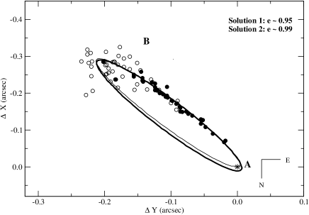
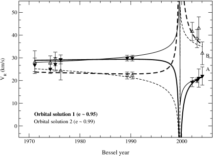
Although micrometric observations of DG Leo exist since 1935 (Kuiper 1935), no orbit is known yet. Fekel & Bopp (1977) roughly estimated an orbital period of 180 $\pm$ 50 yrs based on calibrations of spectral type versus mass and absolute magnitude. Notice that in their study a parallax of 0.007″was adopted which is in full concordance with the Hipparcos parallax (6.34 $\pm$ 0.94 mas). In order to derive the orbital parameters, we requested all the observations of DG Leo AB from the Washington Double Star Observations Catalog (Mason et al. 2001) and obtained 44 micrometric and 38 speckle-interferometric measurements (see Table 5). We further received one unpublished speckle observation (Hartkopf, W., 2004, private comm.). Since 1997 the systematic observations were discontinued owing to the difficulty of access to sufficiently large telescopes for this type of object. Unfortunately, the astrometric data in themselves are insufficient to compute a reliable visual orbit, as practically no change in position angle was detected during a time interval of more than 40 years. To complete the data we therefore included the components’ radial velocities (see Table 4) for a combined astrometric–spectroscopic orbit analysis. Use was made of the software package developed by Pourbaix (1998). It is based on the principles of simulated annealing (SA, Metropolis et al. 1953) for the global exploration and minimization in the parameter space followed by a local least-squares minimization (following the scheme of Broyden-Fletcher-Goldstrab-Shanno). Table 6 lists the stable and well-defined orbital parameters corresponding to one of the best solutions in the sense of least-squared residuals after 1500 iterations with SA and exploring the period range 70–200 years. Fig. 3 illustrates this orbit, both for the visual (upper panel) and the spectroscopic (lower panel) datasets (cf. Table 4). The accuracy and the confidence level of this solution are further discussed in Sect. 8.2.

Table 4: Radial velocities of components A and B. FB77: Fekel & Bopp (1977); RS91: Rosvick & Scarfe (1991); EB2002: ELODIE observations made by Oblak (2002); PN2003: ELODIE observations performed by North (2003); PM2004: ELODIE observations obtained by Mathias (2004).

JD	Va	Vb	Ref.
	(km s-1)	(km s-1)
2440995.9042	26.9 $\pm$ 3	28.1 $\pm$ 5	FB77
2442113.9789	25.1 $\pm$ 2	27.9 $\pm$ 4	FB77
2442470.8851	27.2 $\pm$ 3	29.5 $\pm$ 3	FB77
2442856.8086	29.3 $\pm$ 2	24.3 $\pm$ 4	FB77
2447815.7210	29.9 $\pm$ 2	22.2 $\pm$ 2	RS91
2452300.6250	19.3 $\pm$ 2	41.6 $\pm$ 4	EB2002
2452649.0512	20.1 $\pm$ 1	38.5 $\pm$ 4	this work
2452771.3452	21.1 $\pm$ 4	43.0 $\pm$ 5	PN2003
2453026.6498	22.0 $\pm$ 4	32.0 $\pm$ 5	PM2004

Table 5: Sample of micrometric ($\theta$, $\rho$) and speckle (x, y). The data are followed by the residuals (O$-$C). A full version of this table is available at the CDS.

micrometric data
Epoch	$\theta$(°)	(O$-$C)$\theta$	$\rho$(″)	(O$-$C)$\rho$
1935.4400	218.360	$+$3.548	0.335	$-$0.005
1936.8700	218.118	$-$5.715	0.339	$-$0.019
1937.1100	218.078	$+$11.524	0.339	$-$0.039
1937.2800	218.049	$+$8.852	0.340	$-$0.040
1938.1600	217.904	$+$0.195	0.342	$-$0.042
…
speckle data
Epoch	x(”)	(O$-$C)x	y(”)	(O$-$C)y
1940.1200	$-$0.274	$-$0.010	$-$0.211	$+$0.008
1976.8606	$-$0.249	$-$0.001	$-$0.152	$-$0.004
1977.1802	$-$0.247	$+$0.011	$-$0.151	$-$0.032
1977.3331	$-$0.247	$+$0.002	$-$0.150	$-$0.006
1978.3161	$-$0.242	$-$0.015	$-$0.146	$+$0.001
…

Figure 3: Upper panel: Observations and computed relative visual orbits: the best solution is represented by the thick solid curve while the other represents an orbit with an eccentricity very close to 1. The micrometric and speckle data obtained from 1935 to 1997 are represented by open and filled circles respectively. Lower panel: Observed (comp A: open triangles – comp B: filled triangles) and predicted (comp A: solid curve and comp B: dashes) radial-velocity variations for the two solutions (thick and thin curves) shown in the upper panel (see discussion in Sect. 8.2).

Table 6: Values and standard deviations of the constrained parameters of the combined astrometric-spectroscopic orbital solution of DG Leo AB.

Orbital parameter	Value			Std. dev.
$a$ (″)	0	.	191	0	.	015
$i$ (°)	117	.		13	.
$\omega$ (°)	341	.		13	.
$\Omega$ (°)	27	.	2	3	.	0
$e$	0	.	946	0	.	043
$P$ (yr)	102	.	3	9	.	5
$T$ (Besselian year)	1999	.	59	0	.	41
$V_{0}$ (km s-1)	+26	.	97	0	.	49
$\kappa=\frac{M_{\rm B}}{M_{\rm A}+M_{\rm B}}$	0	.	374	0	.	046

6 Atmospheric fundamental parameters

The disentangled component spectra provided by korel allow the use of well known techniques of spectral analysis that lead to the determination of physical quantities (i.e.: T_eff, log g and $V\!\sin i$) accurately describing the stellar atmospheres. For DG Leo’s components, these atmospheric fundamental parameters were derived in three consecutive steps which are chronologically described in the following subsections and the results of which are listed in Table 7.

6.1 Projected rotation velocity

A Fourier analysis of several unblended line profiles was used to determine the projected rotation velocity (V sin i). The adopted procedure that uses a FFT fortran subroutine provided by Gray (1992) is similar to the one described by Carroll (1933) and largely applied for example by Royer et al. (2002). It is based on the location of the first minimum of the Fourier transform that varies as the inverse of V sin i. Twelve isolated spectral lines were therefore chosen in the disentangled spectra (see Sect. 4). The projected rotation velocities thus derived are given in Table 7. The listed error is equal to the root mean square of the measurements made on each of the 12 unblended lines. Our $V\!\sin i$ measurements confirm the general trend that is observed when the widths of the cross-correlation functions (Fig. 1) for each component are compared to each other: DG Leo Aa is apparently rotating faster than DG Leo Ab. This unexpected result is discussed in Sect. 8.5.

Figure 4: Fitting of the observed hydrogen line profiles (dots) with theoretical spectra (line).

6.2 Effective temperature

In the atmospheres of mid- to late-A-type stars, hydrogen exists mostly in a neutral form. Hydrogen lines are therefore rather insensitive to surface gravity and can be used to derive the effective temperature (see for example:  Smalley & Dworetsky 1993). Consequently, we estimated the effective temperature of DG Leo’s components by fitting the individual H$\alpha$ and H$\gamma$ lines with theoretical line profiles (Fig. 4). Fully line-blanketed model atmospheres were computed in LTE with atlas 9 (Kurucz 1993a) corrected to account for the comments made by Castelli et al. (1997). From these models, a flux grid was obtained by use of the synspec computer code (Hubeny & Lanz 1995, see references therein) enabling the IRSCT and IOPHMI opacity flags, respectively, to account for the Rayleigh scattering and for the H^- ions. A least-squares method and the minuit minimization package of CERN were finally used to fit the observed line profiles. During the procedure, the surface gravity was kept fixed to 4. (cgs) for all three components. Error bars were computed from the largest deviation obtained by performing the fit several times and assuming different start values for the effective temperature.

6.3 Surface gravity

Because in late-A-type stars the hydrogen lines are insensitive to a change in surface gravity, we followed the same procedure as used by North et al. (1997) and Erspamer & North (2003) for stars within a distance of 150 pc to derive the surface gravity of the components. The luminosity was calculated from the hipparcos parallax of the triple star and the components’ V magnitudes (see Table 3). The bolometric correction was adopted from Flower (1996). Making use of the bolometric magnitude and the previously derived effective temperature, we then obtained the mass and the radius of each component through interpolation in the theoretical evolutionary tracks of Schaller et al. (1992) (for Z=0.001 and 0.020). In this way the surface gravities of the components were found to be much alike: the values are listed in Table 7 together with the interpolated masses (M_HR) and radii (R_HR). Their accuracy was estimated from the errors affecting the hipparcos parallax ($\frac{\sigma_{\pi}}{\pi}$=15%) and the effective temperature.

Table 7: Derived fundamental parameters

Star	Aa			Ab			B
Teff (K)	7470	$\pm$	220	7390	$\pm$	220	7590	$\pm$	220
log$~{}g$	3.8	$\pm$	0.14	3.8	$\pm$	0.14	3.8	$\pm$	0.12
V sin i  ($\rm{km~{}s^{-1}}$)	42	$\pm$	2	28	$\pm$	2	31	$\pm$	3
$\xi_{\rm{turb}}$ ($\rm{km~{}s^{-1}}$)	2.3	$\pm$	0.5	2.3	$\pm$	0.5	2.5	$\pm$	0.5
MHR (M⊙)	2.0	$\pm$	0.2	2.0	$\pm$	0.2	2.1	$\pm$	0.2
RHR (R⊙)	2.96	$\pm$	0.20	2.94	$\pm$	0.20	2.99	$\pm$	0.20

7 Abundance analysis

The disentangled spectra were used to estimate the components’ atmospheric chemical composition. We therefore systematically applied korel, order by order and from 4900 Å to 6100 Å, keeping the orbital parameters and luminosity ratios fixed to the values in Table 3 and Sect. 5.1. The abundance determination was then carried out by fitting theoretical line profiles to the observed components’ spectra (see Fig. 6).

7.1 Atomic data

Oscillator strengths, energy levels and damping parameters (including Stark, van der Waals and natural broadening) used during the fitting procedure were basically those compiled in the VALD-2 database (Kupka et al. 1999) updated by Erspamer & North (2002). For elements having atomic numbers greater than 30, the line list was completed by atomic data extracted from Kurucz CD-ROM N23 (Kurucz 1993b) and from the NIST Atomic Spectra Database (see the gfVIS.dat file created by Hubeny & Lanz 2003). Sc ii and Mn ii were treated with oscillator strengths proposed by Nissen et al. (2000).

7.2 Chemical composition

Figure 5: The abundance patterns we observed for the components of DG Leo are compared to those determined in the Sun (Grevesse & Sauval 1998) and in the Am star 32 Aqr (Kocer et al. 1993).

The microturbulent velocity was supposed to be constant with optical depth. It was derived simultaneously with the iron abundance by fitting the observations, from 4950 Å to 6100 Å, with theoretical spectra. Except for iron, during this procedure the chemical composition was kept fixed at the solar values. The resulting microturbulent velocities, $\xi_{\rm{turb}}$, are given in Table 7 and were further used to derive the abundances of the other atomic species.

A description of the model atmospheres and of the computer code we used can be found in Sect. 6.2. For the same line lists and model atmospheres, there is generally a good agreement between the synthetic spectra provided by synspec46 and those computed by other programs such as spectrum which was written by R.O. Gray (e.g.: Gray & Corbally 1994). However, Sc ii line profiles were systematically much stronger in synspec’s spectra, providing scandium abundances one order of magnitude smaller than expected for our reference star. The use of Kurucz’s pfsaha subroutine, to compute the partition functions of scandium, definitely resolved this incoherence. It is worth noting that this problem does not occur with the older versions of synspec.

Table 8: Components’ chemical compositions relative to hydrogen

	DG Leo			n	Sun
	$\epsilon$(Aa)	$\epsilon$(Ab)	$\epsilon$(B)
Na	$-$5.47 $\pm$ 0.13	$-$5.52 $\pm$ 0.13	$-$5.63 $\pm$ 0.13	1	$-$5.67
Mg	$-$4.42 $\pm$ 0.17	$-$4.64 $\pm$ 0.17	$-$4.27 $\pm$ 0.17	2	$-$4.42
Si	$-$4.48 $\pm$ 0.11	$-$4.51 $\pm$ 0.06	$-$4.48 $\pm$ 0.05	3	$-$4.45
Ca	$-$5.65 $\pm$ 0.15	$-$5.84 $\pm$ 0.17	$-$5.57 $\pm$ 0.13	4	$-$5.64
Sc	$-$9.29 $\pm$ 0.16	$-$9.35 $\pm$ 0.16	$-$8.87 $\pm$ 0.16	2	$-$8.83
Ti	$-$6.74 $\pm$ 0.09	$-$6.87 $\pm$ 0.09	$-$6.80 $\pm$ 0.08	5	$-$6.82
Cr	$-$6.03 $\pm$ 0.12	$-$6.12 $\pm$ 0.12	$-$6.31 $\pm$ 0.12	8	$-$6.33
Mn	$-$6.66 $\pm$ 0.13	$-$6.60 $\pm$ 0.13		2	$-$6.61
Fe	$-$4.32 $\pm$ 0.07	$-$4.33 $\pm$ 0.08	$-$4.54 $\pm$ 0.08	30	$-$4.50
Ni	$-$5.40 $\pm$ 0.09	$-$5.50 $\pm$ 0.11	$-$5.63 $\pm$ 0.11	7	$-$5.75
Y	$-$8.78 $\pm$ 0.14	$-$8.67 $\pm$ 0.14	$-$9.74 $\pm$ 0.16	5	$-$9.78
Zr	$-$8.49 $\pm$ 0.16	$-$8.39 $\pm$ 0.16		1	$-$9.39
Nd	$-$9.50 $\pm$ 0.26	$-$9.48 $\pm$ 0.26		4	$-$10.50

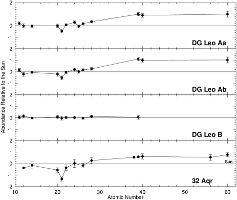
The final results of the chemical analysis are summarized in Table 8 and in Fig. 5. An example of the agreement obtained between the fitted synthetic spectra and the disentangled ones is shown in Fig. 6. Logarithmic abundance values are given relatively to hydrogen for the Sun (Col. 6) as well as for each component of DG Leo (Col. 2, 3 and 4). Solar abundances were taken from Grevesse & Sauval (1998). The number of transitions considered to derive the atmospheric chemical composition of DG Leo’s components is noted in Col. 5. Abundance error bars, $\Delta\epsilon$, were computed in the framework of non–correlated error sources with the following relation:

$$\sigma^{2}~{}=~{}{{\sigma^{2}_{\rm{scat}}}\over{n-1}}~{}+~{}\Delta\epsilon{\rm{(Teff)}}^{2}~{}+~{}\Delta\epsilon{\rm{(log~{}g)}}^{2}~{}+~{}\Delta\epsilon{\rm(\xi_{\rm{turb}})}^{2}$$ (1)

where n is the number of lines that we used and where $\sigma_{\rm{scat}}$, $\Delta\epsilon{\rm{(Teff)}}$, $\Delta\epsilon{\rm{(log~{}g)}}$ and $\Delta\epsilon{\rm(\xi_{\rm{turb}})}$ are the errors related respectively to the r.m.s. scatter of the derived abundance, to the effective temperature, surface gravity and microturbulent velocity accuracy. The uncertainties $\Delta\epsilon$ on the abundance introduced by the fundamental parameters are given in Table 9. They were computed relatively to a reference atmosphere model defined by the following fundamental parameters: T_eff = 7500 K, log g = 4.0, $\xi_{\rm{turb}}$ = 2.5 km s^-1 and solar chemical composition. When only one line is available to determine the abundance, the computation of $\sigma_{\rm{scat}}$ is based on the oscillator strength’s relative error (fixed at 25% when not found in the NIST database).

Figure 6: Comparison between the vertically shifted normalized component spectra (thick line) and the fitted synthetic spectra resulting from the chemical abundance analysis (thin line). Identifications indicate the transitions contributing the most to the spectral lines.

Table 9: Abundance deviations ($\Delta\epsilon$) caused by the upper and lower limits of T_eff, log g and microturbulent velocity ($\xi_{\rm{turb}}$).

Elem.	$\Delta\epsilon{\rm{(Teff)}}$	$\Delta\epsilon{\rm{(log~{}g)}}$	$\Delta\epsilon{\rm(\xi_{\rm{turb}})}$
Na	0.03	0.02	0.05
Mg	0.10	0.04	0.07
Si	0.02	0.02	0.00
Ca	0.03	0.01	0.06
Sc	0.01	0.06	0.13
Ti	0.02	0.05	0.05
Cr	0.06	0.01	0.03
Mn	0.05	0.00	0.04
Fe	0.01	0.00	0.06
Ni	0.02	0.03	0.05
Y	0.02	0.05	0.09
Zr	0.02	0.11	0.05
Nd	0.08	0.07	0.05

8 Discussion

8.1 Spectroscopic orbit of the close binary Aab

The parameters we derived for the spectroscopic binary are in good agreement with the previously published values (Fekel & Bopp 1977; Rosvick & Scarfe 1991). From the spectroscopic orbital parameters listed in Sect 5.1, one may further derive:

$$(\rm{a_{Aa}+a_{Ab}})\sin i_{\rm A} = \rm{16.5}\pm\rm{0.02~{}R_{\odot}}$$ (2)

$$\rm{M_{Aa}}\sin^{3}i_{\rm A} = \rm{1.760}\pm\rm{0.007~{}M_{\odot}}$$ (3)

$$= \rm{M_{Ab}}\sin^{3}i_{\rm A}$$ (4)

where $i_{\rm A}$ stands for the inclination of the close binary and where we introduced the values of K, q, P and e as well as their associated error bars. Since no eclipses were observed (Lampens et al. 2005), the derived orbital parameters constrain the orbital inclination angle which will depend on the stellar radius and thus on the surface gravity. From the condition $\rm{R_{Aa}}+\rm{R_{Ab}}<(\rm{a_{Aa}+a_{Ab}})\cos i$ (no eclipses), we have that:

$\tan~{}i_{\rm A}$

$<$

${(\rm{a_{Aa}+a_{Ab}})~{}\sin~{}i_{\rm A}}\over{R_{Aa}+R_{Ab}}$

For $\rm{R_{Aa}}=\rm{R_{Ab}}=R$ and if we use $\rm{R^{\rm{-1}}}\propto(g/M)^{1/2}$ in relations (2) and (3), we obtain:

$$\sin i_{\rm A}\cos^{2}i_{\rm A} > \frac{{\rm M}\sin^{3}i_{\rm A}/\rm{M_{\odot}}}{\left({\rm{(a_{Aa}+a_{Ab})}}/{2}\right)^{2}}\frac{\rm g_{\odot}}{\rm g}$$ (5)

$$> 0.02586~{}\frac{\rm g_{\odot}}{\rm g}$$ (6)

Numerically for $\log g=3.8\pm 0.14$ (see Table 7), we find:

$$i_{\rm A}<69^{\rm o}_{\rm.}8^{\rm+3.2}_{\rm-4.2}$$ (7)

implying an upper limit for the orbital inclination of 73^o from the absence of eclipses. Comparing the stellar masses derived from the evolution tracks (see M_HR in Table 7), it is clear that the orbital inclination cannot be much lower, as the lower mass limit deduced from (7) and (4) gives:

$$\rm{M_{Aa}}=\rm{M_{Ab}} > 2.1^{+0.2}_{-0.1}~{}\rm{M_{\odot}}.$$ (8)

8.2 Astrometric–spectroscopic orbit of the wide binary AB

Recent and old astrometric data were combined with radial velocities obtained at an epoch close to periastron passage. Using different starting points corresponding to the 100 lowest values of the objective function found with SA, we ended up with the solution proposed in Sect. 5.2 in 80% of the cases after a fine tuning of the minimization process. In only 3% of the cases, SA converged successfully to solutions with some parameter out of the 1.5-$\sigma$ uncertainties given in Table 6. Although the residuals are realistic given the measurement errors, the orbit is not yet definitive. Some parameters remain unconstrained because we miss radial velocities near periastron in a very eccentric orbit. At present, we conclude that:

• the orbital period is notably shorter than previously estimated by Fekel & Bopp (1977), with a most probable value close to 100 years (and an uncertainty of 10%);

• the orbit is definitely very eccentric, but unfortunately we do not have radial velocities near periastron. Any spectra taken in the interval 1998–2002 would be of immense value if existing;

• the fractional mass is constrained reasonably well with a most probable value $\kappa$ = 0.37, and consistent with the value derived from the fundamental atmospheric parameters ($\kappa$ = 0.34 $\pm$ 0.07). The constraint on the orbital $\kappa$ already induces a useful lower limit to the mass of component B relative to each of the equal-mass components of A:

  $$\frac{\rm{M_{B}}}{\rm{M_{A_{a}}}} > 1.19^{-0.21}_{+0.26}.$$ (9)

  In other words, component B is very probably at least as massive as each of the close binary components;

• the other constrained parameters (Table 6) include the orbital inclination (range 110–130 degrees) and those related to the astrometric data;

• ambiguity remains with several parameters related to the unconstrained radial-velocity amplitude (see the two different solutions shown in Fig. 3). As a consequence, we do not know the true semi-axis major (in km s^-1), which would provide a dynamical parallax and absolute masses.

Hence, we can use the mass of component A obtained from the close spectroscopic orbit. From Table 7 and eq. 8, we have $M_{A}=4.2\pm 0.2~{}M_{\sun}$. Then the data of Table 6, together with standard–error propagation laws, lead to:

$$\rm{M_{B}} = 2.5\pm 0.6~{}\rm{M_{\odot}}$$

$$\rm{K_{A}} = 12.3\pm 5.8~{}\rm{km~{}s}^{\rm{-1}}$$

$$\rm{K_{B}} = 20.6\pm 8.7~{}\rm{km~{}s}^{\rm{-1}}$$

$$\rm{a}=\rm{a_{A}+a_{B}} = 41.2\pm 5.8~{}\rm{AU}$$

$$\pi = 4.6\pm 1.0~{}\rm{mas},$$

where the dynamical parallax is consistent with the Hipparcos parallax at the 1.3–$\sigma$ level.

A next step would be to repeat the SA procedure limiting the exploration of the parameter space to realistic values of $\rm{M_{A}}$. However, significant progress in the direct determination of the individual masses with a sufficiently high accuracy could be achieved, either by including possibly existing radial velocities near periastron passage – we therefore invite anyone who might have spectra or radial velocities of DG Leo during the interval 1998–2002 (see Fig. 3) to contact us – or by gathering new speckle-interferometric observations in the following years.

8.3 Ca abundance and luminosity ratios

As noted in Sect. 4, the luminosity ratios of the three components were derived under the assumption that their Ca ii K line-depths are saturated and identical. To test the validity range of that assumption, we compare in Fig. 7 the theoretical spectra of all three components of DG Leo from 3920 to 3950 Å. Owing to the close values of the fundamental parameters and to the fact that the calcium underabundance observed in the close binary components is smaller than 0.20 dex, the line depths are very similar. As a matter of fact, the slightly smaller depth in the spectrum of the faster rotating component Aa might have introduced a flux zero–point error smaller than 1.5 percent, which does not significantly affect the abundance analysis.

Figure 7: Computed Ca ii K line-profile for all three components of DG Leo.

Figure 8: The spectrum of the chemically normal star HD 33959 (top) and the ratio of the Am and DG Leo spectra (components Ab and B only) to the top one are plotted.

8.4 Comparison with reference stars

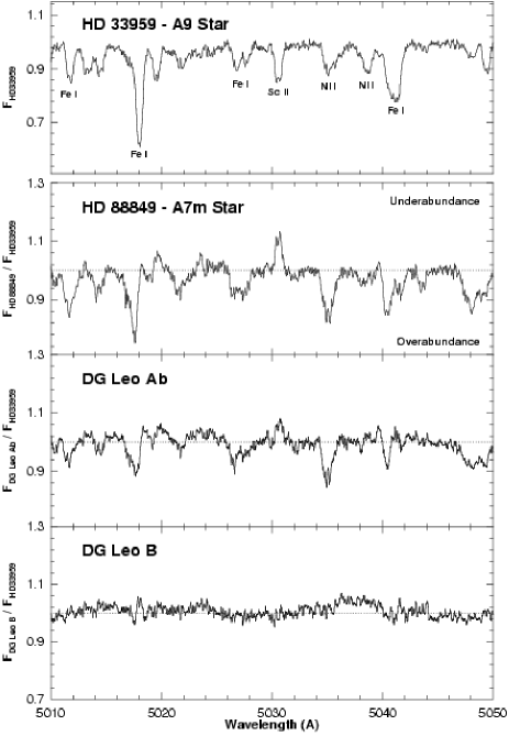
If we discount the larger effects of Doppler broadening for DG Leo Aa, both components of the close binary have very similar spectra. Their nature is however different from that of component B and their iron-peak lines are generally significantly stronger. To visualize the general trend that can be noted in the chemical abundances we derived, their respective spectra have been compared to the spectra of the A9 star HD 33959 (14 Aur) and the metal-line A7m star HD 88849 (HR 4021) found in The Elodie Archive at OHP. These stars are similar to DG Leo’s components in spectral type and projected rotation velocity, but different in chemical composition. To make this more obvious, the spectra of HD 88849 and those of the Ab and B components were divided by the reference spectrum of HD 33959 and reported in Fig. 8. According to this comparison, DG Leo B is found to have almost the same chemical composition and fundamental parameters as the reference star which is known to be chemically normal (Hui-Bon-Hoa 2000). For their part, the A components present typical Am-type peculiarities (e.g.: scandium deficiency and enhanced iron-peak elements) but somewhat weaker than those observed in HD 88849. From a quantitative point of view, our abundance analysis clearly shows that in the A components’ atmospheres, iron-peak elements are overabundant by up to 0.2 dex relatively to the Sun and by up to 1.0 dex for the heavier elements (Y, Zr, Nd). The overabundances are therefore of the same order of magnitude as is observed in other typical Am stars such as 32 Aqr (HD 209625, see Fig. 5). Deficient species, especially calcium, are less extremely underabundant in the close binary components of DG Leo.

Figure 9: The spectra of DG Leo Aa (line) and DG Leo Ab (dots) are compared. The spectrum of the latter component was convolved with a Gaussian function in order to increase artificially its projected rotation velocity.

8.5 The close binary components Aa and Ab

Spin–orbit synchronization is generally expected to occur 100 times faster than orbital circularization (Zahn 1977). Stars in an already circularized orbit are therefore expected to be synchronized and to have similar projected rotation velocities. As mentioned earlier, this is obviously not the case for the close binary of DG Leo. We note indeed (Sect. 6.1) a significant disagreement between the $V\!\sin i$ values of the two components. The predicted synchronization velocity V_synch=36$\pm$6 km s^-1 lies in between the measured values. Therefore, we cannot exclude that one of the components would be synchronized. This certainly merits further attention.

Components of multiple systems such as DG Leo usually originate from the same protostellar environment. Their similarity or difference in chemical surface composition therefore relates directly to their individual/uncoupled evolution after formation (stellar evolution, rotation, diffusion), and the possible influence of a close companion. It is known from Sect. 6 that the Aa and Ab components have similar fundamental parameters. As can be noted from Table 8 and from Fig. 5, they further have very similar abundance patterns. Both components are Am stars showing the same magnitude of overabundance for the iron-peak elements as well as for the heavier ones. The underabundances are mild compared to many classical Am stars. A differential comparison of the disentangled spectra of Aa and Ab (Fig. 9) gives evidence for a marginally higher Ca abundance in Aa. This fact remains unnoticed from Table 8 because the uncertainties given on the abundances include the uncertainty on the fundamental atmospheric parameters at an absolute level. When comparing Aa and Ab, only the relative errors in $\Delta$T_eff, $\Delta$log g and $\Delta\xi_{\rm{turb}}$ are relevant.

Classical diffusion models (Alecian 1996) generally show that calcium and scandium are leaving the atmosphere after a while. Observations (North 1993; Kunzli & North 1998) and numerical simulations (Alecian 1996) predict a short phase of calcium overabundance at the beginning of the main sequence followed by a calcium abundance decrease. In this sense, abundances are suspected to be very sensitive to mass loss, rotation and age which may explain the somewhat different behaviour regarding diffusion observed in the components Aa and Ab of DG Leo.

8.6 Spectral line variability

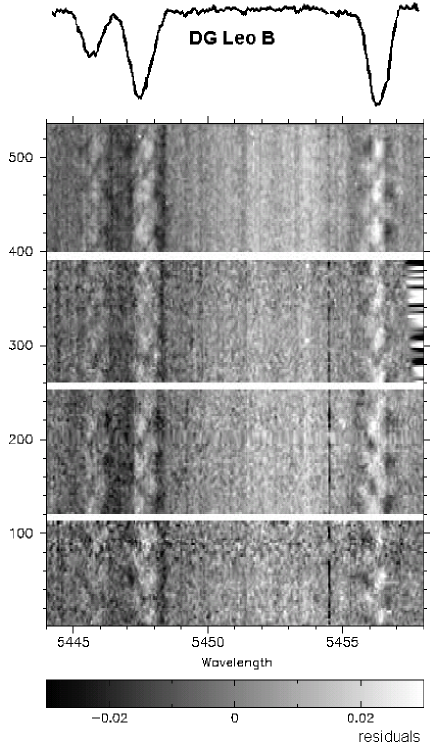
The residuals of korel clearly indicate that the spectroscopic variations due to pulsations are centred on the spectrum of component B (Fig. 10). The pattern of these variations is reproduced with a regularity of about 2 hours which agrees with the results from the photometry (Lampens et al. 2005). A detailed study of the line variability awaits the analysis of the photometry as both sources should be combined in a periodicity analysis (our time base for spectroscopy is very short) to enhance the probability of identifying the pulsation modes. However, we note already the multi-periodic character of the line variability from the lack of exact repetition of the variability patterns in different nights.

Despite this line variability, we further notice that the time-averaged spectrum of each component of DG Leo is fully consistent with the combined observed spectra and no numerical artifacts were detected. The use of korel to disentangle the component spectra from the high-resolution data may thus be considered as highly successful in this specific case.

Figure 10: The residuals provided by korel are plotted in a gray scaled figure for 4 consecutive nights (January 11 – 15, 2003). Each variation is centred on the spectrum of component B and repeats with a period of about 2 hours.

9 Conclusions

The Fourier Transform spectral disentangling technique developed by Hadrava (1995) was successfully applied to the study of the pulsating triple system DG Leo. It allowed to confirm the previously derived parameters of the spectroscopic orbit by Fekel & Bopp (1977) and to increase the accuracy. Combining astrometric measurements with our new radial-velocity measurements, we were further able to compute for the first time the relative orbit of the visual system AB. However, we stress the fact that speckle and RV measurements at periastron would be invaluable. We would like therefore to be informed about such data, if existing, as these measurements should greatly increase the precision of the present solution and it could further enable the determination of the stellar masses of all 3 components in an independent way.

A detailed chemical analysis was performed on the disentangled spectra of the components with the Kurucz LTE model atmospheres combined with the synspec computer codes. All three components appear to have the same fundamental parameters (effective temperature and surface gravity) but DG Leo B was found to have a solar-like chemical composition, while the two components belonging to the close spectroscopic binary show an abundance pattern typical of Am stars. A different level of underabundance for scandium and more strongly for calcium is noted between the two close components (Aa and Ab). These differences probably reflect the sensitivity of the diffusion processes to issues such as rotation, mass loss and evolution. We further noticed that, while the spectroscopic orbit is circularized, the apparent rotation of both A components is not yet synchronized with the orbital motion. DG Leo is therefore a very interesting clue for understanding issues such as rotation synchronization and orbital circularization.

Our high–time–resolution spectroscopic data confirm the existence of line–profile variations (LPVs) caused by pulsation in component B with time scales very close to those recently detected by photometric studies (Lampens et al. 2005). The analysis and the mode identification of these LPVs will be combined with the multicolour photometric observations, with the goal to provide a better understanding of the non-trivial link existing between chemical composition, multiplicity and pulsation.

References

- Alecian (1996) Alecian, G. 1996, A&A, 310, 872
- Baranne et al. (1996) Baranne, A., Queloz, D., Mayor, M., et al. 1996, A&AS, 119, 373
- Breger (2000) Breger, M. 2000, in ASP Conf. Ser. 210: Delta Scuti and Related Stars, ed. M. Breger & M. H. Montgomery, 3
- Budaj (1996) Budaj, J. 1996, A&A, 313, 523
- Budaj (1997) Budaj, J. 1997, A&A, 326, 655
- Carroll (1933) Carroll, J. A. 1933, MNRAS, 93, 478
- Castelli et al. (1997) Castelli, F., Gratton, R. G., & Kurucz, R. L. 1997, A&A, 318, 841
- Cowley (1976) Cowley, A. P. 1976, PASP, 88, 95
- Cowley & Bidelman (1979) Cowley, A. P. & Bidelman, W. P. 1979, PASP, 91, 83
- Danziger & Dickens (1967) Danziger, I. J. & Dickens, R. J. 1967, ApJ, 149, 55
- De Cat et al. (2004) De Cat, P., De Ridder, J., Hensberge, H., & Ilijić, S. 2004, in ASP Conf. Ser. 318: Spectroscopically and spatially resolving the components of close binary stars, ed. Hilditch et al., 338
- Eggen (1979) Eggen, O. J. 1979, ApJS, 41, 413
- Elliott (1974) Elliott, J. E. 1974, AJ, 79, 1082
- Erspamer & North (2002) Erspamer, D. & North, P. 2002, A&A, 383, 227
- Erspamer & North (2003) Erspamer, D. & North, P. 2003, A&A, 398, 1121
- ESA (1997) ESA. 1997, in The Hipparcos and Tycho Catalogues ESA–SP 1200 (Vol. 1)
- Faraggiana & Gerbaldi (2003) Faraggiana, R. & Gerbaldi, M. 2003, A&A, 398, 697
- Fekel & Bopp (1977) Fekel, F. C. & Bopp, B. W. 1977, PASP, 89, 216
- Flower (1996) Flower, P. J. 1996, ApJ, 469, 355
- Gerbaldi et al. (2003) Gerbaldi, M., Faraggiana, R., & Lai, O. 2003, A&A, 412, 447
- Gray (1992) Gray, D. F. 1992, The observation and analysis of stellar photospheres (Cambridge Astrophysics Series, Cambridge: Cambridge University Press, 2nd ed., ISBN 0521403200.)
- Gray & Corbally (1994) Gray, R. O. & Corbally, C. J. 1994, AJ, 107, 742
- Grevesse & Sauval (1998) Grevesse, N. & Sauval, A. J. 1998, Space Science Reviews, 85, 161
- Griffin (2002) Griffin, R. E. 2002, AJ, 123, 988
- Hadrava (1995) Hadrava, P. 1995, A&AS, 114, 393
- Harmanec et al. (2004) Harmanec, P., Uytterhoeven, K., & Aerts, C. 2004, A&A, 422, 1013
- Hensberge et al. (2000) Hensberge, H., Pavlovski, K., & Verschueren, W. 2000, A&A, 358, 553
- Hoffleit & Jaschek (1982) Hoffleit, D. & Jaschek, C. 1982, The Bright Star Catalogue (New Haven: Yale University Observatory (4th edition))
- Hubeny & Lanz (1995) Hubeny, I. & Lanz, T. 1995, ApJ, 439, 875
- Hubeny & Lanz (2003) Hubeny, I. & Lanz, T. 2003, http://tlusty.gsfc.nasa.gov/
- Hui-Bon-Hoa (2000) Hui-Bon-Hoa, A. 2000, A&AS, 144, 203
- Ilijić (2004) Ilijić, S. 2004, in ASP Conf. Ser. 318: Spectroscopically and spatially resolving the components of close binary stars, ed. Hilditch et al., 107
- Ilijić et al. (2004) Ilijić, S., Hensberge, H., Pavlovski, K., & Freyhammer, L. 2004, in ASP Conf. Ser. 318: Spectroscopically and spatially resolving the components of close binary stars, ed. Hilditch et al., 111
- Kocer et al. (1993) Kocer, D., Adelman, S. J., Bolcal, C., & Hill, G. 1993, in ASP Conf. Ser. 44: IAU Colloq. 138: Peculiar versus Normal Phenomena in A-type and Related Stars, ed. M. M. Dworetsky, F. Castelli & R. Faraggiana, 213
- Kuiper (1935) Kuiper, G. P. 1935, PASP, 47, 230
- Kunzli & North (1998) Kunzli, M. & North, P. 1998, A&A, 330, 651
- Kupka et al. (1999) Kupka, F., Piskunov, N., Ryabchikova, T. A., Stempels, H. C., & Weiss, W. W. 1999, A&AS, 138, 119
- Kurtz (2000) Kurtz, D. W. 2000, in ASP Conf. Ser. 210: Delta Scuti and Related Stars, ed. M. Breger & M. H. Montgomery, 287
- Kurucz (1993a) Kurucz, R. L. 1993a, CD-ROM No.13. Cambridge, Mass.: Smithsonian Astrophysical Observatory.
- Kurucz (1993b) Kurucz, R. L. 1993b, CD-ROM No.23. Cambridge, Mass.: Smithsonian Astrophysical Observatory.
- Lampens et al. (2005) Lampens, P., Garrido, R., Parrao, L., et al. 2005, IAU 191 colloquium held in Merida (Mexico), Feb. 2003, eds. C. Allen & C. Scarfe, Rev. Mex. A.A., in press
- Mason et al. (2001) Mason, B. D., Wycoff, G. L., Hartkopf, W. I., Douglass, G. G., & Worley, C. E. 2001, AJ, 122, 3466
- Mathias (2004) Mathias, P. 2004, private communication
- Metropolis et al. (1953) Metropolis, N., Rosenbluth, A., Rosenbluth, M., Teller, A., & Teller, E. 1953, J. Chem. Phys., 21, 1087
- Nissen et al. (2000) Nissen, P. E., Chen, Y. Q., Schuster, W. J., & Zhao, G. 2000, A&A, 353, 722
- North (1993) North, P. 1993, in ASP Conf. Ser. 44: IAU Colloq. 138: Peculiar versus Normal Phenomena in A-type and Related Stars, ed. M.M. Dworetsky et al., 577
- North (2003) North, P. 2003, private communication
- North et al. (1997) North, P., Jaschek, C., & Egret, D. 1997, in ESA SP-402: Hipparcos - Venice ’97, 367
- Oblak (2002) Oblak, E. 2002, private communication
- Pourbaix (1998) Pourbaix, D. 1998, A&AS, 131, 377
- Rodríguez & Breger (2001) Rodríguez, E. & Breger, M. 2001, A&A, 366, 178
- Rosvick & Scarfe (1991) Rosvick, J. M. & Scarfe, C. D. 1991, PASP, 103, 628
- Royer et al. (2002) Royer, F., Gerbaldi, M., Faraggiana, R., & Gómez, A. E. 2002, A&A, 381, 105
- Schaller et al. (1992) Schaller, G., Schaerer, D., Meynet, G., & Maeder, A. 1992, A&AS, 96, 269
- Schwarzenberg-Czerny (1998) Schwarzenberg-Czerny, A. 1998, Baltic Astronomy, 7, 43
- Simon & Sturm (1994) Simon, K. P. & Sturm, E. 1994, A&A, 281, 286
- Smalley & Dworetsky (1993) Smalley, B. & Dworetsky, M. M. 1993, in ASP Conf. Ser. 44: IAU Colloq. 138: Peculiar versus Normal Phenomena in A-type and Related Stars, ed. M.M. Dworetsky et al., 182
- Sturm & Simon (1994) Sturm, E. & Simon, K. P. 1994, A&A, 282, 93
- Turcotte et al. (2000) Turcotte, S., Richer, J., Michaud, G., & Christensen-Dalsgaard, J. 2000, A&A, 360, 603
- Weiss & Paunzen (2000) Weiss, W. W. & Paunzen, E. 2000, in ASP Conf. Ser. 210: Delta Scuti and Related Stars, ed. M. Breger & M. H. Montgomery, 410
- Zahn (1977) Zahn, J.-P. 1977, A&A, 57, 383