Linear Accelerating Superluminal Motion Model

Abstract

Accelerating superluminal motions were detected recently by multi-epoch Very Long Baseline Interferometry (VLBI) observations. Here, a Linear Accelerating Superluminal Motion (LASM) model is proposed to interpret the observed phenomena. The model provides a direct and accurate way to estimate the viewing angle of a relativistic jet. It also predicts that both Doppler boosting and deboosting effects may take place in an accelerating forward jet. The LASM model is applied to the data of the quasar 3C 273, and the initial velocity, acceleration and viewing angle of its three components are derived through model fits. The variations of the viewing angle suggest that a supermassive black hole binary system may exist in the center of 3C273. The gap between the inner and outer jet in some radio loud AGNs my be explained in terms of Doppler deboosting effects when the components accelerate to ultra-relativistic speed.

1 Introduction

Superluminal motions were first detected by Very Long Baseline Interferometry (VLBI) in 1970s (Cohen et al., 1977). The observations carried out since then showed that such motions are quite common in blazars. Many models were proposed to explain the phenomenon, which were reviewed by Blandford et al. (1977). The relativistic jet model (Blandford & Königl, 1979) has become the de facto standard model to describe the superluminal motion.

From a simple physical consideration, acceleration is required to drive the subrelativistic material in the accretion disk up to the relativistic speed observed in the jets. Acceleration is also necessary to compensate the radiation losses in jets. There is increasing evidence that the central engine of acceleration in AGNs is a rotating supermassive black hole surrounded by a geometrically thin accretion disk, which gives rise to the formation of a pair of relativistic jets. The mechanism of acceleration may be due to the centrifugal and shear effects (Webb et al., 1994; Rieger & Mannheim, 2002). In recent years, multi-epoch VLBI monitoring indeed led to the discovery parsec-scale accelerating superluminal motion in the quasar 3C 273 (Krichbaum et al., 2001) and in other sources (Homan et al., 2001).

Currently, quadratic or cubic polynomials are usually employed to fit the accelerating superluminal motion curves (Krichbaum et al., 2001). Such mathematical fits, however, have no real physical meaning. Actually, a physical model is required to describe the observed phenomena. Here, we consider a simple model where a component is ejected out collinearly, with intrinsic constant acceleration $g$. Such acceleration may exist in rotating magnetized jets (Rieger & Mannheim, 2002), especially at the outsets of jets where the resistance of the intergalactic medium (IGM) can be neglected. Also, some theoretical work shows that the jets in pulsars indeed move outward with linear acceleration (Contopoulos & Kazanas, 2002). In the frame of special relativity, this model can interpret the accelerating superluminal motions, and we name it as a Linear Accelerating Superluminal Motion (LASM) model.

In this Letter, the LASM model will be introduced in detail. The basic kinematic equations of an accelerating relativistic component and their solutions are listed in Section 2. In Section 3, the proper motion of 3C 273 monitored with VLBI is model-fitted, and the viewing angle, initial velocity and acceleration of three components are estimated. Possible application of the LASM model, with emphasis on the estimates of the viewing angle and the evolution of the Doppler factor, are discussed in Section 4.

Throughout this Letter, we adopt a flat, accelerating cosmology with Hubble constant $H_{0}=71{\rm km\,s^{-1}\,Mpc^{-1}}$, $\Omega_{\Lambda}=0.73$ and $\Omega_{\rm m}=0.27$.

2 Linear Accelerating Kinematics

2.1 Basic Equations

We follow the relativistic jet model (Blandford & Königl, 1979). In this model, a component moves out along a collimated jet forming a viewing angle $\theta$ with the line of sight. The kinematics of this component can be described by the following equations

$$d\mu_{\rm ob} = \sin\theta\,\,dr$$ (1)

$$\beta = \frac{dr}{dt}$$ (2)

$$\frac{d\gamma\beta}{dt} = g$$ (3)

$$\frac{dt_{\rm ob}}{dt} = 1-\beta\cos\theta$$ (4)

$$\beta_{\rm app} = \frac{d\mu_{\rm ob}}{dt_{\rm ob}},$$ (5)

where $r$ is the displacement between the component and its origin, $\mu_{\rm ob}$ is the observed proper motion, $t$ and $t_{\rm ob}$ are the intrinsic time and the observer’s time respectively , $\beta$ and $\gamma=1/\sqrt{1-\beta^{2}}$ denote the component’s velocity (in units of the speed of light) and the Lorenz factor, $g$ is the acceleration, and $\beta_{\rm app}$ is the apparent velocity.

In order to interpret the accelerating superluminal motions observed by VLBI, the relationship between $\mu_{\rm ob}$ and $t_{\rm ob}$ should be derived based on the above equations. In case of linear acceleration where $\theta$ remains constant, the solution can be deduced through the solving routines of normal differential equations. It is worth noting that parametric equations, which describe the relationship between $\mu_{\rm ob}$ and $t_{\rm ob}$, are simpler to be derived than the “direct” solution of $\mu_{\rm ob}$ in terms of $t_{\rm ob}$.

2.2 Solutions

Assuming that $g$ is constant, parametric solutions of $\mu_{\rm ob}$ and $t_{\rm ob}$ can be derived. They are

$$\mu_{\rm ob} = \frac{\sin\theta}{k}\left[\sqrt{k^{2}t^{2}+2k\beta_{0}t+1}-1\right]$$ (6)

$$t_{\rm ob} = t-\frac{\cos\theta}{k}\left[\sqrt{k^{2}t^{2}+2k\beta_{0}t+1}-1\right],$$ (7)

where $k=g\sqrt{1-\beta_{0}^{2}}$, and $\beta_{0}$ is the initial velocity.

$\mu_{\rm ob}$ can also be written in terms of $t_{\rm ob}$ directly. If we eliminate $t$ in Equations 6 and 7, we obtain

$$\mu_{\rm ob}=\frac{1}{k\sin\theta}(\sqrt{T_{1}^{2}+T_{2}}-T_{1}),$$ (8)

where

$$T_{1} = 1-t_{\rm ob}k\cos\theta-\beta_{0}\cos\theta$$

$$T_{2} = (t_{\rm ob}^{2}k^{2}+2t_{\rm ob}k\beta_{0})\sin^{2}\theta.$$

The description of the other parameters of the jet components, such as apparent velocity $\beta_{\rm app}$ and Doppler boosting factor $D=\gamma^{-1}(1-\beta\cos\theta)^{-1}$, can also be derived from Equations 6, 7 and from the basic equations in Section 2.1. The corresponding formulas are

$$\beta_{\rm app} = \frac{\sin\theta(kt+\beta_{0})}{\sqrt{k^{2}t^{2}+2k\beta_{0}t+1}-\cos\theta(kt+\beta_{0})}$$ (9)

$$D = \frac{\sqrt{1-\beta_{0}^{2}}}{\sqrt{k^{2}t^{2}+2k\beta_{0}t+1}-\cos\theta(kt+\beta_{0})}.$$ (10)

Compared to the non-accelerating relativistic jet models, the accelerating model has some new interesting features. When $t$ is infinitesimal, the initial apparent velocity will be $\beta_{\rm ob}^{0}=\beta_{0}\sin\theta/(1-\beta_{0}\cos\theta)$. As $t$ increases, the apparent velocity will approach to its maximum value $\beta_{\rm ob}^{\rm max}=\cot(\theta/2)$ (Blandford & Königl, 1979). Concerning the Doppler factor $D$, it will first increase with $t$, and it will reach its maximum value $D^{\rm max}$, where $\beta=\cos\theta$ and $\gamma=D$. If the acceleration goes on, then $D$ will decrease, to values even lower than 1. Therefore, in an accelerating relativistic jet, both Doppler boosting and deboosting phenomena can be observed.

The LASM model can be applied to estimate the parameters of a relativistic jet. Equations 6 and 7 show that the shape of a proper motion curve is controlled by three parameters, i.e. $\beta_{0}$, $g$, and the viewing angle $\theta$. By comparing the model to the observed VLBI data, these parameters can be calculated. If multi frequency flux density data were combined with proper motion data, then the model fitting results would be more accurate.

Since the relativistic jets in AGNs probably exhibit different structures on different scales, we should carefully consider where the LASM model can be applied. On the large kpc scale, the jets usually have collinear structures. Although superluminal motions were detected by HST observations on such scale in M87 (Biretta et al., 1999), there are not enough data for a quantitive estimate of the jet parameters with LASM model. However, in this situation, the LASM model can still be used to qualitatively explain some interesting profiles of the jets (see Section 4.2). On the scale of tens of pc, the jets probably show ’wiggles’ or helical structures, and the LASM model cannot be used there. On the small scale, especially in the core regions of jets, where jet components usually move out collinearly, the LASM is applicable to assess the physical and geometrical parameters of jets.

3 Application to 3C273

3C 273 (J1229+0203) is a low optical polarization quasar (LPQ) with $z=0.158$ (Strauss et al., 1992). It was the first object to display apparent superluminal motion on parsec scales (Pearson et al., 1981). The radio structure of 3C 273 shows a well defined core-jet morphology from the mas scale up to the arc-second scale. The jet extends out to  20 arc-seconds, with the ridge line of emission showing a clear ’wiggle’ (Davis et al., 1985). VLBI imaging at frequencies from 5 to 100 GHz show that the ridge line of the jet is curved on a scale from 0.05 to 25 mas, oscillating around the main orientation of the jet (Baath et al., 1991; Krichbaum et al., 1990). Zensus et al. (1990) suggest that the discrepancy in the position angles of some of the components observed at different frequencies may reflect a spectral index gradient across the jet.

Since 1990, 3C 273 has been monitored with VLBI from 15 to 86 GHz. For the components with enough data points at small ($<$ 2mas) and large ($>$ 2mas) core separations, quadratic fits to the radial motion $r(t)$ describe the observations much better than linear fits (Krichbaum et al., 2001). This suggests that these components indeed have accelerating proper motions. Furthermore, in the inner region with radial distance less than 8 milli-arcsecond, these components seem to move outward collinearly. Therefore, the LASM model is suitable to describe the observed data, and estimate the viewing angles and accelerations the components via least square fits.

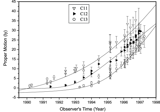
Figure 1: LASM model fitting results of the components C11, C12 and C13 in 3C 273.

The components C11, C12 and C13 in Krichbaum et al. (2001), which have enough good quality data, are chosen for the model fitting. The location of a component at the first epoch is set as the origin of the coordinate system, with $t_{\rm ob}=0$ and $\mu_{\rm ob}=0$. The original proper motion data and their fitted lines are shown in Figure 1. The corresponding parameters are listed in Table 1. Figure 2 shows the predicted evolution of the Doppler factors $D$ of the components.

Model fitting results show that the observed proper motion curves are sensitive to the viewing angle $\theta$ and to the initial velocity $\beta_{0}$. These two estimated parameters have relatively small errors. The acceleration factor $k$, however, has a larger error. The reason is that when a component accelerates to an ultra-relativistic velocity, its apparent velocity will remain almost constant, with $\beta_{\rm app}\approx\cot(\theta/2)$, thus lateral observed data will not dramatically contribute to the estimate of $k$. The $\chi^{2}$ values are lower than 1. This may due to the fact that the errors of the original proper motion data have been over-estimated. Table 1 and Figures 1 and 2, show that the Doppler factors of all the three components are decreasing in the last epoch.

4 Discussion

4.1 Viewing angle

The viewing angle plays an important role in the unification for radio-loud AGN. It is believed that all radio-loud AGNs have a similar physical structure: a supermassive black hole (probably spinning) located at their centre, whose gravitational potential energy is the ultimate origin of the AGN luminosity; an accretion disk surrounding the black hole, with relativistic jets emitted perpendicular to it; broad line and narrow line regions, and a dusty torus located at a larger distance from the innermost nucleus. The appearance of AGNs, however, depends so strongly on orientation that our current classification schemes are dominated by random pointing directions instead of more grounded physical properties. Thus, to understand the intrinsic mechanism of the AGNs, beaming effects induced by the viewing angle should be removed (Urry & Padovani, 1995).

Besides the apparent velocity measured by VLBI, other observational properties are needed to estimate the viewing angle. The apparent velocity $\beta_{\rm app}=\beta\sin\theta/(1-\beta\cos\theta)$ depends both on $\theta$ and $\beta$, so $\theta$ cannot be derived only from $\beta_{\rm app}$. If both apparent velocity $\beta_{\rm app}$ and Doppler boosting factor $D$ are known, then the viewing angle can be calculated (Ghisellini et al., 1993). $\beta_{\rm app}$ can be directly observed by VLBI. Currently, there are three ways to estimate $D$. The first one is based on synchrotron self-Compton (SSC) model (Marscher, 1987). The second one depends on equipartition brightness temperature (Readhead, 1994). The last one can be derived from the flux density variability of blazars (Lähteenmäki & Valtaoja, 1999). Compared to the LASM model, all of these three models need extra physical parameters which are probably difficult to assess. For example, SSC model requires the flux at the turnover frequency, which is usually substituted by the observed VLBI frequency in most cases, with an additional source of errors. Furthermore, these three models just provide the average values of the Doppler factors of jets, while the LASM model can trace the evolution of the Doppler factor as well as of the apparent velocity of the individual components.

The LASM model provides a direct and reliable way to estimate the viewing angle of a relativistic jet, provided that there are enough high angular resolution VLBI monitoring data. As shown in Section 2.2, the shape of a proper motion curve is controlled by the viewing angle and other two parameters. Through nonlinear fitting, all the parameters could be evaluated. Furthermore, the acceleration will also influence the observed flux densities of jet components (see Equation 10). If flux density data are incorporated into model fitting, the accuracy of the estimation of viewing angle should be improved.

The model fitting results of 3C 273 show that the jet components C11 C12 and C13 have different viewing angles (See Table 1). This is clear from the VLBI images (Krichbaum et al., 2001), where different jet components move out along projected trajectories with different position angles. The maximum difference of position angles can reach 40 degree. The difference of position angles as well as viewing angles may indicate that there probably exists a super-massive binary black hole system (Sundelius et al., 1997) where the orbital motion of the relativistic jet emerging from one massive black hole causes the variation of viewing angles (Rieger & Mannheim, 2000). Another possible explanation is precession (Gower et al., 1982), and the precession angle and period can be used to estimate the masses of the black holes (Romero et al., 2000).

4.2 Doppler factor

During the accelerating stage, the evolution of the Doppler factor will affect the flux density variability of a jet component. The observed flux density $S_{\rm ob}$ of a component is related to its intrinsic flux density $S$ by $S_{\rm ob}=SD^{3+\alpha}$ (Blandford & Königl, 1979), where $\alpha$ is the spectral index. A small variation of $D$ will cause a large change of the observed flux density. As seen in Figure 2, during the acceleration, the evolution of a Doppler factor is divided into two stages. In the first stage, $D$ increases as the intrinsic speed of a component increases. In the second stage, as the intrinsic speed keeps raising, $D$ will gradually decrease, going to values lower than 1. Assuming $\alpha=0.5$, the observed flux densities of C11, C12 and C13 are boosted up to the maximum level of 1267, 140 and 820 times respectively. If we set $D=1$ as the detection threshold of VLBI, then the traceable lengths of the components C11, C12 and C13 range roughly from 3 mas to 60 mas. This is in agreement with the observations.

These considerations allow us to interpret the gaps between the inner and outer jets of some radio loud AGNs, such as for instance 3C 273 and M87. For 3C 273, the inner jet is about 100 mas long at 1.67GHz (Davis et al., 1991). The outer jet is about $13^{\prime\prime}$ away from the inner jet and extends about $10^{\prime\prime}$ (Sambruna et al., 2001; Marshall et al., 2001). Inside this gap, no radiation is detected. The possible reason is that continued acceleration of components will cause Doppler deboosting. Therefore, at some distance, these components will disappear under the detection level of present observation. However, the acceleration will end when the internal energy is mostly converted to kinetic energy. From then on, due to the interaction between the jets and the medium of their host galaxy at sub-kpc scales, the components will decelerate and and their Doppler factors will increase. Consequently, the Doppler boosted components will appear again in the outer jet region.

Figure 2: The evolution of the Doppler factors of the components C11 (Dotted line), C12 (Dashed line) and C13 (Full line) in 3C 273.

Table 1: LASM model fitting results of 3C 273 with confidence level of $68.3\%$. DOF is the number of data used for fitting, $\theta$ is the viewing angle of a component, $\beta_{0}$ is the initial velocity, and $k$ is the acceleration factor. $\beta_{\rm app}^{0}$ and $\beta_{\rm app}^{f}$, $\gamma^{0}$ and $\gamma^{f}$, $D^{0}$ and $D^{f}$ denote the initial and final (at last observation epoch) apparent velocities, Lorentz factors and Doppler boosting factors respectively. $D^{max}$ is the maximum Doppler factor where $\beta=\cos\theta$ and $\gamma=D$.

Parameters	C11	C12	C13
DOF	26	26	29
$\theta$ (degree)	7.5$\pm$0.3	14.2$\pm$0.2	8.4$\pm$0.2
$\beta_{0}$	0.954$\pm$0.009	0.7$\pm$0.2	0.937$\pm$0.015
$k$	0.009$\pm$0.003	0.2$\pm$0.1	0.03$\pm$0.01
$\beta_{\rm app}^{0}$	2.29	0.53	1.88
$\beta_{\rm app}^{f}$	11.2	8.0	12.2
$\gamma^{0}$	3.2	1.4	2.9
$\gamma^{f}$	12.7	39.6	20.3
$D^{0}$	5.4	2.2	4.8
$D^{f}$	6.8	0.82	4.1
$D^{max}$	7.7	4.1	6.8
$\chi^{2}$	0.71	0.34	0.78

References

- Baath et al. (1991) Baath, L.B., Padin, S., Woody, D. et al., 1991, A&A, 241, L1
- Biretta et al. (1999) Biretta, J.A., Sparks, W.B., Macchetto, F., 1999, ApJ, 520, 621
- Blandford & Königl (1979) Blandford, R.D., Königl Arieh, 1979, ApJ, 232, 34
- Blandford (2001) Blandford, R.D. 2001, “Lighthouses of the Universe” ed. M. Gilfanov, R. Sunyaev et al. Berlin: Springer
- Blandford et al. (1977) Blandford, R.D., Mckee, C.F., Rees, M.J., 1977, Nature, 267, 211
- Cohen et al. (1977) Cohen, M.H., Linfield, R.P., Moffet, A.T. et al., 1977, Nature, 268, 405
- Contopoulos & Kazanas (2002) Contopoulos, I., Kazanas, D., 2002, ApJ, 566, 336
- Davis et al. (1985) Davis, R.J., Muxlow, T.W.B., Conway, R.G., 1985, Nature, 318, 343
- Davis et al. (1991) Davis, R.J., Unwin, S.C., Muxow, T.W.B., 1991, Nature, 354, 374
- Ghisellini et al. (1993) Ghisellini, G., Padovani, P., Celotti, A., Maraschi, L., 1993, ApJ, 407, 65
- Gower et al. (1982) Gower, A.C., Gregory, P.C., Hutchings, J.B. et al., 1982, ApJ, 262, 478
- Homan et al. (2001) Homan, D.C., Ojha, R., Wardle, J.F.C. et al., 2001, ApJ, 549, 840
- Krichbaum et al. (1990) Krichbaum, T.P., Booth, R.S., Kus, A.J. et al., 1990, A&A, 273, 3
- Krichbaum et al. (2001) Krichbaum, T.P., Graham, D.A., Witzel, A. et al., 2001, Particles and Fields in Radio Galaxies, ASP Conference Series
- Lähteenmäki & Valtaoja (1999) Lähteenmäki, A., Valtaoja, E., 1999, ApJ, 521, 493
- Marscher (1987) Marscher, A.P., 1987, in Superluminal Radio Sources, ed. A. Zensus & T.J. Pearson, Cambridge Univ. Press, 280
- Marshall et al. (2001) Marshall, H.L., Harris, D.E., Grimes, J.P. et al., 2001, ApJ, 549, L167
- Pearson et al. (1981) Pearson, T.J. et al., 1981, Nature, 290, 365
- Readhead (1994) Readhead, A.C.S., 1994, ApJ, 426, 51
- Rieger & Mannheim (2000) Rieger, F.M., Mannheim, K., 2000, A&A, 359, 948
- Rieger & Mannheim (2002) Rieger, F.M., Mannheim, K., 2002, A&A, 396, 833
- Romero et al. (2000) Romero, G.E., Chajet, L., Abraham, Z. et al., 2000, A&A, 360, 57
- Sambruna et al. (2001) Sambruna, R.M., Urry, C.M., Tavecchio, F. et al., 2001, ApJ, 549, L161
- Strauss et al. (1992) Strauss M.A., Huchra J.P., Davis M. et al., 1992, ApJS, 83, 29
- Sundelius et al. (1997) Sundelius, B., Wahde, M., Lehto, H.J. et al., 1997, ApJ, 484, 180
- Urry & Padovani (1995) Urry, C.M., Padovani, P., 1995, PASP, 107, 803
- Webb et al. (1994) Webb, G.M., Jokipii, J.R., Morfill, G.E. 1994, ApJ, 424, 158
- Zensus et al. (1990) Zensus, J.A., Unwin, S.C., Cohen, M.H., Biretta, J.A., 1990, AJ, 100, 1777