Did the universe loiter at high redshifts?

Abstract

We show that loitering at high redshifts ($z\ \lower-1.5pt\vbox{\hbox{\hbox to0.0pt{$>$\hss}\lower 5.3pt\vbox{\hbox{$\sim$}}}}\ 6$) can easily arise in braneworld models of dark energy which, in addition to being spatially flat, also accelerate at late times. Loitering is characterized by the fact that the Hubble parameter dips in value over a narrow redshift range which we shall refer to as the ‘loitering epoch’. During loitering, density perturbations are expected to grow rapidly. In addition, since the expansion of the universe slows down, its age near loitering dramatically increases. An early epoch of loitering is expected to boost the formation of high redshift gravitationally bound systems such as $10^{9}M_{\odot}$ black holes at $z\sim 6$ and lower-mass black holes and/or Population III stars at $z>10$, whose existence could be problematic within the LCDM scenario. Loitering models also help to reduce the redshift of reionization from its currently (high) value of $z_{\rm reion}\simeq 17$ in LCDM cosmology, thus alleviating a significant source of tension between observations of the high-redshift universe and theoretical model building. Currently a loitering universe accelerates with an effective equation of state $w<-1$ thus mimicking phantom dark energy. Unlike phantom, however, the late-time expansion of the universe in our model is singularity free, and a universe that loitered in the past will approach a LCDM model asymptotically in the distant future.

I Introduction

Standard Big Bang cosmology, as epitomized in its most recent avatar, LCDM, is in excellent agreement with a host of cosmological observations including galaxy clustering, fluctuations in the CMB, and the current accelerating epoch. Yet it appears that recent observations at modest redshifts ($6\ \lower-1.5pt\vbox{\hbox{\hbox to0.0pt{$<$\hss}\lower 5.3pt\vbox{\hbox{$\sim$}}}}\ z\ \lower-1.5pt\vbox{\hbox{\hbox to0.0pt{$<$\hss}\lower 5.3pt\vbox{\hbox{$\sim$}}}}\ 20$) may have some surprises in store for LCDM.

• In less than a decade of observations, the number of known high redshift QSO’s has shown an almost twenty-fold increase ! Indeed, over $400$ QSO’s with redshifts $z>4$ are known at present, and the seven highest redshift quasars have $z>5.7$ [1]. If quasars shine by virtue of an accreting black hole at their centers, then all these QSO’s must host $\ \lower-1.5pt\vbox{\hbox{\hbox to0.0pt{$>$\hss}\lower 5.3pt\vbox{\hbox{$\sim$}}}}\ 10^{9}M_{\odot}$ black holes. Whether such highly massive black holes can successfully form in a LCDM universe which is less than a billion years old at $z\sim 6$ remains an open question, but most theorists seem to agree that theoretical models of the growth of black holes, whether by accretion or through BH–BH mergers, are under some tension to explain the observations [1, 2].

• In addition to the presence of large supermassive black holes at $z\sim 6$, there is indirect evidence to suggest that a population of less massive black holes and/or Population III stars was already in place by $z\ \lower-1.5pt\vbox{\hbox{\hbox to0.0pt{$>$\hss}\lower 5.3pt\vbox{\hbox{$\sim$}}}}\ 17$ and may have been responsible for ionizing the universe at lower redshifts. Whether the LCDM model can form structure early and efficiently enough to successfully reionize the universe by $z\sim 17$ is a moot point [4]. In any case, both (i) and (ii) provoke the concerned cosmologist to look for alternative models, which, while preserving the manifold strengths and successes of LCDM, will also be able to provide a compelling resolution to the issues raised above. In this paper, we show that one such model — a braneworld universe which loiters at an early epoch — may provide an attractive alternative to LCDM.

II Loitering universe

A considerable body of evidence exists to suggest that the universe is currently accelerating, i.e., that its expansion rate is speeding up rather than slowing down [5]. Models of dark energy incorporate this effect by making the deceleration parameter change sign while the Hubble parameter is usually assumed to be a monotonically decreasing function of the cosmic time. In the present paper, we show that this need not necessarily be the case and that compelling dark energy models can be constructed in which $H(z)$ dips in value at high redshifts. In these models, $dH(z)/dz\simeq 0$ at $z_{\rm loit}\gg 1$, which is called the ‘loitering redshift’. (A universe which loiters has also been called a ‘hesitating’ universe, since, if $H(z_{\rm loit})\simeq 0$, the universe hesitates at the redshift $z_{\rm loit}$ for a lengthy period of time — before either collapsing or re-expanding.) Loitering increases the age of the universe at high $z$ and also provides a boost to the growth of density inhomogeneities, thereby endowing a dark energy model with compelling new properties.

In this paper, we show that loitering can arise naturally in a class of braneworld models which also provide a viable alternative to LCDM in explaining the late-time acceleration of the universe [7]. Before we discuss loitering in braneworld models, let us briefly review the status of loitering in standard General Relativity. Within a FRW setting, loitering can only arise in a universe which is spatially closed and which is filled with matter and a cosmological constant (or some other form of dark energy — see [8]). The evolution of such a universe is described by the equation

$$H^{2}=\frac{8\pi G}{3}\frac{\rho_{0}a_{0}^{3}}{a^{3}}+\frac{\Lambda}{3}-\frac{\kappa}{a^{2}}\,,\quad\kappa=1\,,$$ (1)

where $\rho_{0}$ is the present matter density. Loitering in (1) arises if the curvature term ($1/a^{2}$) is large enough to substantially offset the dark-matter + dark-energy terms but not so large that the universe collapses. The redshift at which the universe loitered can be determined by rewriting (1) in the form

$$h^{2}(z)\equiv{H^{2}(z)\over H_{0}^{2}}=\Omega_{\rm m}(1\!+\!z)^{3}+\Omega_{\Lambda}+\Omega_{\kappa}(1\!+\!z)^{2}\,,$$ (2)

where $\Omega_{\kappa}=-\kappa/a_{0}^{2}H_{0}^{2}$, $\Omega_{\rm m}=8\pi G\rho_{0}/3H_{0}^{2}$, $\Omega_{\Lambda}=\Lambda/3H_{0}^{2}$, the subscript ‘0’ refers to present epoch, and the constraint equation requires $\Omega_{\kappa}=1-\Omega_{\rm m}-\Omega_{\Lambda}$. The loitering condition $dh/dz=0$ gives

$$1+z_{\rm loit}=\frac{2|\Omega_{\kappa}|}{3\Omega_{\rm m}}\,,$$ (3)

and it is easy to show that $z_{\rm loit}\leq 2$ for $\Omega_{\rm m}\geq 0.1$ [8]. (Note that a large value of $|\Omega_{\kappa}|$ can cause the universe to recollapse.) The value of the Hubble parameter at loitering can be determined by substituting $z_{\rm loit}$ into (2). Note that, since ${\ddot{a}}/a={\dot{H}}+H^{2}$, it follows that $({\ddot{a}}/a)\big{|}_{z=z_{\rm loit}}=H^{2}(z_{\rm loit})$ at loitering. (The special case ${\dot{a}}=0$, ${\ddot{a}}=0$ corresponds to the static Einstein universe [9]. For a detailed discussion of loitering in FRW models with dark energy see [8]. Loitering in more general contexts has been discussed in [10, 11].)

Interest in loitering FRW models has waxed and waned ever since the original discovery of a loitering cosmology by Lemaître over seventy years ago [12]. Among the reasons why the interest in loitering appears to have declined in more recent times are the following: (i) even though loitering models can accommodate an accelerating universe, the loitering redshift is usually small: $z_{\rm loit}\leq 2$ in LCDM; (ii) loitering models require a large spatial curvature, which is at variance with inflationary predictions and CMB observations both of which support a flat universe. As we shall show, in marked contrast with the above scenario, loitering in braneworld models can take place in a spatially flat universe and at high redshifts ($z\ \lower-1.5pt\vbox{\hbox{\hbox to0.0pt{$>$\hss}\lower 5.3pt\vbox{\hbox{$\sim$}}}}\ 6$). At late times, the loitering braneworld model has properties similar to those of LCDM.

III Loitering in braneworld models

The braneworld model which we shall consider presents a successful synthesis of the higher-dimensional ansatzes proposed by Randall and Sundrum [13] and Dvali, Gabadadze, and Porrati [14], and is described by the action [15]

$$S = M^{3}\left[\int_{\rm bulk}\left({\mathcal{R}}-2\Lambda_{\rm b}\right)-2\int_{\rm brane}K\right]+\int_{\rm brane}\left(m^{2}R-2\sigma\right)$$ (4)

$$+ \int_{\rm brane}L(h_{ab},\phi)\,.$$ (5)

Here, ${\mathcal{R}}$ is the scalar curvature of the five-dimensional metric $g_{ab}$ in the bulk, and $R$ is the scalar curvature of the induced metric $h_{ab}=g_{ab}-n_{a}n_{b}$ on the brane, where $n^{a}$ is the vector field of the inner unit normal to the brane. The quantity $K=K_{ab}h^{ab}$ is the trace of the symmetric tensor of extrinsic curvature $K_{ab}=h^{c}{}_{a}\nabla_{c}n_{b}$ of the brane, and $L(h_{ab},\phi)$ denotes the Lagrangian density of the four-dimensional matter fields $\phi$ whose dynamics is restricted to the brane (we use the notation and conventions of [16]). Integrations over the bulk and brane are taken with the natural volume elements $\sqrt{-g}\,d^{5}x$ and $\sqrt{-h}\,d^{4}x$, respectively. The constants $M$ and $m$ denote, respectively, the five-dimensional and four-dimensional Planck masses, $\Lambda_{\rm b}$ is the five-dimensional (bulk) cosmological constant, and $\sigma$ is the brane tension.

Action (4) leads to the following expression for the Hubble parameter on the brane for a spatially flat universe [7]:

$$H^{2}(a)={A\over a^{3}}+B+{2\over\ell^{2}}\left[1\pm\sqrt{1+\ell^{2}\left({A\over a^{3}}+B-{\Lambda_{\rm b}\over 6}-{C\over a^{4}}\right)}\right]\,,$$ (6)

where

$$A={\rho_{0}a_{0}^{3}\over 3m^{2}}\,,\quad B={\sigma\over 3m^{2}}\,,\quad\ell={2m^{2}\over M^{3}}\,.$$ (7)

Note that the four-dimensional Planck mass $m$ is related to the effective Newton’s constant on the brane as $m=1/\sqrt{8\pi G}$.

The two signs in (6) correspond to the two branches of the braneworld models and are connected with the two different ways in which the brane can be embedded in the bulk. As shown in [7], the ‘$+$’ sign in (6) corresponds to late time acceleration of the universe driven by dark energy with an ‘effective’ equation of state $w\geq-1$ (BRANE2) whereas the ‘$-$’ sign is associated with phantom-like behaviour $w\leq-1$ (BRANE1). The length scale $\ell={2m^{2}/M^{3}}\sim cH_{0}^{-1}$ in a braneworld which begins to accelerate at the current epoch [14, 7]. In particular, when $\ell=0$ (corresponding to $m=0$), equation (6) reduces to

$$H^{2}={\Lambda_{\rm b}\over 6}+{C\over a^{4}}+{\left(\rho+\sigma\right)^{2}\over 9M^{6}}\,,$$ (8)

describing the evolution of a RS braneworld [17]. The opposite limit $\ell\to\infty$ ($M=0$) results in the LCDM model

$$H^{2}(a)={A\over a^{3}}+B\,,$$ (9)

while setting $\Lambda_{\rm b}=0$ and $\sigma=0$ gives rise to the DGP braneworld [14].

Of crucial importance to the present analysis will be the ‘dark radiation’ term $C/a^{4}$ in (6) whose presence is a generic feature in braneworld models and which describes the projection of the bulk degrees of freedom onto the brane. (It corresponds to the presence of the bulk black hole.) An interesting situation arises when $C<0$ and $\ell^{2}{|C|/a^{4}}\gg 1$. In this case, if $\ell^{2}{|C|/a^{4}}$ is larger than the remaining terms under the square root in (6), then that equation reduces to

$$H^{2}(a)\approx{A\over a^{3}}+B\pm{2\sqrt{-C}\over\ell a^{2}}\,.$$ (10)

Equation (10) bears a close formal resemblance to (1), which gave rise to loitering solutions in standard FRW geometry for $\kappa=1$. Indeed, the role of the spatial curvature in (10) is played by the dark-radiation term; consequently, a spatially open universe is mimicked by the BRANE2 model while a closed universe is mimicked by BRANE1. In analogy with standard cosmology, one might expect the braneworld model (6) to show loitering behaviour in the BRANE1 case. This is indeed the case, and stronly loitering solutions to (6) & (10) can be found by requiring $H^{\prime}(a)=0$.

$\begin{array}[]{c@{\hspace{0.4in}}c}\lx@intercol\mbox{}\hfil\lx@intercol&\lx@intercol\mbox{}\hfil\lx@intercol\\[2.84544pt] \epsfbox{hub_loiter2.epsi}\hfil\hfil\hskip 28.90755pt&\epsfbox{hub_loiter1.epsi}\hfil\\[5.69046pt] \end{array}$

FIG. 1.: The Hubble parameter for a universe that loiters at $z_{\rm loit}\simeq 18$. Parameter values are $\Omega_{\rm m}=0.3$, $\Omega_{C}=8.0$, $\Omega_{\ell}=3.0$, and $\Omega_{\Lambda_{\rm b}}/10^{5}=6,\,4.5,\,3.4$ (solid lines, from top to bottom). The left panel shows the Hubble parameter with respect to the LCDM value while, in the right panel, the LCDM (dashed) and loitering (solid) Hubble parameters are shown separately.

Although this is the general procedure which we follow, for practical purposes it will be more suitable to rewrite (6) with the lower sign in the form

$${H^{2}(z)\over H_{0}^{2}} = \Omega_{\rm m}(1\!+\!z)^{3}+\Omega_{\sigma}+2\Omega_{\ell}$$ (11)

$$- 2\sqrt{\Omega_{\ell}}\,\sqrt{\Omega_{\rm m}(1\!+\!z)^{3}+\Omega_{\sigma}+\Omega_{\ell}+\Omega_{\Lambda_{\rm b}}+\Omega_{C}(1\!+\!z)^{4}}\,,$$ (12)

where

$$\Omega_{\rm m}={\rho_{0}\over 3m^{2}H_{0}^{2}}\,,\quad\Omega_{\sigma}={\sigma\over 3m^{2}H_{0}^{2}}\,,\quad\Omega_{\ell}={1\over\ell^{2}H_{0}^{2}}\,,$$ (13)

$$\Omega_{\Lambda_{\rm b}}=-{\Lambda_{\rm b}\over 6H_{0}^{2}}\,,\quad\Omega_{C}=-\frac{C}{a_{0}^{4}H_{0}^{2}}\,.$$ (14)

The $\Omega_{i}^{\prime}s$ satisfy the constraint equation

$$\Omega_{\rm m}+\Omega_{\sigma}-2\sqrt{\Omega_{\ell}}\,\sqrt{1+\Omega_{\Lambda_{\rm b}}+\Omega_{C}}=1\,.$$ (15)

When the dark-radiation term is strongly dominating, Eq. (6) reduces to

$${H^{2}(z)\over H_{0}^{2}}\simeq\Omega_{\rm m}(1\!+\!z)^{3}+\Omega_{\sigma}-2\sqrt{\Omega_{\ell}\Omega_{C}}(1\!+\!z)^{2}\,,$$ (16)

which is the braneworld analog of (2). The loitering redshift in this case can be defined by the condition $H^{\prime}(z_{\rm loit})=0$; as a result, one gets

$$1\!+\!z_{\rm loit}\simeq\frac{4}{3}\,\frac{\sqrt{\Omega_{C}\Omega_{\ell}}}{\Omega_{\rm m}}\,.$$ (17)

From this expression we find that the universe will loiter at a large redshift $z_{\rm loit}\gg 1$ provided $\Omega_{C}\Omega_{\ell}\gg\Omega_{\rm m}^{2}$. Since $\Omega_{\rm m}^{2}\ll 1$, this is not difficult to achieve in practice. Successful loitering of this type requires the following two conditions to be satisfied:

$$\Omega_{C}(1\!+\!z_{\rm loit})^{4}\gg\Omega_{\rm m}(1\!+\!z_{\rm loit})^{3}+\Omega_{\sigma}+\Omega_{\ell}+\Omega_{\Lambda_{\rm b}}\,,$$ (18)

$$\Omega_{\sigma}\sim\sqrt{\Omega_{\ell}\Omega_{C}}(1\!+\!z_{\rm loit})^{2}\,.$$ (19)

The first inequality ensures that the dark-radiation term dominates over the remaining terms under the square root of (11) during loitering, while the second makes sure that this term is never so large as to cause the universe to recollapse.

Substituting the value for $1\!+\!z_{\rm loit}$ from (17) into (19), we obtain

$$\Omega_{\sigma}\sim\frac{(\Omega_{C}\Omega_{\ell})^{3/2}}{\Omega_{\rm m}^{2}}\gg\Omega_{\ell}\,,$$ (20)

which is a necessary condition for loitering in our braneworld model.

Finally, the Hubble parameter at loitering is given by the approximate expression

$${H^{2}(z_{\rm loit})\over H_{0}^{2}}\simeq\Omega_{\sigma}-\frac{32}{27}\frac{(\Omega_{C}\Omega_{\ell})^{3/2}}{\Omega_{\rm m}^{2}}\,.$$ (21)

Note that conventional loitering is usually associated with a vanishingly small value for the Hubble parameter at the loitering redshift [8]. The Hubble parameter at loitering can be set as close to zero as possible; however, we do not require it to be very close to zero. A small ‘dip’ in the value of $H(z)$, which is sufficient for our purposes, arises for a far larger class of parameter values than the more demanding condition $H(z_{\rm loit})\simeq 0$.

Moreover, in a wide range of parameters, the universe evolution may not exhibit a minimum of the Hubble parameter $H(z)$. In this case, the definition of the loitering redshift by the condition $H^{\prime}(z_{\rm loit})=0$ is not appropriate and can be generalised in several different ways, one of which is described in the appendix.

An example of a loitering model is shown in Fig. 1, where the Hubble parameter of a universe which loitered at $z\simeq 18$ is plotted against the redshift, keeping $\Omega_{\rm m}$, $\Omega_{\ell}$, and $\Omega_{C}$ fixed and varying the value of $\Omega_{\Lambda_{\rm b}}$. The right-hand panel of Fig. 1 illustrates the fact that the loitering universe can show a variety of interesting behaviour: (i) top curve, $H(z)$ is monotonically increasing and $H^{\prime}(z)\simeq{\rm constant}$ in the loitering interval; (ii) middle curve, $H(z)$ appears to have an inflexion point ($H^{\prime}\simeq 0$, $H^{\prime\prime}\simeq 0$) during loitering; (iii) lower curve, $H(z)$ has both a maximum and a mininimum, the latter occuring in the loitering regime.

At this point, we would like to stress an important difference existing between the Randall–Sundrum braneworld (8) and our universe (6) due to which the latter can accommodate a large value of dark radiation without violating nucleosynthesis constraints whereas the former cannot. In the Randall–Sundrum braneworld (8), the dark-radiation term ($C/a^{4}$) affects cosmological expansion in exactly the same way as the usual radiation density $\rho_{\rm r}$, so that this model comes into serious conflict with the predictions of the big-bang nucleosynthesis if $|C|$ is very large [18]. In the loitering braneworld, on the other hand, the dark-radiation term resides under the square root in (6); due to this circumstance its effect on the cosmological expansion is less severe and, more importantly, transient. Indeed, even if the dark-radiation term is very large ($|C|/a^{4}>\rho_{\rm m},\,\rho_{\rm r}$), its influence on expansion can only be $\propto 1/a^{2}$, which does not pose a serious threat to the standard predictions of the big-bang nucleosynthesis.

$\begin{array}[]{c@{\hspace{0.4in}}c}\lx@intercol\mbox{}\hfil\lx@intercol&\lx@intercol\mbox{}\hfil\lx@intercol\\[2.84544pt] \epsfbox{age.epsi}\hfil\hfil\hskip 28.90755pt&\epsfbox{lum_loiter.epsi}\hfil\\[5.69046pt] \end{array}$

FIG. 2.: In the left panel, the age of three loitering models is shown relative to the age in LCDM (model parameters are the same as in Fig. 1). Note that the age of the universe near loitering ($z_{\rm loit}\sim 18$) is significantly greater than that in LCDM although, at the present epoch, the difference in ages between the two models is relatively small. In the right panel, the luminosity distance in a universe that loiters at $z_{\rm loit}\simeq 18$ is shown in comparison with other models. Note that the luminosity distance in the loitering model is only slightly larger than that in LCDM and smaller than that in a phantom model with $w=-1.5$.

A loitering universe could have several important cosmological consequences:

• The age of the universe during loitering increases, as shown in Fig. 2. The reason for this can be seen immediately from the expression

  $$t(z)=\int_{z}^{\infty}\frac{dz^{\prime}}{(1+z^{\prime})H(z^{\prime})}\,.$$ (22)

  Clearly, a lower value of $H(z)$ close to loitering will boost the age of the universe at that epoch. In Fig. 2, the age of the universe is plotted with reference to a LCDM universe, which has been chosen as our fiducial model. It is interesting to note that, while the age at loitering can be significantly larger in the loitering model than in LCDM $\left[t_{\rm loit}(z_{\rm loit})\sim{\rm few}\times t_{\rm LCDM}(z_{\rm loit})\right]$, the present age of the universe in both models is comparable $\left[t_{\rm loit}(0)\ \lower-1.5pt\vbox{\hbox{\hbox to0.0pt{$<$\hss}\lower 5.3pt\vbox{\hbox{$\sim$}}}}\ 1.2\times t_{\rm LCDM}(0)\right]$. An important consequence of having a larger age of the universe at $z\sim 20$ (or so) is that astrophysical processes at these redshifts have more time in which to develop. This is especially important for gravitational instability which forms gravitationally bound systems from the extremely tiny fluctuations existing at the epoch of last scattering. Thus, an early loitering epoch may be conducive to the formation of Population III stars and low-mass black holes at $z\sim 17$ and also of $\sim 10^{9}M_{\odot}$ black holes at lower redshifts ($z\sim 6$).

• In Fig. 2, the luminosity distance for the loitering model is shown, again with LCDM as the base model. The luminosity distance is related to the Hubble parameter through

  $$\frac{D_{L}(z)}{1+z}=\int_{0}^{z}\frac{dz}{H(z)}\,.$$ (23)

  One finds from Fig. 2 that the luminosity distance in the loitering model, although somewhat larger than in LCDM, is smaller than in a phantom model with $w=-1.5$. Since both phantom and LCDM models provide excellent fits to type Ia supernova data [5, 19, 20], we expect our family of ‘high redshift loitering models’ to also be in good agreement with observations. (A detailed comparison of loitering models with observations lies outside of the scope of the present paper and will be reported elsewhere.)

  The reason why both the luminosity distance and the current age of the universe have values which are close to those in the LCDM model is clear from Fig. 1, where we see that the difference between the Hubble parameters for the loitering models and LCDM model is small at low redshifts. Since both $D_{L}(z)$ and $t(z)$ probe $H^{-1}(z)$, and since the value of the Hubble parameter at low $z$ is much smaller than its value at high $z$ (unless parameter values are chosen to give $H(z_{\rm loit})\simeq 0$ with a high precision), it follows that $|D_{L}^{\rm loit}(z)-D_{L}^{\rm LCDM}(z)|\ll D_{L}^{\rm LCDM}(z)$ and $|t^{\rm loit}(z)-t^{\rm LCDM}(z)|\ll t^{\rm LCDM}(z)$ for $z\ll 1$.

• The growth of density perturbations depends sensitively upon the behaviour of the Hubble parameter, as can be seen from the following equation describing the growth of linearized density perturbations $\delta=(\rho-{\bar{\rho}})/{\bar{\rho}}$ in a FRW universe (ignoring the effects of pressure):

  $${\ddot{\delta}}+2H{\dot{\delta}}-4\pi G{\bar{\rho}}~{}\delta=0\,.$$ (24)

  In Eq. (24), the second term $2H{\dot{\delta}}$ damps the growth of perturbations; consequently, a lower value of $H(z)$ during loitering will boost the growth rate in density perturbations, as originally demonstrated in [8].

  Here we should note that Eq. (24) for perturbations is perfectly valid only in general relativity and, in principle, may be corrected or modified in the braneworld theory under consideration. Thus, for the DGP braneworld model [14] (which corresponds to setting $\sigma=0$, $\Lambda_{\rm b}=0$ and $C=0$ in Eq. (6)), the linearized equation

  $${\ddot{\delta}}+2H{\dot{\delta}}-4\pi G{\bar{\rho}}\left(1+\frac{1}{3\beta}\right)\delta=0$$ (25)

  was derived in [21], where

  $$\beta=-{1+\Omega_{\rm m}^{2}(t)\over 1-\Omega_{\rm m}^{2}(t)}\,,\qquad\Omega_{\rm m}(t)\equiv{8\pi G\bar{\rho}(t)\over 3H^{2}(t)}\,.$$ (26)

  It is important to note the similarities as well as differences between (24) and (25). Thus, cosmological expansion works in the same way for both models and introduces the damping term $2H{\dot{\delta}}$ in (24) as well as in (25). However, in contrast to (24), the braneworld perturbation equation (25) has a time-dependent (decreasing) effective gravitational constant

  $$G_{\rm eff}=G\left(1+\frac{1}{3\beta}\right)\,~{},$$ (27)

  which is expected to affect the growth rate of linearized density perturbations in this model. For the generic braneworld model which we study in this paper (which has nonzero brane and bulk cosmological constants and especially nonzero dark radiation: $C\neq 0$ in Eq. (6)), the corresponding equation for cosmological perturbations remains to be derived. We expect the form of this equation to be dependent on the additional boundary conditions in the bulk or on the brane. However, we anticipate that such an equation will contain the damping term $2H{\dot{\delta}}$ which serves to enhance the growth of perturbations in the case of loitering. At the same time, braneworld-specific effects may act in the opposite direction leading to the suppression of the growth of perturbations relative to the FRW model, as is the case, for instance, with the last term in (25) for the DGP model [21]. This is an important issue requiring further investigation, and we shall return to it in a future paper.

• The deceleration parameter $q$ and the effective equation of state $w$ in our loitering model are given by the expressions

  $$q(z) = \frac{H^{\prime}(z)}{H(z)}(1+z)-1\,,$$ (28)

  $$w(z) = {2q(z)-1\over 3\left[1-\Omega_{\rm m}(z)\right]}\,,$$ (29)

  where $H(z)$ is determined from (11) and (15). The current values of these quantities are

  $$q_{0} = \frac{3}{2}\Omega_{\rm m}\left[1-\frac{\sqrt{\Omega_{\ell}}}{\sqrt{\Omega_{\ell}}+\sqrt{1+\Omega_{\Lambda_{\rm b}}+\Omega_{C}}}\left(1+\frac{4}{3}\frac{\Omega_{C}}{\Omega_{\rm m}}\right)\right]-1\,,$$ (30)

  $$w_{0} = -1-\frac{\Omega_{\rm m}}{(1-\Omega_{\rm m})}\cdot\frac{\sqrt{\Omega_{\ell}}}{\sqrt{\Omega_{\ell}}+\sqrt{1+\Omega_{\Lambda_{\rm b}}+\Omega_{C}}}\left(1+\frac{4}{3}\frac{\Omega_{C}}{\Omega_{\rm m}}\right)\,,$$ (31)

  From Eq. (31) we find that $w_{0}<-1$ if $\Omega_{C}\geq 0$; in other words, our loitering universe has a phantom-like effective equation of state. (In particular, for the loitering models shown in Fig. 1, we have $w_{0}=-1.035\,$, $-1.04\,$, $-1.047$ (top to bottom), all of which are in excellent agreement with recent observations [22].) However, in contrast to phantom models, the Hubble parameter in a loitering universe (11) does not encounter a future singularity since $\Omega_{C},\,\Omega_{\sigma}>0$ is always satisfied in models which loitered in the past. (Future singularities can arise in braneworld models if $\Omega_{C},\,\Omega_{\sigma}<0$ — see [23] for a comprehensive discussion of this issue and [24] for related ideas.)

  An interesting consequence of the loitering braneworld is that the time-dependent density parameter $\Omega_{\rm m}(z)=8\pi G\rho_{\rm m}(z)/3H^{2}(z)$ exceeds unity at some time in the past. This follows immediately from the fact that, since the value of $H(z)$ in the loitering braneworld model is smaller than its counterpart in LCDM, the value of $\Omega_{\rm m}(z)$ is larger than its counterpart in LCDM. One important consequence of this behaviour is that, as expected from (31), the effective equation of state (EOS) blows up precisely when $\Omega_{\rm m}(z)=1$. In Fig. 3, we show that, in contrast to the singular behaviour of the EOS, the deceleration parameter remains finite and well behaved even as $w\to\infty$. Note that the finite behaviour of $q(z)$ reflects the fact that the EOS for the braneworld is an effective quantity and not a real physical property of the theory — see [25] for a related discussion of this issue and [26] for an example of a different dark energy model displaying similar behaviour. (The deceleration parameter experiences near-singular behaviour at the higher, loitering redshift, as $H\to 0$ so that $q\to\infty$.)

  

  
  

  FIG. 3.: The effective equation of state of dark energy (solid) and the deceleration parameter (dashed) are shown for a universe which loitered at $z\simeq 18$. Note that the effective equation of state of dark energy becomes infinite at low redshifts when $\Omega_{\rm m}(z)=1$. However, this behaviour is not reflected in the deceleration parameter, which becomes large only near the loitering redshift.

• Finally, we draw attention to the fact that a loitering epoch at $z_{\rm loit}$ can significantly alter the reionization properties of the universe at lower redshifts. This is likely to be relevant for the following reason. One of the main surprises emerging from the WMAP experiment was that the optical depth to reionization was $\tau=0.17\pm 0.06$ [3]. Within the framework of ‘concordance cosmology’ (i.e., LCDM), assuming instantaneous reionization, this translates into a rather early epoch for the reionization redshift $z_{\rm reion}\simeq 17\pm 5$. (Models with ‘multiple reionization’ epochs usually push the reionization redshift to still higher values $z_{\rm reion}\simeq 20$ [27].) ‘Concordance cosmology’ is clearly under some pressure to explain how the universe could have reionized at such an early cosmological time (see [4] for a discussion of these issues and [28] for an alternative interpretation of the large-angle WMAP results).

  Loitering has the capacity to alter these conclusions dramatically ! The electron scattering optical depth to a redshift $z_{\rm reion}$ is given by [29, 30]

  $$\tau(z_{\rm reion})=c\int_{0}^{z_{\rm reion}}\frac{n_{e}(z)\sigma_{T}~{}dz}{(1+z)H(z)}$$ (32)

  where $n_{e}$ is the electron density and $\sigma_{T}$ is the Thompson cross-section describing scattering between electrons and CMB photons. Clearly, were $H(z)$ to drop below its value in LCDM it would imply a lower value for $z_{\rm reion}$. Since this is precisely what happens in a loitering cosmology, one expects ${z_{\rm reion}|}_{\rm loitering}<{z_{\rm reion}|}_{\rm LCDM}$ if $z_{\rm loit}\ \lower-1.5pt\vbox{\hbox{\hbox to0.0pt{$<$\hss}\lower 5.3pt\vbox{\hbox{$\sim$}}}}\ 20$. As an example, consider the loitering models shown for illustrative purposes in Fig. 1. Not surprisingly, the redshift of reionization drops to $z_{\rm reion}\leq 12$ (from the LCDM value $z_{\rm reion}\simeq 17$) for the loitering models shown in Fig. 1. By decreasing the redshift of reionization as well as increasing the age of the universe, the loitering braneworld helps in alleviating the existing tension between the high-redshift universe and dark-energy cosmology.

IV Inflation in braneworld models with loitering

The loitering braneworld models considered in the previous section place certain constraint on the duration of the inflationary stage, as we are going to show. First, we note that, during the inflationary stage, the Hubble parameter as a function of the scale factor can be approximated with a great precision as follows (cf. with (10)):

$$H^{2}(a)={\rho_{\rm i}(a)\over 3m^{2}}-2{\sqrt{-C}\over\ell a^{2}}\,,$$ (33)

where $\rho_{\rm i}(a)$ is the energy density during inflation, which typically changes very slowly with the scale factor $a$. Since, on the contrary, the last term in (33) changes rapidly during inflation, one can easily see that inflation should have a beginning in this model at the scale factor roughly given by the estimate

$$a_{\rm i}^{2}\simeq{6m^{2}\sqrt{-C}\over\ell\rho_{\rm i}}\,,\quad\mbox{or}\quad\left({a_{\rm i}\over a_{0}}\right)^{2}\simeq{2\rho_{0}\over\rho_{\rm i}}\sqrt{\Omega_{\ell}\Omega_{C}}\,.$$ (34)

Using (55) from the appendix, one can write the following estimate for the redshift $z_{\rm i}$ at the beginning of inflation:

$$(1+z_{\rm i})^{2}\simeq{\rho_{\rm i}\over\rho_{0}}\left[\sqrt{3}\Omega_{\rm m}f(z_{\rm loit})\left(1\!+\!z_{\rm loit}\right)\right]^{-1}\,,$$ (35)

where the loitering redshift $z_{\rm loit}$ and the quantity $f(z_{\rm loit})$, which quantifies the degree of loitering and takes values in the range between zero and unity, are defined in the appendix.

To estimate the total number of the inflationary $e$-foldings, we consider a simple model of inflation based on the inflaton $\phi$ with potential $V(\phi)=\displaystyle\frac{1}{2}m_{\phi}^{2}\phi^{2}$. In this case, as can be shown, inflation proceeds at the values of the scalar field $\phi_{\rm i}\simeq M_{\rm P}\equiv\sqrt{8\pi}\,m$ and ends approximately at $\phi_{\rm f}\simeq M_{\rm P}^{2}/\sqrt{12\pi}$. This leads to the following relation between the typical energy density during inflation and at its end:

$${\rho_{\rm i}\over\rho_{\rm f}}\simeq 12\pi\,.$$ (36)

Then using (35) and the estimate for the redshift at the end of inflation

$$1+z_{\rm f}={a_{0}\over a_{\rm f}}\simeq{T_{\rm rh}\over T_{0}}\simeq\left({\rho_{\rm f}\over\Omega_{\rm r}\rho_{0}}\right)^{1/4}$$ (37)

which assumes that preheating takes place instantaneously with effective temperature $T_{\rm rh}$, we can estimate the redshift ratio

$${z_{\rm i}\over z_{\rm f}}\simeq\left[{4\rho_{\rm i}^{2}\over 27\rho_{0}\rho_{\rm f}}\cdot{\Omega_{\rm r}\over\Omega_{\rm m}^{2}f^{2}(z_{\rm loit})(1\!+\!z_{\rm loit})^{2}}\right]^{1/4}\simeq\left[{16\pi\rho_{\rm i}\over 9\rho_{0}}\cdot{\Omega_{\rm r}\over\Omega_{\rm m}^{2}f^{2}(z_{\rm loit})(1\!+\!z_{\rm loit})^{2}}\right]^{1/4}\,.$$ (38)

Here, $\Omega_{\rm r}\simeq 10^{-5}$ is the current value of the radiation density parameter.

For our typical loitering redshift $z_{\rm loit}\approx 18$, for the degree of loitering $f(z_{\rm loit})\sim 1$, and for the estimate of the inflationary energy density in agreement with the CMB fluctuations spectrum as [31] $\rho_{\rm i}/\rho_{0}\sim 10^{112}$, this will restrict the total number of inflationary $e$-foldings $N$ by

$$e^{N}\equiv{z_{\rm i}\over z_{\rm f}}\ \lower-1.5pt\vbox{\hbox{\hbox to0.0pt{$<$\hss}\lower 5.3pt\vbox{\hbox{$\sim$}}}}\ 10^{26}\simeq e^{60}\,.$$ (39)

It is interesting that the total number of inflationary $e$-foldings in the loitering braneworld is close to the expected number of $e$-foldings associated with horizon crossing in inflationary models [31]. The exact upper bound on the number of inflationary $e$-foldings depends on a concrete model of braneworld inflation in the presence of loitering, and we propose to study this issue in greater detail in a future work.

Returning to (33), we would like to draw the reader’s attention to the fact that, depending upon the form of the inflaton potential, the evolution of the Hubble parameter at very early times could have proceeded in two fundamentally different and complementary ways:

(i) If the shape of the inflaton potential $V(\phi)$ is sufficiently flat, then, for a field rolling slowly, $\rho_{\rm i}=\rho_{\phi}$ behaves like a slowly varying $\Lambda$-term. As a result, the $1/a^{2}$ term is expected to dominate at early times giving rise to a cosmological ‘bounce’ ($H\simeq 0$) when the two terms in (33) become comparable.

(ii) Alternatively, it might well be that the potential $V(\phi)$ is not uniformly flat, but changes its form and becomes steep for large values of $\phi$ (within the context of chaotic inflation). In this case, the bounce will be avoided if, for small values of $a$, $\rho_{\rm i}(a)$ increases faster than the $1/a^{2}$ term in (33). Such a rapid change in $\rho_{\rm i}(a)$ at early times will be accompanied by the fast rolling of the inflaton field until the latter evolves to values where the potential is sufficiently flat for inflation to commence.

Interestingly, both (i) and (ii) lead to departures from scale invariance of the primordial fluctuation spectrum on very large scales, and have been discussed in [32] and [33], respectively, as providing a means of suppressing power on very large angular scales in the CMB fluctuation spectrum. In analogy with the discussion in these papers, we expect that the present loitering scenario too may give rise to a smaller amplitude for scalar perturbations on the largest scales, thereby providing better agreement with the CMB anisotropy results obtained by COBE [34] and WMAP [3]. These issues will be examined in greater detail in a companion paper.

V Loitering braneworld models without dark radiation

It is reasonable to investigate whether spatially flat braneworld loitering models can exist without dark radiation. This will be the purpose of the present section.

Without the dark radiation, Eq. (6) becomes

$$H^{2}(a)={A\over a^{3}}+B+{2\over\ell^{2}}\left[1\pm\sqrt{1+\ell^{2}\left({A\over a^{3}}+B-{\Lambda_{\rm b}\over 6}\right)}\right]\equiv\zeta(a)\,,$$ (40)

where, as before, the constants $A$ and $B$ are given by (7).

We look for the extrema of this function of $a$ and evaluate its values at the extrema. The first and second derivatives of this function are

$$\zeta^{\prime}(a)=-{3A\over a^{4}}\left(1\pm{1\over\sqrt{F(a)}}\right)$$ (41)

and

$$\zeta^{\prime\prime}(a)={12A\over a^{5}}\left(1\pm{1\over\sqrt{F(a)}}\right)\mp\left({3A\over a^{4}}\right)^{2}{1\over 2F^{3/2}(a)}\,,$$ (42)

respectively, where $F(a)$ denotes the expression under the square root in (40).

Loitering occurs around the extremal point, i.e., the zero of (41). We immediately see that this equation has only one zero, and only when the lower sign is chosen (BRANE1 model), namely, at

$$F(a)=1\quad\Rightarrow\quad{A\over a^{3}}+B={\Lambda_{\rm b}\over 6}\,.$$ (43)

It then follows from (42) that the second derivative is strictly positive at this point; thus, we are dealing with a true minimum of $H^{2}$.

We need to evaluate the Hubble parameter at this point and to ensure that it is only slightly greater than zero (the condition of loitering). We have

$$H^{2}\left(a_{\rm loit}\right)={\Lambda_{\rm b}\over 6}\,,$$ (44)

where the extremal point $a_{\rm loit}$ is the solution of (43).

One can see that this model requires positive value of the bulk cosmological constant, hence, embedding of the brane in the five-dimensional de Sitter space rather than anti-de Sitter space. As can be seen from (43), this model requires also

$$B\approx-{A\over a_{\rm loit}^{3}}<0\,,$$ (45)

i.e., $\sigma<0$.

The universe in this model eventually evolves to the de Sitter phase

$$H^{2}\to H_{0}^{2}=B+{2\over\ell^{2}}\left[1-\sqrt{1+\ell^{2}\left(B-{\Lambda_{\rm b}\over 6}\right)}\right]\,,$$ (46)

which implies the following restriction (no ‘quiescent’ singularity in the future — see [23]):

$$\ell^{2}\left(|B|+{\Lambda_{\rm b}\over 6}\right)\approx\ell^{2}|B|<1\,.$$ (47)

In principle, we could have the condition $\ell^{2}|B|\ll 1$, in which case

$$H_{0}^{2}\approx{\Lambda_{\rm b}\over 6}\,,$$ (48)

i.e., the Hubble parameter would tend to approximately the same value that it had at the loitering point $a_{\rm loit}$. Since the behaviour of $H^{2}$ is monotonic after the extremum, this implies that, beginning from the loitering point, the universe is effectively in the de Sitter state with the Hubble parameter given by (48). Thus, there is no loitering phase as such in this case, but the universe proceeds directly to the de Sitter phase, which should be expected since the BRANE1 model (40) in the limit $\ell\to 0$ passes to the Randall–Sundrum model, which does not admit spatially flat loitering solutions without dark radiation.

However, if the condition $\ell^{2}|B|\sim 1$ is realized, then

$$H_{0}^{2}\sim|B|\sim\ell^{-2}\gg{\Lambda_{\rm b}\over 6}\,,$$ (49)

and the universe evolves to a much higher expansion rate after the period of loitering.

The loitering braneworld model without dark radiation that we arrived at in this section may be problematic from the viewpoint of braneworld theory since it is embedded in de Sitter, rather than anti-de Sitter, five-dimensional space.

VI Conclusions

We have demonstrated that a loitering universe is possible to construct within the framework of braneworld models of dark energy. An important aspect of braneworld loitering is that, in contrast to the conventional loitering scenarios that demand a closed universe, loitering on the brane can easily occur in a spatially flat cosmological model. A key role in making the brane loiter is the presence of (negative) dark radiation — a generic five-dimensional effect associated with the projection of the bulk gravitational degrees of freedom onto the brane. Our universe can loiter at large redshifts ($z\ \lower-1.5pt\vbox{\hbox{\hbox to0.0pt{$>$\hss}\lower 5.3pt\vbox{\hbox{$\sim$}}}}\ 6$) while accelerating at the present epoch. During loitering, the value of the Hubble parameter decreases steadily before increasing again. As a result, the age of the loitering braneworld is larger than that of a LCDM universe at a given redshift. This feature may help spur the formation of $\sim 10^{9}M_{\odot}$ black holes at redshifts $\ \lower-1.5pt\vbox{\hbox{\hbox to0.0pt{$>$\hss}\lower 5.3pt\vbox{\hbox{$\sim$}}}}\ 6$ whose presence (within high redshift QSO’s) could be problematic for standard LCDM cosmology [1]. Loitering is also expected to increase the growth rate of density inhomogeneities and could, in principle, be used to reconcile structure formation models which predict a lower amplitude of initial ‘seed’ fluctuations with the observed anisotropies in the cosmic microwave background (see [30] and references therein). In addition, an early loitering phase could lower the redshift of reionization from its currently high value of $z\simeq 17$ for the LCDM model [3]. Finally, we would like to draw attention to the fact that earlier work on braneworlds has emphasized departure from the standard Friedmannian behaviour either in the distant past ($z\ \lower-1.5pt\vbox{\hbox{\hbox to0.0pt{$>$\hss}\lower 5.3pt\vbox{\hbox{$\sim$}}}}\ 10^{9}$) [17] or else, in the current epoch and remote future ($z\ \lower-1.5pt\vbox{\hbox{\hbox to0.0pt{$<$\hss}\lower 5.3pt\vbox{\hbox{$\sim$}}}}\ 2$) [14, 35, 7, 36]. In this paper, we have shown that a braneworld can also show interesting significant departures from the conventional behaviour at intermediate redshifts $z\ \lower-1.5pt\vbox{\hbox{\hbox to0.0pt{$>$\hss}\lower 5.3pt\vbox{\hbox{$\sim$}}}}\ 6$. It is meaningful to ask ourselves whether this feature of braneworld cosmology is a unique aspect of the higher-dimensional action (4) or whether such properties are shared by a larger class of modified gravity and string-inspired models. Perhaps future work will throw light on this question.

Acknowledgments: It is a pleasure to thank Kandaswamy Subramanian, Subhabrata Majumdar and Carlo Contaldi for stimulating discussions and Alexei Starobinsky for valuable comments on an early version of the paper. The authors acknowledge support from the Indo-Ukrainian program of cooperation in science and technology sponsored by the Department of Science and Technology of India and Ministry of Education and Science of Ukraine.

A note on the parameter space in loitering models

As pointed out in Sec. III, while not all loitering models pass through a minimum of the Hubble parameter, a minimum value of the ratio $H(z)/H_{\rm\Lambda CDM}(z)$ is generic and is exhibited by all models. It is therefore useful to supplement the definition of loitering given in (17) by defining the loitering redshift $z_{\rm loit}$ as the epoch associated with the minimum of $H(z)/H_{\rm\Lambda CDM}(z)$ (both models are assumed to have the same value of $\Omega_{\rm m}$). In order to quantify the degree of loitering, it is useful to introduce the function

$$f(z)\equiv 1-{H^{2}(z)\over H^{2}_{\Lambda\rm CDM}(z)}$$ (50)

where $0\leq f<1$. Small values $0\leq f\leq 1/2$ imply weak loitering, whereas larger values $1/2<f<1$ correspond to strong loitering. It is straightforward to derive expressions for the loitering redshift $z_{\rm loit}$ and the degree of loitering $f(z_{\rm loit})$ :

$$(1+z_{\rm loit})^{4}\approx{3\left(\sqrt{1+\Omega_{\Lambda_{\rm b}}+\Omega_{C}}+\sqrt{\Omega_{\ell}}\right)^{2}\over\Omega_{C}}\,,$$ (51)

$$f(z_{\rm loit})\approx{2\sqrt{\Omega_{\ell}}\left(\sqrt{1+\Omega_{\Lambda_{\rm b}}+\Omega_{C}}+\sqrt{\Omega_{\ell}}\right)\over\Omega_{\rm m}(1+z_{\rm loit})^{3}}\,,$$ (52)

which are valid under the single assumption $\Omega_{\rm m}(1\!+\!z_{\rm loit})^{3}\ll\Omega_{C}(1\!+\!z_{\rm loit})^{4}$, or

$$\Omega_{\rm m}\ll\Omega_{C}^{3/4}\left(\sqrt{1+\Omega_{\Lambda_{\rm b}}+\Omega_{C}}+\sqrt{\Omega_{\ell}}\right)^{1/2}\,.$$ (53)

From (51) and (52) one has the useful approximate conditions

$$2\sqrt{\Omega_{\ell}}\left(\sqrt{1+\Omega_{\Lambda_{\rm b}}+\Omega_{C}}+\sqrt{\Omega_{\ell}}\right)\approx\Omega_{\rm m}f(z_{\rm loit})(1+z_{\rm loit})^{3}\,,$$ (54)

$$\Omega_{C}\Omega_{\ell}\approx\frac{3}{4}\Bigl{[}\Omega_{\rm m}f(z_{\rm loit})(1+z_{\rm loit})\Bigr{]}^{2}~{}.$$ (55)

In practice, it is often convenient to take the values of $\Omega_{\rm m}$, $(1\!+\!z_{\rm loit})$, and $f(z_{\rm loit})$ as control parameters and to determine the approximate ranges of $\Omega_{\ell}$, $\Omega_{C}$, and $\Omega_{\Lambda_{\rm b}}$ from equations (51)–(55). In Fig. 4, we show, as an example, the range of allowed values for the parameter pair $\{\Omega_{\ell}\,,\Omega_{C}\}$ for a model which loiters at $z_{\rm loit}=20$ and has $\Omega_{\rm m}=0.3$.

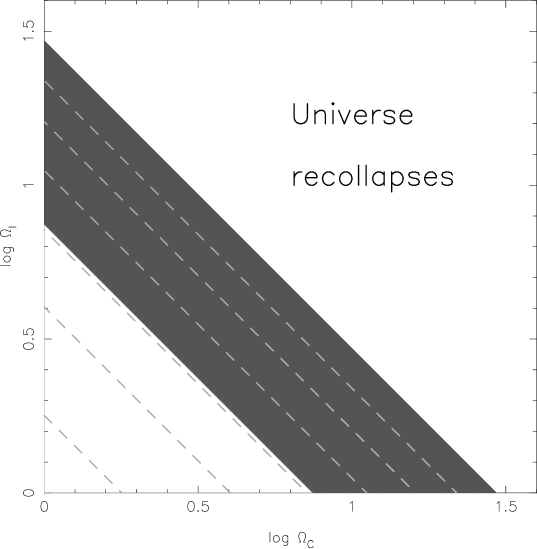
FIG. 4.: The parameter space $\{\Omega_{\ell},\Omega_{C}\}$ is shown for models which exhibit (i) weak loitering: $f(z_{\rm loit})\leq 1/2$ in (50) (lower left corner); (ii) strong loitering: $1/2<f(z_{\rm loit})<1$ in (50) (shaded region). The ‘prohibited’ region corresponding to braneworld models which recollapse before reaching the present epoch is shown on the far right. The dashed lines show contours of $\{\Omega_{\ell}\,,\Omega_{C}\}$ with current values of the effective equation of state: $w_{0}=-1.01,-1.015,-1.02,-1.025,-1.03,-1.035$ (from left to right). All models loiter at $z_{\rm loit}=20$ and have $\Omega_{\rm m}=0.3$.

It is necessary to draw the reader’s attention to the fact that not every set of parameter values gives rise to a ‘realistic’ cosmology. For some of them, the universe recollapses before reaching the present epoch. (The loitering braneworld shares this property with a closed FRW universe, and the reader is referred to [37] for an extensive discussion of this issue.) It is obvious that the model approaches a recollapsing universe as the loitering parameter $f(z_{\rm loit})\to 1$. Thus, setting $f(z_{\rm loit})=1$ in estimate (55), we obtain the approximate boundary of the region of recollapsing universes in the parameter space $\{\Omega_{\ell}\,,\Omega_{C}\}$:

$$\Omega_{C}\Omega_{\ell}\ \lower-1.5pt\vbox{\hbox{\hbox to0.0pt{$>$\hss}\lower 5.3pt\vbox{\hbox{$\sim$}}}}\ \frac{3}{4}\Omega_{\rm m}^{2}(1+z_{\rm loit})^{2}~{},$$ (56)

which corresponds to the ‘prohibited’ region in Fig. 4 for the particular choice of $z_{\rm loit}=20$ and $\Omega_{\rm m}=0.3$.

REFERENCES

- [1] G. T. Richards et al., Astron. J. 127, 1305 (2004), astro-ph/0309274.
- [2] Z. Haiman and E. Quataert, The Formation and Evolution of the First Massive Black Holes, astro-ph/0403225.
- [3] D. N. Spergel, et al., Astrophys. J. Suppl. 148, 175 (2003), astro-ph/0302209; M. Tegmark et al., Phys. Rev. D 69, 103501 (2004).
- [4] R. Barkana and A. Loeb, In the Beginning: The First Sources of Light and the Reionization of the universe, astro-ph/0010468; B. Ciardi and A. Ferrara, The First Cosmic Structures and their Effects, astro-ph/0409018.
- [5] A. Riess et al., Astron. J. 116, 1009 (1998), astro-ph/9805201; S. J. Perlmutter et al., Astrophys. J. 517, 565 (1999), astro-ph/9812133; A. Riess et al., Astrophys. J. 607, 665 (2004), astro-ph/0402512.
- [6] V. Sahni, Dark Matter and Dark Energy, Lectures given at the 2nd Aegean Summer School on the Early universe, Ermoupoli, Island of Syros, Greece, astro-ph/0403324 .
- [7] V. Sahni and Yu. V. Shtanov, JCAP 0311, 014 (2003), astro-ph/0202346; U. Alam and V. Sahni, Supernova Constraints on Braneworld Dark Energy, astro-ph/0209443.
- [8] V. Sahni, H. Feldman, and A. Stebbins, Astrophys. J. 385, 1 (1992).
- [9] V. Sahni and A. A. Starobinsky, Int. J. Mod. Phys. D 9, 373 (2000), astro-ph/9904398.
- [10] S. Alexander, R. Brandenberger, D. Easson, Phys. Rev. D 62, 103509 (2000); R. Brandenberger, D. Easson, D. Kimberley, Nuc. Phys. B623, 421 (2002).
- [11] M. Chevallier and D. Polarski, Int. J. Mod. Phys. D10, 213 (2001) [gr-qc/0009008].
- [12] A. G. Lemaître, MNRAS 91, 483 (1931).
- [13] L. Randall and R. Sundrum, Phys. Rev. Lett. 83, 3370 (1999), hep-ph/9905221; L. Randall and R. Sundrum, Phys. Rev. Lett. 83, 4690 (1999), hep-th/9906064.
- [14] G. Dvali, G. Gabadadze, and M. Porrati, Phys. Lett. B 485, 208 (2000), hep-th/0005016.
- [15] H. Collins and B. Holdom, Phys. Rev. D 62, 105009 (2000), hep-ph/0003173; Yu. V. Shtanov, On Brane-World Cosmology, hep-th/0005193; C. Deffayet, Phys. Lett. B 502, 199 (2001), hep-th/0010186.
- [16] R. M. Wald, General Relativity, University of Chicago Press, Chicago (1984).
- [17] P. Binétruy, C. Deffayet, and D. Langlois, Nucl. Phys. B 565, 269 (2000), hep-th/9905012; C. Csáki, M. Graesser, C. Kolda, and J. Terning, Phys. Lett. B 462, 34 (1999), hep-ph/9906513; J. M. Cline, C. Grojean, and G. Servant, Phys. Rev. Lett. 83, 4245 (1999), hep-ph/9906523; P. Binétruy, C. Deffayet, U. Ellwanger, and D. Langlois, Phys. Lett. B 477, 285 (2000), hep-th/9910219. T. Shiromizu, K. Maeda, and M. Sasaki, Phys. Rev. D 62, 024012 (2001), hep-th/9910076.
- [18] K. Ichiki, M. Yahiro, T. Kajino, M. Orito, and G. J. Mathews, Nucl. Phys. A 718, 386 (2003).
- [19] R. R. Caldwell, M. Kamionkowski, and N. N. Weinberg, Phys. Rev. Lett. 91, 071301 (2003), astro-ph/0302506.
- [20] U. Alam, V. Sahni, and A. A. Starobinsky, JCAP 06, 008 (2004), astro-ph/0403687.
- [21] A. Lue, R. Scoccimarro, and G. D. Starkman, Phys. Rev. D 69, 124015 (2004), astro-ph/0401515.
- [22] U. Seljak et al., Cosmological parameter analysis including SDSS Ly-alpha forest and galaxy bias: constraints on the primordial spectrum of fluctuations, neutrino mass, and dark energy, astro-ph/0407372.
- [23] Yu. Shtanov and V. Sahni, Class. Quantum Grav. 19, L101 (2002), gr-qc/0204040.
- [24] S. Nojiri and S. D. Odintsov, Phys. Lett. B 595, 1 (2004), hep-th/0405078; S. Nojiri and S. D. Odintsov, Phys. Rev. D 70, 103522 (2004), hep-th/0408170; M. C. B. Abdalla, S. Nojiri, and S. D. Odintsov, Consistent modified gravity: dark energy, acceleration and the absence of cosmic doomsday, hep-th/0409177.
- [25] U. Alam, V. Sahni, T. D. Saini and A. A. Starobinsky, MNRAS 344, 1057 (2003), astro-ph/0303009.
- [26] E. V. Linder, Dark Entropy: Holographic Cosmic Acceleration, hep-th/0410017
- [27] A. Kogut, et al., Astrophys. J. Suppl. 148, 161 (2003), astro-ph/0302213.
- [28] D. J. Schwarz, G. D. Starkman, D. Huterer, and C. J. Copi, Phys. Rev. Lett. 93, 221301 (2004), astro-ph/0403353.
- [29] P. J. E. Peebles, Principles of Physical Cosmology, Princeton University Press, Princeton 1993.
- [30] S. Dodelson, Modern Cosmology, Academic Press, 2003.
- [31] A. R. Liddle and D. H. Lyth, Cosmological Inflation and Large-Scale Structure, Cambridge University Press, Cambridge (2000).
- [32] Yun-Song Piao, Bo Feng, and Xinmin Zhang, Phys. Rev. D 69, 103520 (2004), hep-th/0310206.
- [33] C. R. Contaldi, M. Peloso, L. Kofman, and A. Linde, JCAP 0307, 002 (2003), astro-ph/0303636.
- [34] C. L. Bennett et al., Astroph. J. 464, L1 (1996), astro-ph/9601067.
- [35] C. Deffayet, G. Dvali, and G. Gabadadze, Phys. Rev. D 65, 044023 (2002), astro-ph/0105068; C. Deffayet, S. J. Landau, J. Raux, M. Zaldarriaga, and P. Astier, Phys. Rev. D 66, 024019 (2002), astro-ph/0201164.
- [36] A. Padilla, Infra-red modification of gravity from asymmetric branes, hep-th/0410033; A. Padilla, Class. Quantum Grav. 22, 681 (2005), hep-th/0406157.
- [37] J. E. Felten and R. Isaacman, Rev. Mod. Phys. 58, 689 (1986).