A general relativistic approach to the Navarro–Frenk–White galactic halos.

Abstract

Although galactic dark matter halos are basically Newtonian structures, the study of their interplay with large scale cosmic evolution and with relativistic effects, such as gravitational lenses, quintessence sources or gravitational waves, makes it necessary to obtain adequate relativistic descriptions for these self–gravitating systems. With this purpose in mind, we construct a post–Newtonian fluid framework for the “Navarro–Frenk–White” (NFW) models of galactic halos that follow from N–body numerical simulations. Since these simulations are unable to resolve regions very near the halo center, the extrapolation of the fitting formula leads to a spherically averaged “universal” density profile that diverges at the origin. We remove this inconvenient feature by replacing a small central region of the NFW halo with an interior Schwarzschild solution with constant density, continuously matched to the remaining NFW spacetime. A model of a single halo, as an isolated object with finite mass, follows by smoothly matching the NFW spacetime to a Schwarzschild vacuum exterior along the virial radius, the physical “cut–off” customarily imposed, as the mass associated with NFW profiles diverges asymptotically. Numerical simulations assume weakly interacting collisionless particles, hence we suggest that NFW halos approximately satisfy an “ideal gas” type of equation of state, where mass–density is the dominant rest–mass contribution to matter–energy, with the internal energy contribution associated with an anisotropic kinetic pressure. We show that, outside the central core, this pressure and the mass density roughly satisfy a polytropic relation. Since stellar polytropes are the equilibrium configurations in Tsallis’ non–extensive formalism of Statistical Mechanics, we argue that NFW halos might provide a rough empirical estimate of the free parameter $q$ of Tsallis’ formalism.

I Introduction

A large amount of compelling evidence based on direct and indirect observations: rotation velocity profiles, microlensing and tidal effects affecting satellite galaxies and galaxies within galaxy clusters, reveals that most of the matter content of galactic systems is made up of dark matter (DM). Since the physical nature of DM so far remains uncertain, this issue has become one of the most interesting open problems in astrophysics and cosmology KoTu ; Padma1 ; Peac ; Ellis ; Fornengo . Among a wide variety of proposed explanations we have: thermal sources, meaning a colissionless gas of weakly interacting massive particles (WIMP’s), which can be very massive ($m\sim 100-200$ GeV) and supersymmetric Ellis (“cold dark matter” CDM) or self–interacting less massive ($m\sim$ KeV) particles scdm ; wdm (“warm” DM).

The DM contribution dispersed in galactic halos is about 90–95 % of the matter content of galactic systems, while visible baryonic matter (stars and gas) is clustered in galactic disks. It is then a good approximation to consider the gravitational field of a galaxy as that of its DM halo (for whatever assumptions we might make on its physical nature), while visible matter can be thought of as “test particles” in this field HGDM ; Lake .

Assuming the CDM paradigm, we can distinguish two types of halo models: idealized models obtained from a Kinetic Theory approach, whether based on specific theoretical considerations or on convenient ansatzes that fix a distribution function satisfying Vlassov’s equation BT , or models based on “universal” mass density profiles obtained empirically from the outcome of N–body numerical simulations nbody_1 ; nbody_2 ; nbody_3 . In this paper we will study the equilibrium configurations that emerge from the latter approach, based on the well known numerical simulations of Navarro, Frenk and White (NFW) nbody_1 ; LoMa . It is important to mention that these simulations yield virialized equilibrium structures that reasonably fit CDM structures at a cosmological scale ($\gtrsim 100$ Mpc), though some of their predictions in smaller scales (“cuspy” density profiles and excess substructure) seem to be at odds with observations cdm_problems_1 ; cdm_problems_2 , especially those based on galaxies with low surface brightness (LSB), which are supposed to be overwhelmingly dominated by DM and so well suited to examine the predictions of various DM models vera ; LSB .

We consider in this paper that DM halos are spherically symmetric equilibrium configurations, a reasonable approximation since their global rotation is not dynamically significant urc . Galactic halos in virialized equilibrium are also Newtonian systems characterized by typical velocities, ranging from a few km/sec for dwarf galaxies up to about $1000-3000$ km/sec for rich clusters. So, why bother with a general relativistic treatment? First, there is a purely theoretical interest in incorporating these important self–gravitating systems into General Relativity, the best available gravitational theory. In fact, important experimental tests of General Relativity are currently and customarily carried on (within a weak field post–Newtonian approach) in Solar System bound Newtonian systems. Secondly, a post–Newtonian description of galactic halos can be, not only useful and interesting, but essential for studying their interaction with physical effects that lack a Newtonian equivalent, such as gravitational lenses or gravitational waves. In fact, the post–Newtonian halo models that we present in this paper can be readily used in lensing studies, or can provide the unperturbed zero order configuration in the examination of the perturbative effect of gravitational waves on galactic halos. Also, a post–Newtonian description is necessary in the study of the interplay between galactic structures and large scale ($>100\,$ Mpc) cosmological evolution dominated by a repulsive “dark energy”, modeled by sources like quintessence and/or a cosmological constant, whose Newtonian description might be inadequate. Finaly, since galactic halos are customarily examined as Newtonian structures, we feel it is important to show the readership of General Relativity journals how to construct spacetimes, in a post–Newtonian approximation, that are suitable for the description and study of these important self–gravitating systems.

Given the NFW mass density profile, we show in section II how all dynamical variables of the Newtonian NFW halo can be derived. In section III we construct a post–Newtonian fluid relativistic generalization of a NFW halo, under the assumption that the gas of collisionless WIMPs should satisfy an “ideal gas” type of equation of state RKT ; Padma2 ; Padma3 . For isotropic velocity distributions, this assumption allows us to determine the internal energy density by means of the hydrostatic equations themselves. For the case with anisotropic velocities we follow the same procedure with regards to the “radial” component of the stress tensor, determining the “tangential” stress by a suitable empirical ansatz (section VI–B).

The fact that the NFW spherically averaged mass density profile diverges at the halo center follows from interpolating a fitting formula associated with numerical simulations that have a finite resolution limit at the halo center NSres . Although this behavior of the density profile does not imply that simulations predict an infinite central density, it is none–the–less an undesirable feature, which we ammend in section IV by replacing a small region around the center of the NFW halo with a spherical section of a spacetime with constant matter–energy density, i.e. a section of the “interior” Schwarzschild solution, that is continuously matched to the remaining of the NFW post–Newtonian spacetime.

Galactic halos are hierarchical structures: small halos lie within galaxy clusters, which might be part of superclusters, etc, the asymptotic field of a typical NFW halo should somehow merge with a mean field of a larger substructure, or with a mean cosmological field. However, the dynamical input from a suitable cosmological background is well imprinted in the theoretical design of NFW simulations nbody_1 ; nbody_2 ; nbody_3 , while the effect of a cosmological constant on the equilibrium of virialized halo structures is know to be negligible (see SussHdez and references quoted therein). Hence, at galactic scales the empiric NFW profiles are assumed to be valid only up to the “virial radius”, a physical “cut–off” scale associated with a virialization process Padma1 ; Peac ; BT ; Padma2 ; Padma3 , ignoring altogether their transition to background fields associated with larger structures or to a cosmological background. While a post–Newtonian approach also allows one to impose this virial cut–off scale and to ignore its asymptotic behavior, we show in section IV how well behaved asymptotically flat NFW configurations can be constructed. Also, since any localized self–gravitating system (even if belonging to large substructures) can be approximately described as an isolated system, we also examine an alternative cut–off by matching generic NFW halos to a Schwarzschild vacuum exterior at the virial radius.

In section V we provide the equilibrium equations given in terms of suitable dimensionless variables for the post–Newtonian NFW halos, using the matching with the “interior” and “exterior” Schwarzschild solutions defined in section IV. Analytic solutions of these equations are obtained in section VI, for isotropic velocities (subsection A) and for a well defined case with anisotropic velocities (subsection B). We show in both cases that (outside the central region) the radial pressure and mass density satisfy approximately a polytropic relation characteristic of stellar polytropes BT . Even if NFW halos exhibit (in general) deviations from an isotropic velocity distribution, while velocities in polytropes are strictly isotropic, we argue in section VII that the resemblance of outer regions of NFW halos to stellar polytropes might be significant, since virialized self–gravitating systems exhibit non–extensive forms of energy and entropy, and stelar polytropes are the equilibrium states in the application to astrophysical systems of the non–extensive Statistical Mechanics formalism developed by Tsallis Tsallis ; PL ; TS1 ; TS2 (see Chavanis for a critical approach to this formalism).

II The NFW dark matter halos.

The well known N–body numerical simulations by Navarro, Frenk and White (NFW) yield the following “universal” expression for the density profile of virialized galactic halo structures nbody_1 ; nbody_2 ; nbody_3 ; LoMa

$$\rho_{{}_{\mathrm{NFW}}}=\frac{\delta_{0}\,\rho_{0}}{x\,\left(1+x\right)^{2}},$$ (1)

where

$$x = \ \frac{r}{r_{s}},\qquad r_{s}\ =\ \frac{r_{\textrm{\tiny{vir}}}}{c_{0}},$$ (2)

$$\rho_{0} = \ \rho_{\mathrm{crit}}\,\Omega_{0}\,h^{2}\ =\ 253.8\,h^{2}\,\Omega_{0}\,\frac{M_{\odot}}{\text{kpc}^{3}},$$ (3)

$$\delta_{0} = \ \frac{\Delta\,c_{0}^{3}}{3\left[\ln\,(1+c_{0})-c_{0}/(1+c_{0})\right]},$$ (4)

while the concentration parameter $c_{0}$ can be expressed in terms of the virial mass $M_{\textrm{\tiny{vir}}}$ by c0

$$c_{0}=62.1\times\left(\frac{M_{\textrm{\tiny{vir}}}\,h}{M_{\odot}}\right)^{-0.06}\,\left(1+\epsilon\right),$$ (5)

where $-1/3\lesssim\epsilon\lesssim 1/2$. The virial radius $r_{\textrm{\tiny{vir}}}$ is given in terms of $M_{\textrm{\tiny{vir}}}$ by the condition that average halo density equals $\Delta$ times the cosmological density $\rho_{0}$

$$\Delta\,\rho_{0}=\frac{3\,M_{\textrm{\tiny{vir}}}}{4\,\pi\,r_{\textrm{\tiny{vir}}}^{3}},$$ (6)

where $\Delta$ is a model–dependent numerical factor (for a $\Lambda$CDM model with total $\Omega_{0}=1$ we have $\Delta\sim 100$ LoHo ). Hence all quantities depend on a single free parameter $M_{\textrm{\tiny{vir}}}$ with a dispersion range given by $\epsilon$ for different halo concentrations.

Using this profile, the mass function and gravitational potential follow from the Newtonian equations of hydrostatic equilibrium

$$M\,^{\prime}=4\,\pi\,\rho\,r^{2},$$ (7)

$$\Phi\,^{\prime}=\frac{GM}{r^{2}},$$ (8)

where a prime denotes derivative with respect to $r$. Hence, the NFW mass function follows from integrating (7) for $\rho$ given by (1)

$$M_{\textrm{\tiny{NFW}}}=4\,\pi\,r_{s}^{3}\,\delta_{0}\,\rho_{0}\,\left[\ln(1+x)-\frac{x}{1+x}\right],$$ (9)

so that $M_{\textrm{\tiny{NFW}}}(0)=0$, while $M_{\textrm{\tiny{NFW}}}$ evaluated at $r=r_{\textrm{\tiny{vir}}}$    (or $x=c_{0}$) yields $M_{\textrm{\tiny{vir}}}$ as defined in (6) for $\delta_{0}$ given by (4). Circular rotation velocity and the gravitational potential follow from (8)

$$V_{\textrm{\tiny{NFW}}}^{2} =\ V_{0}^{2}\,\,\left[\frac{\ln(1+x)}{x}-\frac{1}{1+x}\right],$$ (10)

$$\Phi_{\textrm{\tiny{NFW}}} =\ -V_{0}^{2}\,\,\frac{\ln\,(1+x)}{x},$$ (11)

where the characteristic velocity $V_{0}$ is

$$V_{0}^{2}\ =\ 4\,\pi\,G\,r_{s}^{2}\delta_{0}\,\rho_{0}\ =\ -\Phi_{\textrm{\tiny{NFW}}}(0)\ =\ \frac{3\delta_{0}}{\Delta c_{0}^{2}}\,\frac{GM_{\textrm{\tiny{vir}}}}{r_{\textrm{\tiny{vir}}}},$$ (12)

and the integration constant was chosen so that $\Phi_{\textrm{\tiny{NFW}}}\to 0$ as $x\to\infty$. Notice that, even if $\rho_{\textrm{\tiny{NFW}}}$ diverges, all other quantities (but not their gradients) are regular as as $x\to 0$.

Since numerical simulations usually yield anisotropic velocity distributions, we have in general an anisotropic stress tensor so that “radial” and “tangential” pressures, $P=P_{r}$ and $P_{\perp}$ are involved in the Navier–Stokes equation

$$P\,^{\prime}=\ -\rho\,\Phi\,^{\prime}-\frac{2\,\Gamma}{r}\,P,$$ (13)

where

$$\Gamma=\frac{P-P_{\perp}}{P},$$ (14)

is the anisotropy factor. Given $\rho_{\textrm{\tiny{NFW}}}$ and $M_{\textrm{\tiny{NFW}}}$, the radial and tangential pressures follow from integrating (13) for a given choice of $\Gamma$. For the NFW forms (1) and (9), there are analytic solutions of (13) for $\Gamma=0$ (isotropic case) and for various empiric forms of $\Gamma$ LoMa .

III Relativistic generalization

Under the assumptions that we outlined in the Introduction, the spacetime metric for an NFW dark matter galactic halo should be a particular case of the spherically symmetric static line element

$$\textrm{d}s^{2}\ =\ -\exp\left(\frac{2\,\Phi}{c^{2}}\right)\,c^{2}\,\textrm{d}t^{2}+\left(1-\frac{2\,G\,M}{c^{2}\,r}\right)^{-1}\,\textrm{d}r^{2}$$

$$+r^{2}(\textrm{d}\theta^{2}+\sin^{2}\theta\,\,\textrm{d}\phi^{2}),$$ (15)

so that $M(r)$ has units of mass. The functions $\Phi(r)$ and $M(r)$ are suitable relativistic generalization of the NFW functions given by (9) and (11). We will assume a fluid energy–momentum tensor of the most general form for the metric (15)

$$T^{ab}=\ \mu\,u^{a}\,u^{b}+p\,h^{ab}+\Pi^{ab},$$ (16)

where $\mu$ and $p$ are the matter–energy density and isotropic pressure along a 4-velocity field $u^{a}=\exp(-\Phi/c^{2})\,\delta^{a}\,_{t}$,  while $h^{ab}=g^{ab}+u^{a}\,u^{b}$ and $\Pi^{ab}$ is the anisotropic and traceless ($\Pi^{a}\,_{a}=0$) stress tensor, which for the metric (15) takes the form

$$\Pi^{a}\,_{b}\ =\ \textbf{diag}\,[0,\,-2\Pi,\,\Pi,\,\Pi]$$ (17)

so that $p$ and $\Pi=\Pi(r)$ relate to the radial and tangential pressures, $P$ and $P_{\perp}$, by

$$P_{\perp}-P\ =\ 3\,\Pi,\qquad 2\,P_{\perp}+P\ =\ 3\,p.$$ (18)

The field equations and momentum balance ($T^{ab}\,_{;b}=0$) associated with (15)-(18) are

$$M\,^{\prime} =\ 4\,\pi\,\mu\,r^{2}/c^{2},$$ (19)

$$\Phi\,^{\prime} =\ \frac{G\,[M+4\,\pi\,P\,r^{3}/c^{2}]}{r\,\left[r-2\,G\,M/c^{2}\right]},$$ (20)

$$P\,^{\prime} =\ -(\mu+P)\,\frac{\Phi\,^{\prime}}{c^{2}}-\frac{2\,\Gamma}{r}\,P,$$ (21)

where $\Gamma$ is given by (14). These equations are the relativistic generalization of the Newtonian equilibrium equations (7), (8) and (13). In the Newtonian case all these equations are decoupled, so that once $\rho$ is known and $\Gamma$ is prescribed, all other quantities follow by simple integration of quadratures. In the relativistic case we have, in general, three equations for five unknowns ($\mu,\,P,\,\Gamma,\,M,\,\Phi$). Thus, we must provide a relation between $\mu$ and $P$, together with a suitable assumption that determines or prescribes the form of $\Gamma$.

Since the WIMPs in the collisionless gas making up galactic halos are interacting very weakly, it is reasonable to consider such a gas as approximately an “ideal gas” whose total matter–energy density, $\mu$, is the sum of a dominant contribution from rest–mass density, $\rho\,c^{2}$, and an internal energy term that is proportional to the pressure $P$ and to the velocity dispersion $\sigma^{2}=\langle v^{2}\rangle\simeq\langle v_{\perp}^{2}\rangle$. Hence, we shall assume that the matter source of NFW halos complies with the equation of state of a non–relativistic (but non–Newtonian) ideal gas Peac ; RKT ; Padma2 ; Padma3

$$\mu\ =\ \rho\,c^{2}\,\left[1+\frac{3}{2}\,\frac{\sigma^{2}}{c^{2}}\right],\qquad P\ =\ \rho\,\sigma^{2},$$ (22)

where we can identify $\rho=\rho_{\textrm{\tiny{NFW}}}$ (or with any mass density formula used in halo models) and the velocity dispersion is related to a kinetic temperature $T$ by BT

$$\sigma^{2}\ =\ \frac{P}{\rho}\ =\ \frac{k_{{}_{B}}\,T}{m},$$ (23)

where $k_{{}_{B}}$ is Boltzmann’s constant. At this point, we believe it is convenient to mention the following two idealized models of self–gravitating systems as useful theoretical references BT :

Isothermal Sphere:

$$\sigma^{2}=\frac{k_{{}_{B}}\,T_{0}}{m}=\textrm{const.}\quad\Rightarrow\quad P=K\,\rho,\qquad$$

Stellar Polytropes:

$$\sigma^{2}=K\,\rho^{1/n}\quad\quad\,\Rightarrow\quad P=K\,\rho^{1+1/n},\qquad$$ (24)

where $T_{0}$, $K$ and $n$ (polytropic index) are constants. The isothermal sphere corresponds to a Maxwell–Boltzmann velocity distribution, the equilibrium state associated with the extensive Boltzmann–Gibbs entropy BT ; Padma2 ; Padma3 . The stellar polytropes are also solutions of the Vlassov equation, but are associated with the equilibrium state in the non–extensive entropy functional proposed by Tsallis Tsallis ; PL ; TS1 ; TS2 . Notice that the isothermal sphere follows from the stellar polytropes in the limit $n\to\infty$ (the extensivity limit in Tsallis’ formalism).

For Newtonian characteristic velocities in galactic halos, we have $\sigma^{2}/c^{2}\ll 1$ and $\mu\approx\rho\,c^{2}$ and so $P\simeq P_{\perp}\ll\rho\,c^{2}$, so that (22) provides a plausible equation of state for a relativistic generalization of galactic halos. It is evident that in the Newtonian limit $\sigma^{2}/c^{2}\to 0$ we recover the Newtonian equilibrium equations (7), (8) and (13). What needs to be done now is to insert the equation of state (22) into the field equations (19)–(21). It turns out to be easier to work with $P$ instead of $\sigma$ or $T$, using (22) as

$$\mu\ =\ \rho\,c^{2}+\frac{3}{2}\,P,$$ (25)

so that $\sigma$ and/or $T$ can be obtained afterwards from $P$ through (22) and (23). Combining (20) and (21) into a single equation and using (25) we obtain the set

$$M^{\prime} = \ 4\,\pi\,\left[\rho+\frac{3}{2}\,\frac{P}{c^{2}}\right]\,r^{2},$$ (26)

$$P^{\prime} = \ -\frac{G[\rho+\frac{5}{2}P/c^{2}]\,[M+4\pi\,(P/c^{2})\,r^{3}]}{r[r-(2G/c^{2})\,M]}-\frac{2\,\Gamma}{r}\,P,$$

which becomes determined once we identify $\rho=\rho_{\textrm{\tiny{NFW}}}$ and specify $\Gamma=\Gamma(r)$. We can solve these equations in a post–Newtonian approximation by keeping only terms up to order $\sigma^{2}/c^{2}$.

IV Providing a regular center and matching with a Schwarzschild exterior

By looking at (1), it is evident that $\rho=\rho_{\textrm{\tiny{NFW}}}$ diverges as $r\to 0$. A careless examination, from a full general relativistic point of view, of the spherical spacetime given by (15)–(22) with $\rho=\rho_{\textrm{\tiny{NFW}}}$, would yield a curvature singularity marked by $r=0$, associated with the blowing up of the Ricci scalar

$$R\ =\ \frac{8\pi G}{c^{4}}\,\left[\rho_{\textrm{\tiny{NFW}}}\,c^{2}+\left(2\,\Gamma-\frac{3}{2}\right)\,P\right].$$ (28)

However, this situation does not apply to NFW halos, not only because they are Newtonian systems that must be examined within the framework of a Newtonian limit of a weak field approach, but because the NFW mass density profile (1) is an empirical fitting formula that emerges from spherically averaging numerical simulations that cannot resolve distances smaller than about 1 % of the actual physical radius of the halo NSres . Hence, astrophysicists using this density profile do not actually assume infinite central densities, but regard this blowing up of $\rho_{\textrm{\tiny{NFW}}}$ as an undesired effect due to the extrapolation of a fitting formula which (within the resolution limits of numerical simulations) provides a rough illustration of the fact that density becomes “cuspy” along the central halo region, i.e. $\rho_{\textrm{\tiny{NFW}}}\sim 1/x$ for $x\ll 1$.

A practical way to get rid of this inconvenient feature is to “replace” a small spherical region $0<x<x_{0}$ of the NFW spacetime with an “inner” fluid region containing the world–line of a regular center. Using the definitions (2)–(6), the radius $r_{0}$ of this inner region in terms of $M_{\textrm{\tiny{vir}}}$ is given by

$$\frac{r_{0}}{\textrm{kpc}}\ =\ 0.272\,\times\,\left(\frac{M_{\textrm{\tiny{vir}}}}{M_{\odot}}\right)^{0.273}\,x_{0}.$$ (29)

Hence, for halos in the observed range $10^{8}\,M_{\odot}<M_{\textrm{\tiny{vir}}}<10^{15}\,M_{\odot}$, the choice $x_{0}=0.0001$ yields $4\,\textrm{pc}\lesssim r_{0}\lesssim 340\,\textrm{pc}$, a very small radius in relation to the virial radii of these halos. Thus, since this length scale is much smaller than the maximal resolution of numerical simulations NSres , we are able to provide a regular center for the NFW spacetime but this does not prevent us from studying the effects of its steep density profile in the central region.

The simplest choice of a spacetime geometry for the inner region is a section of a Schwarzschild interior solution Steph characterized by the metric (15) with

$$\exp\,\left(\frac{\Phi}{c^{2}}\right) = a_{0}-b_{0}\,\sqrt{1-\kappa_{0}\,r^{2}}$$

$$M = \frac{4\,\pi\,\mu_{c}}{3\,c^{2}}\,r^{3},$$ (30)

with $\kappa_{0}=8\,\pi\,G\,\mu_{c}/c^{4}$ and

$$\mu = \mu_{c}\ =\ \textrm{const.},$$ (31)

$$P = \frac{\mu_{c}}{3}\,\frac{3\,b_{0}\,\sqrt{1-\kappa_{0}\,r^{2}}-a_{0}}{a_{0}-b_{0}\,\sqrt{1-\kappa_{0}\,r^{2}}},$$ (32)

where the constants $a_{0},\,b_{0}$ and $\mu_{c}$ must be selected so that this region can be suitably “glued” to the NFW spacetime occupying $x>x_{0}$.

As we mentioned before, it is customary to disregard the asymptotic behavior of NFW profiles, since the virial radius is considered to be the physical cut–off radius of NFW halos. However, we can construct asymptotically well behaved NFW configurations for which $\mu,\,P,\,M/r$ and $\Phi$ tend to zero as $x\to\infty$ (though $M$ most certainly will diverge in this limit, since the Newtonian $M_{\textrm{\tiny{NFW}}}$ in (9) already does). A finite $M$ as $r\to\infty$ can be achieved if we match the NFW spacetime at a convenient cut–off scale to a Schwarzschild vacuum exterior characterized by $\mu=P=0$ and by (15) with

$$\exp\,\left(\frac{2\,\Phi}{c^{2}}\right)\ =\ 1-\frac{2\,G\,M_{0}}{c^{2}\,r},\qquad M\ =\ M_{0},$$ (33)

where $M_{0}$ is the constant “Schwarzschild mass”.

Necessary conditions for a smooth matching between spacetime regions are given by Darmois matching conditions seno , requiring continuity of the induced metric and extrinsic curvature of the matching hypersurface

$$h_{ab}=n_{a}\,n_{b}-g_{ab},\qquad K_{ab}=-h_{a}^{c}\,h_{b}^{d}\,n_{c;d},$$ (34)

where $n^{a}$ is a unit vector normal to this hypersurface. Since the NFW spacetime must be matched, either to (30) or to (33), at hypersurfaces marked by constant $r$, we have $n_{a}=\sqrt{g_{rr}}\,\delta_{a}^{r}$, hence (34) imply that $g_{tt},\,g_{tt}^{\prime}$ and $g_{rr}$ (but not necessarily $g_{rr}^{\prime}$) must be continuous at the matching hypersurface. Considering (19)–(21), this implies continuity at the matching hypersurface of $M,\,\Phi$ and $P$, but not of $\mu$ or the anisotropic pressure defined in terms of $\Gamma$ by (14).

IV.1 Matching with the inner region.

It is convenient to assume (25) to be valid at $r=0$, so that we can characterize the Schwarzschild interior solution by

$$\mu_{c}\ =\ \rho_{c}\,c^{2}+(3/2)\,P_{c},$$ (35)

Following (12), we can define a characteristic velocity

$$V_{c}^{2}\ =\ 4\,\pi\,G\,\rho_{c}\,r_{s}^{2},$$ (36)

so that

$$P_{c}\ =\ \delta_{c}\,\rho_{c}\,V_{c}^{2},\qquad\xi\ =\ \frac{P_{c}}{\rho_{c}\,c^{2}}\ =\ \delta_{c}\,\frac{V_{c}^{2}}{c^{2}},$$ (37)

where $\delta_{c}$ is an arbitrary constant, so that central velocity dispersion is $\sigma_{c}^{2}=\delta_{c}\,V_{c}^{2}$. Hence, for $0\leq x\leq x_{0}$ we have

$$M\ =\ \frac{4\,\pi}{3}\,\rho_{c}\,\left(1+\frac{3}{2}\,\xi\right)\,r_{s}^{3}\,x^{3},$$ (38)

while, for the time being, we assume also $\Gamma=0$, though a nonzero $\Gamma$ can be considered for the inner region in the case of anisotropic pressure (see section VI–B). Since we are considering $x<x_{0}\sim 0.0001\ll 1$, suitable expressions for the remaining variables in this region are found by expressing $a_{0},\,b_{0}$ in terms of the parameters in (35)–(36) and expanding (30) and (32) up to first order in $x^{2}$, leading to

$$\Phi\ \approx \ \Phi_{c}+\frac{1}{6}\,V_{c}^{2}\,\left(1+\frac{9}{2}\,\xi\right)\,x^{2},$$ (39)

$$P\ \approx \ \rho_{c}\,V_{c}^{2}\left[\delta_{c}-\frac{1}{6}\,\left(1+\frac{5}{2}\,\xi\right)\,\left(1+\frac{9}{2}\,\xi\right)\,x^{2}\right],$$

$$V_{\textrm{\tiny{rot}}}^{2} = r\,\Phi^{\prime}\ \approx\ \frac{1}{3}\,V_{c}^{2}\,\left(1+\frac{3}{2}\,\xi\right)\,x^{2},$$ (41)

Following the matching conditions (34), the constants $\rho_{c},\,V_{c},\Phi_{c}$ and $\delta_{c}$ must be selected so that $M(x_{0}),\,\Phi(x_{0})$ and $P(x_{0})$ continuously match the NFW functions $M,\,\Phi$ and $P$ at $x_{0}$. Although, (34) do not require this continuity for $\mu$ and $\Gamma$, we will still assume it in order to avoid an unphysical jump discontinuity of these variables at $x=x_{0}$, as well as all state variables.

IV.2 Matching with a vacuum exterior.

A smooth matching with a Schwarzschild exterior at a cut–off radius $r=r_{b}$ based on (34) requires

$$M(r_{b}) = M_{0},\quad\textrm{e}^{2\Phi(r_{b})/c^{2}}=1-\frac{2\,G\,M_{0}}{r_{b}},$$ (42)

$$P(r_{b}) = 0,$$ (43)

but do not require $\mu$ or $\Gamma$ to vanish at $r_{b}$. However, a jump discontinuity of these variables at an interface with a vacuum exterior is much more acceptable than in the interface between two non–vacuum regions. As we discuss in section VI, a convenient cut–off scale for a NFW spacetime is the virial radius $r_{b}=r_{\textrm{\tiny{vir}}}$, so that we can identify $M_{0}$ with $M_{\textrm{\tiny{vir}}}$. Though, because of the matching with the inner region, an $r_{\textrm{\tiny{vir}}}$ selected by means of condition (43) will not yield (even in the Newtonian limit) $M_{0}=M_{\textrm{\tiny{vir}}}$ with $M_{\textrm{\tiny{vir}}}$ given by (6). However, for sufficiently small $x_{0}\ll 1$ the resulting $M_{0}$ will be approximately equal to $M_{\textrm{\tiny{vir}}}$.

V Post–Newtonian NFW halos

In order to explore the post–Newtonian limit for the system (26)–(LABEL:P3r), it is useful to work with dimensionless variables by rescaling all variables in terms of quantities defined at the scale radius $r_{s}$.

V.1 The region $x>x_{0}$

Convenient rescalings follow as

$$Y\ = \ \frac{\rho_{\textrm{\tiny{NFW}}}}{\delta_{0}\,\rho_{0}}\ =\ \frac{1}{x\,[1+x]^{2}},$$ (44)

$${\cal{M}}\ = \ \frac{M}{4\,\pi\,\delta_{0}\,\rho_{0}\,r_{s}^{3}}\ =\ \frac{c_{0}^{3}\,\Delta\,M}{3\,\delta_{0}\,M_{\textrm{\tiny{vir}}}},$$ (45)

$${\cal{P}}\ = \ \frac{P}{\delta_{0}\,\rho_{0}\,V_{0}^{2}},$$ (46)

$$\Psi\ = \ \frac{\Phi-\Phi_{c}}{V_{0}^{2}},$$ (47)

with $V_{0}$ defined in (12), transforming (26) and (LABEL:P3r) into

$$\frac{\textrm{d}{\cal{M}}}{\textrm{d}x} =\ \left[Y+\frac{3}{2}\,\varepsilon\,{\cal{P}}\right]\,x^{2},$$ (48)

$$\frac{\textrm{d}{\cal{P}}}{\textrm{d}x} =\ -\frac{\left[Y+\frac{5}{2}\,\varepsilon\,{\cal{P}}\right]\,\left[{\cal{M}}+\varepsilon\,{\cal{P}}\,x^{3}\right]}{x\,\left[x-2\,\varepsilon\,{\cal{M}}\right]}-\frac{2\Gamma}{x}\,{\cal{P}},$$

where

$$\varepsilon\ =\ \frac{V_{0}^{2}}{c^{2}},$$ (50)

so that in the limit $\varepsilon\to 0$ we recover the Newtonian equations (7), (8) and (13). The system (48)–(LABEL:Px) can be integrated by demanding that ${\cal{M}}$ and ${\cal{P}}$ comply with appropriate boundary and initial conditions, so that the NFW halo can be smoothly matched with the Schwarzschild interior at $x=x_{0}$ and the Schwarzschild exterior at $r=r_{\textrm{\tiny{vir}}}$. Since we have to use the explicit form of $Y$ in (44), then the analytic or numerical solutions of (48)–(LABEL:Px) for specific choices of $\Gamma$, boundary conditions depend on $M_{\textrm{\tiny{vir}}}$ through the definitions (4) and (5).

The metric function $M=V_{0}^{2}\,r_{s}\,{\cal{M}}$ follows from (48), while $\Phi=\Phi_{c}+V_{0}^{2}\,\Psi$ can be obtained by integrating

$$\frac{\textrm{d}\,\Psi}{\textrm{d}x}\ =\ \frac{{\cal{M}}+\varepsilon\,{\cal{P}}\,x^{3}}{x\,[x-2\,\varepsilon\,{\cal{M}}]}.$$ (51)

The relativistic generalization of the Newtonian rotation velocity profile are the velocities of test observers along circular geodesics. These velocities are HGDM ; Lake $V_{\textrm{\tiny{rot}}}^{2}=r\,\Phi^{\prime}$, which in terms of the dimensionless variables becomes

$${\cal{V}}^{2}\ =\ \frac{V_{\textrm{\tiny{rot}}}^{2}}{V_{0}^{2}}\ =\ \frac{{\cal{M}}+\varepsilon\,{\cal{P}}\,x^{3}}{x-2\,\varepsilon\,{\cal{M}}}$$ (52)

Since $V_{0}$ for typical galactic halos ranges from a few km/sec to $\sim 1500$ km/sec, the post–Newtonian corrections of order $V_{0}^{2}/c^{2}$ will be very small: between $O(\varepsilon)\sim 10^{-9}$ and $O(\varepsilon)\sim 10^{-6}$. The post–Newtonian system associated with (48)–(LABEL:Px) can be given as

$$\frac{\textrm{d}{\cal{M}}}{\textrm{d}x} = \ Y\,x^{2}+O(\varepsilon),$$ (53)

$$\frac{\textrm{d}{\cal{P}}}{\textrm{d}x} = \ -\frac{Y\,{\cal{M}}}{x^{2}}-\frac{2\Gamma}{x}\,{\cal{P}}+O(\varepsilon),$$ (54)

with

$$\frac{\textrm{d}\,\Psi}{\textrm{d}x}\ =\ \frac{{\cal{M}}}{x^{2}}+O(\varepsilon),$$ (55)

$${\cal{V}}\,^{2}\ =\ \frac{{\cal{M}}}{x}+O(\varepsilon)$$ (56)

V.2 The region $0\leq x\leq x_{0}$

The variables defined in the previous subsection must glue continuously at $x_{0}$ with the interior Schwarzschild variables (35)–(LABEL:P_intS). Normalizing these variables with the same factors as in (44)–(46), we have in the region $x\leq x\leq x_{0}$

$$Y = Y_{0}\ =\ \frac{\rho_{c}}{\delta_{0}\,\rho_{0}}\ =\ \frac{\xi}{\delta_{c}\,\varepsilon}\ =\ \frac{1}{x_{0}\,(1+x_{0})^{2}},$$ (57)

$${\cal{M}} = \frac{1}{3}\,Y_{0}\,\left[1+\frac{3}{2}\,\xi\right]\,x^{3},$$ (58)

$${\cal{P}} \approx Y_{0}^{2}\,\left[\delta_{c}-\frac{1}{6}\,\left(1+\frac{5}{2}\,\xi\right)\,\left(1+\frac{9}{2}\,\xi\right)\,x^{2}\right],$$

$$\Psi \approx \frac{1}{6}\,Y_{0}\,\left(1+\frac{9}{2}\,\xi\right)\,x^{2},$$ (60)

$${\cal{V}}\,^{2} \approx \frac{1}{3}\,Y_{0}^{2}\,\left(1+\frac{3}{2}\,\xi\right)\,x^{2}.$$ (61)

From (57) and bearing in mind that $x_{0}\ll 1$, we have

$$\xi\ \approx\ \frac{\varepsilon\,\delta_{c}}{x_{0}},$$ (62)

implying that $\xi\sim\varepsilon$ if $\delta_{c}\sim x_{0}$. Since $\varepsilon$ is very small we can also assume that $\xi\ll 1$, so that post–Newtonian expressions follow by taking only terms up to $O(\xi)$:

$${\cal{M}} = \frac{1}{3}\,Y_{0}\,x^{3}+O(\xi),$$ (63)

$${\cal{P}} = Y_{0}^{2}\,\left[\delta_{c}-\frac{1}{6}\,x^{2}\right]+O(\xi),$$ (64)

$$\Psi = \frac{1}{6}\,Y_{0}\,x^{2}+O(\xi),$$ (65)

$${\cal{V}}\,^{2} = \frac{1}{3}\,Y_{0}^{2}\,x^{2}+O(\xi).$$ (66)

We examine analytic solutions of the post–Newtonian system (53)–(54) that match continuously with (63)–(65).

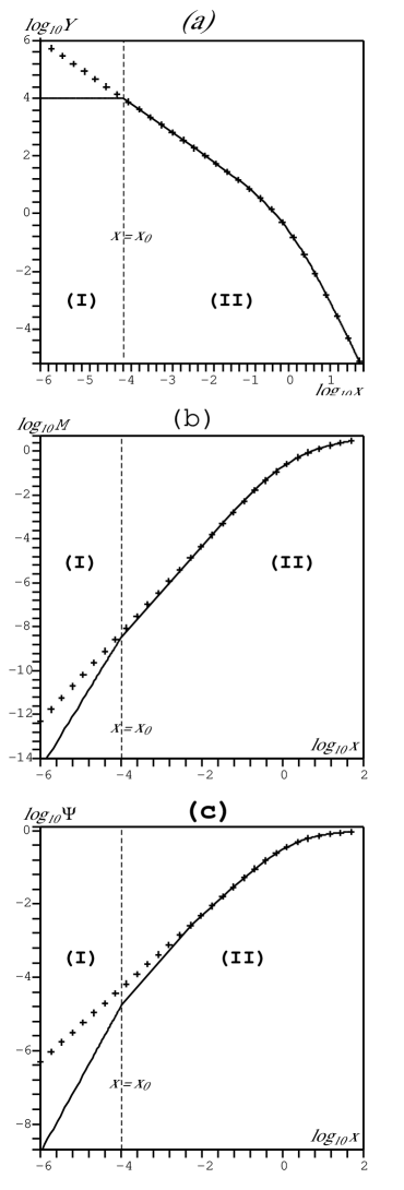
Figure 1: Solid curves in panels (a), (b) and (b) respectively depict the logarithmic plots of $Y,\,{\cal{M}}$ and $\Psi$ given by (44), (57), (LABEL:eq_M) and (69), in the inner (I) and outer (II) regions separated by $x_{0}=0.0001$. In each panel the “pure” NFW case without inner region is shown by the curves with crosses. Notice how this latter case is practically identical to $Y,\,{\cal{M}}$ and $\Psi$ in the outer region.

VI Analytic solutions.

For whatever choice of $\Gamma$ and restrictions on $P$, equations (53) and (55) can be integrated, yielding ${\cal{M}}$ and $\Phi$ so that ${\cal{M}}(x_{0})$ and $\Phi(x_{0})$ match (63) and (65) at $x=x_{0}$. Denoting the inner and NFW regions as

$$0\ \leq\ x\ \leq\ x_{0},\qquad\textrm{(I)},$$

$$x\ >\ x_{0},\qquad\textrm{(II)}.$$ (67)

We have then the following solutions up to orders $O(\varepsilon)\sim O(\xi)$:

$${\cal{M}}_{\textrm{(I)}} = \frac{x^{3}}{3\,x_{0}\,(1+x_{0})^{2}}+O(\xi),$$

$${\cal{M}}_{\textrm{(II)}} = \frac{(3+4x_{0})\,x_{0}}{3\,(1+x_{0})^{2}}+\ln\,\frac{1+x}{1+x_{0}}-\frac{x}{1+x}+O(\varepsilon),$$

$$\Psi_{\textrm{(I)}} = \frac{x^{2}}{6\,x_{0}(1+x_{0})^{2}}+O(\xi),$$

$$\Psi_{\textrm{(II)}} = \frac{2+3\,x_{0}}{2\,(1+x_{0})^{2}}+\frac{1}{x}\,\left[\ln\,\frac{1+x}{1+x_{0}}-\frac{(3+4\,x_{0})\,x_{0}}{3\,(1+x_{0})^{2}}\right]$$ (69)

$$+O(\varepsilon),$$

Therefore, irrespective of the choice of $\Gamma$ and/or assumptions on $P$, the metric elements for all NFW halo spacetimes are up to order $\varepsilon^{2}$

$$-g_{tt} = \textrm{e}^{2\Phi_{c}/c^{2}}\textrm{e}^{2\varepsilon\,\Psi}=1+\frac{2\Phi_{c}}{c^{2}}+2\,\varepsilon\Psi+O(\varepsilon^{2}),$$

$$g_{rr} = \left[1-\frac{2\,\varepsilon\,{\cal{M}}}{x}\right]^{-1}=1+\frac{2\,\varepsilon\,{\cal{M}}}{x}+O(\varepsilon^{2}),$$ (71)

where the metric functions ${\cal{M}}$ and $\Psi$ are given by (LABEL:eq_M) and (69) in the regions (I) and (II), and we have obtained $M$ and $\Phi$ from ${\cal{M}}$ and $\Psi$ by means of (45) and (60). Figures 1a, 1b and 1c display the normalized density $Y$ and the metric functions ${\cal{M}}$ and $\Psi$ in regions (I) and (II).

Notice that all functions defined so far reduce to their Newtonian NFW forms, as given in section II, in the limits $x_{0}\to 0$ and $\varepsilon\to 0$. Also, while all NFW halos have the same rest–mass density $Y$, the form for the pressure depends on the assumptions one might make about $\Gamma$ and suitable boundary conditions.

VI.1 Isotropic case

For $\Gamma=0$ we have $P=P_{r}=P_{\perp}$ and so pressure is isotropic. In collisionless systems this implies an isotropic distribution of velocity dispersion. In this case, (54) yields the following analytic solution

$${\cal{P}}_{\textrm{(I)}} = \frac{\delta_{c}-x^{2}/6}{x_{0}^{2}\,(1+x_{0})^{4}}+O(\xi)$$

$${\cal{P}}_{\textrm{(II)}} = \frac{\delta_{c}-x_{0}^{2}/6}{x_{0}^{2}\,(1+x_{0})^{4}}+{\cal{F}}-{\cal{F}}_{0}+O(\varepsilon),$$ (72)

where ${\cal{F}}_{0}$ is the evaluation at $x=x_{0}$ of the function

$${\cal{F}} = {\cal{F}}(x_{0},x)\ =\ \frac{3}{2}\,\left[\ln\,(1+x)\right]^{2}+\left[\,A_{1}-\alpha_{0}\,\right]\,\ln\,(1+x)+\left[\alpha_{0}-7/2\right]\,\ln x+3\,\textrm{Li}_{2}\,(1+x)+\alpha_{0}\,B_{1}+C_{1},$$ (73)

$$\alpha_{0} = 3\ln(1+x_{0})+\frac{3(1+x_{0})-x_{0}^{2}}{(1+x_{0})^{2}},\quad A_{1}=\frac{1-3x+x^{2}+7x^{3}}{2x^{2}(1+x)}\quad B_{1}=\frac{1-3x-6x^{2}}{2x^{2}(1+x)},\quad C_{1}=\frac{1-3x-18x^{2}-13x^{3}}{2x^{2}(1+x)^{2}}$$

and the dilogarithmic function is defined as

$$\textrm{Li}_{2}(y)\ =\ \int_{1}^{y}{\frac{\ln t\,\textrm{d}t}{1-t}}.$$

This form of ${\cal{P}}$ matches continuously the regions (I) and (II). Since the limit of ${\cal{F}}(x,x_{0})$ as $x\to\infty$ depends explicitly on $x_{0}$ and $\delta_{c}$, we need to find appropriate relations $\delta_{c}=\delta_{c}(x_{0})$ in order to determine (together with (LABEL:eq_M)–(71)) the asymptotic behavior of the NFW spacetime.

Figure 2: Logarithmic plot of normalized pressure ${\cal{P}}$ in regions (I) and (II) with $x_{0}=0.0001$. Panels (a) and (b) respectively denote the isotropic (eqs (72)–(73)) and anisotropic (eqs (82)–(LABEL:Qdef)) cases. The letters A and S depict the asymptotically flat case that scales as  $\ln\,x/x^{4}$  and the case with a matching with a Schwarzschild exterior at the virial radius ($x=c_{0}=15$) so that ${\cal{P}}(c_{0})=0$. The dotted curves in the inner regions are the NFW cases without an inner region. In the anisotropic case we have chosen $\beta=20$. The curves deviating from A correspond to cases that scale asymptotically as $x^{-2}$

VI.1.1 Asymptotically flat configuration

The asymptotic behavior ($x\gg 1$) of (72)–(73) is given by

$${\cal{P}}_{\textrm{(II)}} = \frac{\delta_{c}-x_{0}^{2}/6}{x_{0}^{2}\,(1+x_{0})^{4}}-{\cal{F}}_{0}-\frac{\pi^{2}}{2}$$ (74)

$$+ \frac{1-(3/4)\,\alpha_{0}+4\,\ln\,x}{16\,x^{4}}+O\left(\frac{\ln x}{x^{5}}\right),$$

Since in region (II) we have:  $\rho\to 0$ as $x\to\infty$, an asymptotically flat NFW configuration without cut–off scales requires that ${\cal{P}}_{\textrm{(II)}}\to 0$ as $x\to\infty$, thus the zero order term in (74) must vanish, leading to

$$\delta_{c} = \frac{x_{0}^{2}}{6}\left[1+6\,(1+x_{0})^{4}\left({\cal{F}}_{0}+\frac{\pi^{2}}{2}\right)\right],$$ (75)

$$\approx \left[\ln\,\frac{1}{\sqrt{x_{0}}}+\frac{\pi^{2}}{2}-\frac{17}{3}\right]\,x_{0}^{2}\ \approx\ x_{0}^{2}\,\ln\,\frac{1}{\sqrt{x_{0}}},$$

where we have used (73) and the fact that $x_{0}\ll 1$ in order to get this leading term expansion on $x_{0}$. Hence, (62) implies that $\xi$ is smaller than $\varepsilon$ but of the same order of magnitude, so that $O(\xi)\sim O(\varepsilon)$. The asymptotic limit given by (74)–(75) also implies $\Psi_{\textrm{(II)}}\to 0$ and, even if ${\cal{M}}_{\textrm{(II)}}$ diverges, we have ${\cal{M}}/x\to\ln(x)/x\to 0$ so that asymptotically we have also $g_{rr}\to 1$.

VI.1.2 Matching with a vacuum exterior.

For a galactic halo structure the cut–off scale for a matching with a Schwarzschild exterior should be the virial radius $r=r_{\textrm{\tiny{vir}}}$ (equivalently, $x=c_{0}$), hence condition (43) implies

$${\cal{P}}_{\textrm{(II)}}(c_{0})\ = \ 0,$$

$$\quad\Rightarrow\quad\delta_{c}\ = \ \frac{x_{0}^{2}}{6}\left[1+6\,(1+x_{0})^{4}\,({\cal{F}}(c_{0})-{\cal{F}}_{0})\right],$$

$${\cal{P}}_{\textrm{(II)}}\ = \ {\cal{F}}-{\cal{F}}(c_{0})$$ (76)

where ${\cal{F}}(c_{0})$ is $F(x_{0},x)$ evaluated at $x=c_{0}$. For $h=0.7$ and bearing in mind that for all virialized galactic halo structures we have  $10\,^{8}\lesssim M_{\textrm{\tiny{vir}}}/M_{\odot}\lesssim 10^{15}$,  numerical values of $c_{0}$ given by (5) fall in the range $6\lesssim c_{0}\lesssim 30$. Thus, considering the function ${\cal{F}}$ in (73) we can expand $\delta_{c}$ as in (75), leading to

$$\delta_{c}\ \approx\ \left[\ln\,\frac{1}{\sqrt{x_{0}}}-0.73\right]\,x_{0}^{2}\ \approx\ x_{0}^{2}\,\ln\,\frac{1}{\sqrt{x_{0}}},$$ (77)

so that $\delta_{c}$ is of the same order of magnitude as in (77). Conditions (42) for the post–Newtonian metric functions (LABEL:eq_M)–(71) are given by

$$\frac{\Phi_{c}}{c^{2}}+\varepsilon\,\Psi(c_{0})=\varepsilon\,\frac{{\cal{M}}(c_{0})}{c_{0}},\qquad{\cal{M}}(c_{0})=\frac{M(r_{\textrm{\tiny{vir}}})}{4\pi\delta_{0}\rho_{0}r_{s}^{3}},$$

which imply

$$\frac{\Phi_{c}}{c^{2}} = -\varepsilon\left[\frac{2+3x_{0}}{2(1+x_{0})^{2}}+\frac{2}{c_{0}}\ln\,\frac{1+c_{0}}{1+x_{0}}-\frac{1}{1+c_{0}}\right]+O(\varepsilon^{2})\ \approx\ -\varepsilon\left[1+\frac{2\,\ln(1+c_{0})}{c_{0}}-\frac{1}{1+c_{0}}\right],$$ (79)

$$M(r_{\textrm{\tiny{vir}}}) = M_{\textrm{\tiny{vir}}}\left[1+\frac{3\delta_{0}}{\Delta c_{0}^{3}}\left(\ln(1+x_{0})-\frac{(3+4x_{0}^{2})x_{0}}{3(1+x_{0})^{2}}\right)+O(\varepsilon)\right]\ \approx\ M_{\textrm{\tiny{vir}}},$$ (80)

where we have used the definitions of $\delta_{0},\,M_{\textrm{\tiny{vir}}}$ in (4) and (6). Notice that, because of the matching with an inner region, $M(r_{\textrm{\tiny{vir}}})=M_{\textrm{\tiny{vir}}}$ does not hold exactly in the Newtonian limit, though it holds for a very good approximation if $x_{0}$ is sufficiently small. We show in figure 2a the logarithmic plot of ${\cal{P}}(x)$ for the two cases considered above (asymptotically flat and matched to a Schwarzschild exterior).

VI.1.3 Polytropic equation of state.

The complexity of the expressions in (72) and (73) do not allow us to find out, at first glance, the type of relation between $P$ and $\rho$. Though, by looking at (44) and (74), the asymptotic behavior ${\cal{P}}\sim\ln(x)/x^{4}\sim 1/x^{4}$ and $Y\sim 1/x^{3}$ indicates a sort of power law relation between ${\cal{P}}$ and $Y$ that (at least asymptotically) might be similar to the polytropic relation (24). In order to examine the functional relation between $Y$ and ${\cal{P}}$, we provide in figure 3a the logarithmic plot of ${\cal{P}}$ vs $Y$ (or equivalently $\ln P$ vs $\rho\,V_{0}^{2}$), for the asymptotically flat case and the case matched with a Schwarzschild exterior, using the numerical values $x_{0}=0.1,\,c_{0}=8$. For theoretical reference we show the curve corresponding to a polytropic relation (24) with $n=10$. As shown by the figure, the asymptotically flat NFW configuration fits very well this polytrope, except for high density values corresponding to smaller $x$. This behavior is reasonable, since closer to the center ($x$ close to $x_{0}$) the NFW density profile becomes cuspy, while polytropic density profiles are characterized by a “flat core”. In the case of a matching with a Schwarzschild exterior, the fitting with a polytrope also fails near the boundary $x=c_{0}$ (or $r=r_{\textrm{\tiny{vir}}}$), which is expected since we have ${\cal{P}}(c_{0})=0$ while $Y(c_{0})>0$.

VI.2 An anisotropic example

Since ${\cal{P}}$ is decoupled from ${\cal{M}}$ and $\Psi$ in the post–Newtonian field equations (53)–(55), all the expressions for $Y$,   ${\cal{M}}$ and $\Psi$ in regions (I) and (II) that we derived in previous sections (ie all equations (35)–(71) and (VI.1.2)–(80), except for (LABEL:P_intS), (V.2) and (64)) remain valid for the anisotropic case, regardless of the form we might assume for $\Gamma$. However, equation (54) does involve $\Gamma$ and so it must be integrated for both regions.

A useful expression for the anisotropy factor $\Gamma$ is the ansatz proposed by Ostipkov and Merritt OM

$$\Gamma\ =\ \frac{x^{2}}{x^{2}+\beta^{2}},$$ (81)

where $\beta=r_{\beta}/r_{s}=c_{0}\,r_{\beta}/r_{\textrm{\tiny{vir}}}$ marks the length scale (normalized by $r_{\textrm{\tiny{vir}}}$) in which the velocities of collisionless particles pass from an isotropic regime near $x=0$ to a radially dominant mode, since $\Gamma\to 1$ (or $P_{\perp}\to 0$) as $x$ becomes larger. Numerical simulations suggest that $P_{\perp}/P\to 0.6-0.8$ at about the virial radius $x=c_{0}$, hence we can set $\beta\sim k\,c_{0}$ with $1.2\lesssim k\lesssim 2$.

Although Darmois matching conditions (34) allow for jump discontinuities of $\Gamma$, we will assume the anisotropy factor (81) to be continuous at $x_{0}$ and to hold also in the domain of the inner region $0\leq x\leq x_{0}$ with constant density. Under this assumption, the form equivalent to ${\cal{P}}_{\textrm{(I)}}$ in (72) is

$${\cal{P}}_{\textrm{(I)}}=\frac{\beta^{2}\,\delta_{c}-\frac{1}{12}\,x^{2}\,(x^{2}+2\,\beta^{2})}{x_{0}^{2}\,(1+x_{0})^{4}\,(x^{2}+\beta^{2})}+O(\xi),$$ (82)

while in the region (II) the form of ${\cal{P}}$ that follows from the integration of (54) for (81) and matches continuously with (82) is

$${\cal{P}}_{\textrm{(II)}}\ =\ \frac{(x_{0}^{2}+\beta^{2})\,{\cal{P}}_{0}+{\cal{Q}}-{\cal{Q}}_{0}}{x^{2}+\beta^{2}}+O(\varepsilon),$$ (83)

where ${\cal{P}}_{0}={\cal{P}}_{\textrm{(I)}}(x_{0})$,  ${\cal{Q}}_{0}={\cal{Q}}(\beta,x_{0})$ with

$${\cal{Q}}(\beta,x_{0},x) = \frac{\beta_{2}}{2}\,[\ln(1+x)]^{2}+[A_{2}-\beta_{2}\,\gamma_{0}]\,\ln(1+x)+(\beta_{2}\,\gamma_{0}-\beta_{3})\,\ln(x)+\beta_{2}\,\textrm{Li}_{2}(1+x)-\gamma_{0}\,B_{2}-C_{2},$$

$$\beta_{2} = 1+3\,\beta^{2},\quad\beta_{3}\ =\ 1+\frac{7}{2}\,\beta^{2},\quad\gamma_{0}\ =\ \frac{3(1+x_{0})-x_{0}^{2}}{3\,(1+x_{0})^{2}}+\ln(1+x_{0}),\quad A_{2}=\frac{(7\,\beta^{2}+2)\,x^{3}+\beta^{2}\,(x^{2}-3x+1)}{2\,x^{2}\,(1+x)},$$

$$B_{2} = \frac{2\,\beta_{2}\,x^{2}+\beta^{2}\,(3x-1)}{2\,x^{2}\,(1+x)},\qquad C_{2}=\frac{(4+13\beta^{2})\,x^{3}+(5+18\beta^{2})\,x^{2}+\beta^{2}\,(3x-1)}{2\,x^{2}\,(1+x)^{2}}$$

Just as in the isotropic case, we examine the asymptotic behavior of the NFW halos characterized by (82)–(LABEL:Qdef). As mentioned before, the forms for ${\cal{M}}$ and $\Psi$ and the metric functions given in (LABEL:eq_M)–(71) are valid for these configurations.

VI.2.1 Asymptotically flat cases.

As oposed to ${\cal{P}}_{\textrm{(II)}}$ given by (73), from (83)–(LABEL:Qdef) we have: ${\cal{P}}_{\textrm{(II)}}\to 0$ as $x\to\infty$ for any value we might choose for the parameters $\beta,\,\delta_{c}$ and $x_{0}$. Hence, all NFW configurations characterized by the Ostipkov–Merritt ansatz (81) for $\Gamma$ are asymptotically flat. However, by looking at the asymptotic behavior of ${\cal{Q}}$

$${\cal{P}}_{\textrm{(II)}} \approx \frac{{\cal{C}}_{0}}{x^{2}}+\frac{\ln\,x-\ln(1+x_{0})-2\beta^{2}\,{\cal{C}}_{0}-{\cal{C}}_{1}}{2x^{4}}$$ (85)

$$+O\left(\frac{\ln\,x}{x^{5}}\right)$$

$${\cal{C}}_{0} = (x_{0}^{2}+\beta^{2})\,{\cal{P}}_{0}-{\cal{Q}}_{0}-\frac{\pi^{2}}{6}\,\beta_{2}\qquad{\cal{C}}_{1}=\frac{3-5\,x_{0}^{2}}{6\,(1+x_{0})^{2}}$$

it is evident that the asymptotic behavior depends on ${\cal{C}}_{0}$. If ${\cal{C}}_{0}>0$, then ${\cal{P}}_{\textrm{(II)}}>0$ decays asymptotically to zero as $1/x^{2}$, this case is shown by unlabeled solid curves in figures 2b and 3b. However, this case is unphysical because (from(23)) the velocity dispersion scales asymptotically as $\sigma^{2}\to{\cal{C}}_{0}\,x$ and diverges as $x\to\infty$. If we want $\sigma^{2}\to 0$ asymptotically, then we must choose ${\cal{C}}_{0}=0$, leading to the same asymptotic scaling ${\cal{P}}_{\textrm{(II)}}\sim\ln(x)/x^{4}$ as in the isotropic case. From (82). This case corresponds to the choice

$$\delta_{c}=\frac{x_{0}^{2}}{\beta^{2}}\,\left[\frac{x_{0}^{2}+2\beta}{12}+(1+x_{0})^{4}\,\left({\cal{Q}}_{0}+\beta_{2}\,\frac{\pi^{2}}{6}\right)\right],$$ (86)

and is marked by the letter A in figures 2b and 3b, while the curves without mark in these figures correspond to various values of ${\cal{C}}_{0}>0$.

VI.2.2 Matching with a Schwarzschild exterior

As in the isotropic case, we assume the matching interface to be $r_{\textrm{\tiny{vir}}}$ so that $x=c_{0}$. The matching conditions (42) are given by (VI.1.2), leading also to (79) and (80). However, (43) in the form ${\cal{P}}_{\textrm{(II)}}(c_{0})=0$ now implies

$$\delta_{c}\ =\ \frac{x_{0}^{2}}{\beta^{2}}\,\left[\frac{x_{0}^{2}+2\,\beta^{2}}{12}+(1+x_{0})^{4}\,({\cal{Q}}_{0}-{\cal{Q}}(c_{0}))\right],$$ (87)

where ${\cal{Q}}(c_{0})$ is given by (LABEL:Qdef) evaluated at $x=c_{0}$. The form of ${\cal{P}}$ corresponding to this case is shown as the curve is marked by the letter S in figures 2b and 3b.

VI.2.3 Polytropic equation of state

Since ${\cal{P}}_{\textrm{(II)}}$ with ${\cal{C}}_{0}=0$ follows the same asymptotic scaling as in the isotropic case, it is not surprising to find that ${\cal{P}}$ and $Y$ follow the same approximately polytropic relation. However, in the case ${\cal{C}}_{0}>0$ we see an asymptotic relation of the form $P\sim\rho^{2/3}$ usually for $x\ll c_{0}$ far away from the virial radius (see figure 3b).

Figure 3: Plot of $\ln\,{\cal{P}}$ vs $\ln\,Y$, equivalent to plotting $\ln\,P$ vs $\ln\,\rho\,V_{0}^{2}$. Panels (a) and (b) denote the isotropic and anisotropic cases for the same parameters as in Fig 2. Letters S and A identify the curves for the case matched to a Schwarzschild exterior and the case that scales asymptotically as $(\ln\,x)/x^{4}$. The other curves in (b) mark the cases that scale as $x^{-2}$. The dotted curve in the inner region is the “pure” NFW without inner region. As a comparison we show a line with slope $1.1$ (thick grey line) that would correspond to the polytropic relation $P\propto\rho^{1+1/10}$. Notice how the variables characteristic of the NFW profile decaying as $(\ln\,x)/x^{4}$ approximately fit this relation, except near the center and near the Schwarzschild matching interface.

VII Discussion and conclusion

In the previous sections we have constructed adequate post–Newtonian generalizations for the galactic halo models that emerge from the well known NFW numerical simulations. We have shown how the issues of lack of a regular center (because of interpolating an empiric density profile) and an unbounded halo mass can be resolved by suitable matchings with a section of an interior Schwarzschild solution with constant density, and with a vacuum Schwarzschild exterior. Even if galactic halos are essentially Newtonian systems, we feel it is important for relativists to see how they can also be described and studied in General Relativity within the framework of a post–Newtonian weak field regime. Such a description can be very valuable in studying their interaction with physical effects (gravitational lenses and gravitational waves) and dark energy sources, all of which lack an adequate Newtonian description.

Following our proposal that NFW halos satisfy the ideal gas type of equation of state (22), we have shown empiricaly (see figure 3) that outside their central core region these halos approximately satisfy the polytropic relation (24) with $n\approx 10$. This might be quite significant, since virialized self–gravitating systems are characterized by non–extensive forms of energy and entropy Padma2 ; Padma3 , and as mentioned before, stellar polytropes are the equilibrium state associated with the non–extensive entropy functional in Tsallis’ formalism Tsallis ; PL ; TS1 ; TS2 (see Chavanis for a critical appraisal). However, the consequences of this rough polytropic relation should be looked carefully, since stellar polytropes are solutions of Vlassov equation with an isotropic velocity distribution BT , while NFW halos follow from numerical simulations and exhibit (in general) anisotropic velocity distributions (even if these anisotropies are not too large LoMa ). In the application of Tsallis formalism to self–gravitating collisionless systems TS1 ; TS2 , the free parameter $q=(2n-1)/(2n-3)$ denotes the departure from the extensive Boltzmann–Gibbs entropy associated with the isothermal sphere (which follows as the limiting case $n\to\infty$, or equivalently, as $q\to 1$). Assuming Tsallis theory to be correct, the empiric verification provided by figure 3 might indicate that in the region outside the central core NFW numerical simulations yield self–gravitating configurations that approach an equilibrium state characterized by the Tsallis parameter $q\approx 1.1$.

While the central cusps in the density profile predicted by NFW simulations seem to be at odds with observations cdm_problems_1 ; cdm_problems_2 ; vera ; LSB , there is no conflict between these observations and the $1/x^{3}$ scaling of the NFW density profile outside the core region. Although the issue of the cuspy cores is still controversial, if it turns out that galactic halos do exhibit flat density cores, their density profiles could adjusted to stellar polytropes and this might be helpful in providing a better empirical verification of Tsallis’ formalism. However, this idea must be handled with due case, since stellar polytropes are very idealized configurations.

Although we have only dealt with NFW halos, the methodology that we have followed here can be applied, in principle, to any Newtonian model of galactic halos. For a deeper study of galactic halo models (NFW, as well as other empiric or theoretical models), it is important to consider a wider theoretical framework, not only using a post–Newtonian approach, but including also the usual thermodynamics of self–gravitation systems Padma2 ; Padma3 , as well as alternative approaches such as Tsallis’ formalism Tsallis ; PL ; TS1 ; TS2 . This study might provide interesting theoretical clues for understanding the Statistical Mechanics associated with numerical simulations and/or gravitational clustering. An improvement and extension of the present study of NFW halos are being pursued elsewhere enproceso .

VIII acknowledgements

We acknowledges financial support from grants PAPIIT-DGAPA IN–122002 (DN), PAPIIT-DGAPA number IN–117803 (RAS) and CONACyT 32138–E and 34407–E (TM).

References

- (1) E.W. Kolb and M.S. Turner: The Early Universe, Addison–Wesley Publishing Co., 1990.
- (2) T. Padmanabhan: Structure formation in the universe, Cambridge University Press, 1993.
- (3) J.A. Peacocok: Cosmological Physics, Cambridge University Press, 1999.
- (4) John Ellis, Summary of DARK 2002: 4th International Heidelberg Conference on Dark Matter in Astro and Particle Physics, Cape Town, South Africa, 4-9 Feb. 2002. e-Print Archive: astro-ph/0204059.
- (5) N. Fornengo, Proceedings of 5th International UCLA Symposium on Sources and Detection of Dark Matter and Dark Energy in the Universe (DM 2002), Marina del Rey, California, 20-22 Feb 2002. e-Print Archive: hep-ph/0206092.
- (6) D.N. Spergel and P.J. Steinhardt, Phys Rev Lett., 84, 3760, (2000); A. Burkert, APJ Lett., 534, 143, (2000); C. Firmani et al, MNRAS, 315, 29, (2000).
- (7) S. Colombi, S. Dodelson and L. Widrow, ApJ, 458, 1, (1996); R. Schaeffer and J. Silk, ApJ, 332, 1, (1998); C.J. Hogan, astro-ph/9912549; S. Hannestad and R. Scherrer, Phys. Rev. D, 62, 043522, (2000).
- (8) Luis GCabral–Rosetti et al, Class. Quant. Grav., 19, (2002), 3603–3615.
- (9) K. Lake, gr-qc/0302067.
- (10) J. Binney and S. Tremaine: Galactic Dynamics, Princeton University Press, 1987.
- (11) J.F. Navarro, C.S. Frenk and S.D.M. White, ApJ, 462, 563, (1996); see also: J.F. Navarro, C.S. Frenk and S.D.M. White, ApJ, 490, 493, (1997).
- (12) B. Moore et al, MNRAS, 310, 1147, (1999).
- (13) S. Ghigna et al, astro-ph/9910166.
- (14) E.L. Lokas and G. Mamon, MNRAS, 321, 155, (2001)
- (15) B. Moore, Nature, 370, 629, (1994).
- (16) R. Flores and J. P. Primack, ApJ, 427, L1, (1994).
- (17) de Blok, W. J. G., MacGaugh, S. S., Bosma, A., and Rubin, V. C., ApJ 552, L23 (2001). MacGaugh, S. S., Rubin, V. C., and de Blok, W. J. G., ApJ 122, 2381 (2201). de Blok, W. J. G., MacGaugh, S. S., and Rubin, V. C., ApJ 122, 2396 (2001). W. J. G de Blok. ArXiv:astro-ph/0311117. J. D. Simon, A. D. Bolatto, A. Leroy and L. Blitz. arXiv:astro-ph/0310193. E. D’Onghia and G. Lake. arXiv:astro-ph/0309735.
- (18) Binney, J. J., and Evans, N. W., MNRAS 327 L27 (2001). Blais-Ouellette, Carignan, C., and Amram, P., arXiv:astro-ph/0203146. Trott, C. M., and Wesbster, R. L., MNRAS, 334, 621, (2002), arXiv:astro-ph/0203196. Salucci, P., Walter, F., and Borriello, A., arXiv:astro-ph/0206304.
- (19) E. Battaner and E. Florido, The rotation curve of spiral galaxies and its cosmological implications. astro-ph/0010475.
- (20) S.R. de Groot, W.A. van Leeuwen and Ch.G. van Weert, Relativistic Kinetic Theory. Principles and Applications, North Holland Publishing Company, 1980. See pp 46-55.
- (21) T. Padmanabhan: Phys. Rep. 188, 285 - 362 (1990).
- (22) T. Padmanabhan: Theoretical Astrophysics, Volume I: Astrophysical Processes, Cambridge University Press, 2000.
- (23) S. Ghigna et al, Ap J, 544, 616–628, (2000).
- (24) R. A. Sussman and X. Hernández, MNRAS, 345, 871, (2003)
- (25) C, Tsallis, Braz J Phys, 29, 1; S. Abe and Y. Okamoto (Eds.), Nonextensive Statistical Mechanics and its Applications (Springer, Berlin, 2001
- (26) A. R. Plastino and A Plastino, Phys Lett A, 174, 384, (1993)
- (27) A. Taruya and M. Sakagami, Physica A, 307, 185–206, (2002); See also Physica A, 322, 285–312, (2003) and cond-mat/0204315.
- (28) A. Taruya and M. Sakagami, Phys Rev Lett, 90, 181101, (2003); See also cond-mat/0310082.
- (29) J. P. Chavanis, AA, 401, 15, (2003). See also astro-ph/0207080.
- (30) V.R. Eke, J.F. Navarro and M. Steinmetz, Ap J, 554, 114, (2001). See also V. Avila–Rees et al, AA, 412, 633, (2003).
- (31) E.L. Lokas and Y. Hoffman, astro-ph/0108283. See also E.L. Lokas Acta Phys.Polon., B32, 3643-3654, (2001)
- (32) D. Kramer et al: Exact solutions of Einstein’s field equations, Cambridge University Press, 1980.
- (33) F. Fayos, J.M.M. Senovilla and R. Torres, Phys Rev D 54, 4862, (1996).
- (34) L.P. Ostipkov, PAZh, 5, 77, (1979); D. Merritt, AJ, 90, 1027, (1985)
- (35) Tonatiuh Matos, Darío Núñez and Roberto A. Sussman, in preparation.