Neutron Star Crustal Interface Waves

Abstract

The eigenfrequencies of nonradial oscillations are a powerful probe of a star’s interior structure. This is especially true when there exist discontinuities such as at the neutron star (NS) ocean/crust boundary, as first noted by McDermott, Van Horn & Hansen. The interface mode associated with this boundary has subsequently been neglected in studies of stellar nonradial oscillations. We revisit this mode, investigating its properties both analytically and numerically for a simple NS envelope model. We find that it acts like a shallow surface ocean wave, but with a large radial displacement at the ocean/crust boundary due to flexing of the crust with shear modulus $\mu\ll P$, the pressure. This displacement lowers the mode’s frequency by a factor of $\sim(\mu/P)^{1/2}\sim 0.1$ in comparison to a shallow surface wave frequency on a hard surface. The interface mode may be excited on accreting or bursting NSs and future work on nonradial oscillations should consider this mode. Our work also implies an additional mode on massive and/or cold white dwarfs with crystalline cores, which may have a frequency between the f-mode and g-modes, an otherwise empty part of the frequency domain.

1. Introduction

A wide variety of nonradial oscillations have been previously investigated for neutron stars (NSs) with the majority of these studies focusing on surface g-modes (oscillations whose restoring force is gravity; McDermott, Van Horn & Scholl 1983; Finn 1987; McDermott & Taam 1987; McDermott, Van Horn & Hansen 1988, hereafter MVH88; McDermott 1990; Strohmayer 1993; Bildsten & Cutler 1995, hereafter BC95; Bildsten, Ushomirsky & Cutler 1996; Strohmayer & Lee 1996; Bildsten & Cumming 1998; Piro & Bildsten 2004) because their frequencies are similar to many of the oscillations observed from NSs (for example burst oscillations; Muno et al. 2001). These modes are confined to outer regions of the NS surface due to the shear modulus of the NS crust (as illustrated by BC95 and further discussed here), so that their frequencies are independent of the deep NS crust composition and small amounts of energy will lead to large amplitudes. However one mode has consistently been neglected, which is the wave analogous to a shallow water wave in the outermost parts of the star. Unlike a global surface wave (i.e. f-mode), we expect this wave to be confined to the NS ocean just like the g-modes, but a correct prediction of its frequency requires proper treatment of its eigenfunction at the ocean/crust boundary.

A study of nonradial oscillations on non-rotating, non-magnetic NSs was presented by MVH88 for three-component NS models (consisting of an ocean, crust, and core), examining g-modes, acoustic oscillations (p-modes), and f-modes. In addition, MVH88 reported a new set of oscillations, which they called “interface modes.” These modes are unique in that they “live” (have amplitudes concentrated) around discontinuities in the NS structure. For their three-component model, they found these modes at both the ocean/crust interface and the crust/core interface. We now undertake a detailed investigation of the ocean/crust interface mode so that it may be used for accreting NSs and in the other astrophysical context where a shear modulus is important, crystalline white dwarfs (WDs) (e.g. Hansen & Van Horn 1979, hereafter HV79; Montgomery & Winget 1999).

To focus our analysis we consider the interface mode for a two-component NS model consisting of an ocean and crust. We use this model because of the simplification provided by the plane parallel geometry of the outer NS layers. The most important property of the interface mode is how it couples with the top of the NS crust (Figure 1). MVH88 showed that the interface mode has a large and approximately constant transverse velocity in the ocean, similar to a shallow water wave. Indeed this mode can be thought of as a surface wave riding on a compressible crust. It is therefore not a toroidal mode as one might expect if the interface wave were like a shear wave (see Appendix A). As its pressure perturbation rolls over the crust’s surface, the crust is compressed and sinks. This flexing causes the interface mode to have a large, negative radial displacement at the discontinuity (see the right diagram of Figure 1) in contrast with the typical boundary condition for surface water waves, which treats the crustal boundary as solid with no radial displacement (see the left diagram of Figure 1). Since the pressure perturbation also corresponds to a small, positive swell at the top of the ocean, the radial displacement eigenfunction must necessarily have a single node within the ocean.

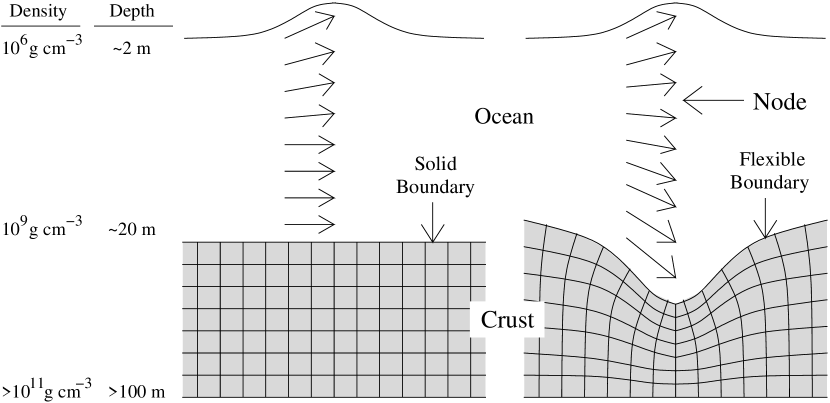
Figure 1.— A schematic diagram of an ocean surface wave showing how it is altered by the flexing of the crust. The vectors show the wave velocity. In both cases the transverse velocity is approximately constant within the ocean and dies off quickly into the crust. If the crust is treated as if it is “solid” the radial displacement goes to zero at the ocean floor (left diagram). As shown on the right, the interface mode has a large, negative radial displacement at the crust which is actually larger than the corresponding swell near the ocean surface. This implies that its radial eigenfunction must necessarily have a single node within the ocean.

This simple picture describes the interface mode quite well. The frequency depends on the properties at the base of the ocean, like a surface ocean wave, but with a frequency that is altered by the non-zero radial displacement at the ocean/crust boundary. This boundary condition reduces the frequency by $\sim(\mu/P)^{1/2}\sim 0.1$ from what is expected if the crust were “solid,” where $\mu$ is the shear modulus and $P$ is the pressure at the top of the crust. Most of the energy of the mode is in the ocean, just as in a shallow surface wave.

We derive the adiabatic perturbation equations for a plane parallel layer in hydrostatic balance with a shear stress in §2. These are used in §3 to analytically estimate the interface mode’s radial eigenfunction and frequency. We follow this with a numerical study in §4 that confirms our analytic results and also provides more detail about the eigenfunctions. We conclude in §5 with a discussion of possible uses for the interface mode in astrophysical contexts. Maybe most exciting among these is an additional mode of oscillation in WDs with crystalline cores.

2. Adiabatic Perturbation Equations

Since the pressure scale height in the NS ocean, $h=P/(\rho g)\approx(2-10)\times 10^{2}\textrm{ cm}$, is always much less the NS radius, $R\approx 10^{6}\textrm{ cm}$, we approximate the surface as having constant gravitational acceleration, $g=GM/R^{2}$ (neglecting general relativity), and plane parallel geometry. We use $z$ as our radial coordinate and $x$ as the transverse coordinate. An additional useful coordinate in this geometry is the column depth, denoted as $y$ (defined by $dy=-\rho dz$ and with cgs units of $\textrm{ g cm}^{-2}$).

The interface mode’s period is set by physics at the ocean/crust boundary, and is insensitive to the outer boundary condition. At these depths the thermal timescale is longer than the mode period (since $t_{\rm th}\approx c_{p}yT/F$ and $y$ is large; where $c_{p}$ is the specific heat capacity and $F$ is the flux) so that the perturbations are adiabatic. The governing equations of the envelope are conservation of mass, $\partial\rho/\partial t+\mbox{\boldmath$\nabla$}\cdot(\rho{\bf v})=0$, and momentum,

$$\rho\left(\frac{\partial}{\partial t}+v_{j}\frac{\partial}{\partial x_{j}}\right)v_{i}=\frac{\partial}{\partial x_{j}}\sigma_{ij}-\rho g\hat{\bf z},$$ (1)

where $\sigma_{ij}$ is the stress tensor, and $\hat{\bf z}$ is a radial unit vector (repeated indices imply the Einstein summation convention unless noted otherwise). We neglect the NS spin so that we can focus on the effects of the crust. Rotation can be simply included using the “traditional approximation” (e.g. Bildsten, Ushomirsky & Cutler 1996).

We make Eulerian perturbations of the conservation equations, substituting for the dependent variables $Q\rightarrow Q_{0}+\delta Q$, where $Q_{0}$ denotes the static background (this subscript is dropped in subsequent expressions). Perturbations are assumed to have the form $\delta Q=\delta Q(z)\exp(ik_{x}x+i\omega t)$, where $k_{x}^{2}=l(l+1)/R^{2}$ is the transverse wavenumber and $\omega$ is the mode frequency. These Eulerian perturbations are related to Lagrangian perturbations by $\Delta Q=\delta Q+\mbox{\boldmath$\xi$}\cdot\mbox{\boldmath$\nabla$}Q$. Since the background model has no fluid motion we substitute ${\bf v}\rightarrow\delta{\bf v}=d\mbox{\boldmath$\xi$}/dt=i\omega\mbox{\boldmath$\xi$}$, where $\xi$ is the local Lagrangian displacement. We use the Cowling approximation and neglect perturbations of the gravitational potential (Cowling 1941), an excellent approximation in the thin outer layers of the NS. Keeping terms of linear order, we find

$$\delta\rho+\mbox{\boldmath$\nabla$}\cdot(\rho\mbox{\boldmath$\xi$})=0,$$ (2)

for continuity.

In making linear perturbations of equation (1) we include the effects of a finite shear modulus (such as in the NS crust). Relative displacements then introduce a shear component to the Lagrangian stress tensor given by (Landau & Lifshitz 1970).

$$\Delta\sigma^{s}_{ij}=\mu\left(\frac{\partial\xi_{i}}{\partial x_{j}}+\frac{\partial\xi_{j}}{\partial x_{i}}-\frac{2}{3}(\mbox{\boldmath$\nabla$}\cdot\mbox{\boldmath$\xi$})\delta_{ij}\right),$$ (3)

where $\mu$ is the crystalline shear modulus as calculated by Strohmayer et al. (1991) for a classical one-component plasma (OCP),

$$\mu=\frac{0.1194}{1+0.595(173/\Gamma)^{2}}\frac{n_{i}(Ze)^{2}}{a},$$ (4)

where $n_{i}$ is the ion number density, $a=(3/4\pi n_{i})^{1/3}$ is the average ion spacing, $Z$ is the charge per ion, and

$$\Gamma\equiv\frac{(Ze)^{2}}{ak_{\rm B}T}=\frac{127}{T_{8}/4}\left(\frac{Z}{30}\right)^{2}\left(\frac{64}{A}\right)^{1/3}\left(\frac{\rho}{10^{9}\textrm{ g cm}^{-3}}\right)^{1/3},$$ (5)

is the dimensionless parameter that determines the liquid/solid transition for the OCP, where $k_{\rm B}$ is Boltzmann’s constant, $T_{8}\equiv T/10^{8}\textrm{ K}$, and $A$ is the number of nucleons per ion. This transition occurs at $\Gamma\approx 173$ (Farouki & Hamaguchi 1993 and references therein, following the work of Brush, Sahkin & Teller 1966). Since the pressure in the crust is dominated by degenerate electrons we rewrite $\mu$ as

$$\frac{\mu}{P}=\frac{1.4\times 10^{-2}}{1+0.595(173/\Gamma)^{2}}\left(\frac{Z}{30}\right)^{2/3}.$$ (6)

In the crust $\mu/P$ is fairly independent of temperature (except for a small dependence due to the factor of $\Gamma$ in the denominator), so we typically substitute $\mu_{0}\equiv\mu/P$ and assume that $\mu_{0}$ is constant with depth.

In the adiabatic limit, $\Delta P/P=\Delta\rho/(\Gamma_{1}\rho)$, where $\Gamma_{1}\equiv(\partial\ln P/\partial\ln\rho)_{s}$ is the adiabatic exponent. The Lagrangian stress tensor is

$$\Delta\sigma_{ij}=P\Gamma_{1}(\mbox{\boldmath$\nabla$}\cdot\mbox{\boldmath$\xi$})\delta_{ij}+\Delta\sigma^{s}_{ij},$$ (7)

and the Eulerian stress tensor is

$$\delta\sigma_{ij}=\Delta\sigma_{ij}-\rho g\xi_{z}\delta_{ij},$$ (8)

so that the perturbed momentum balance equation is

$$-\rho\omega^{2}\xi_{i}=\frac{\partial}{\partial x_{j}}\delta\sigma_{ij}-\delta\rho g\hat{\bf z}.$$ (9)

Equations (2) and (9) describe the nonradial oscillations.

The fluid viscosity in the ocean barely resists shear so that the Lagrangian stress tensor has only diagonal components, $\Delta\sigma_{ij}=-\Delta P\delta_{ij}$. Breaking equation (9) into radial and transverse components,

$$-\rho\omega^{2}\xi_{z} = -\frac{d\delta P}{dz}-g\delta\rho,$$ (10)

$$-\rho\omega^{2}\xi_{x} = -ik\delta P.$$ (11)

Combining equations (2), (10), and (11) results in the standard nonradial oscillation equations for an inviscid fluid in hydrostatic balance and plane parallel geometry,

$$\frac{d\xi_{z}}{dz}-\frac{\xi_{z}}{\Gamma_{1}h}=\left(\frac{ghk_{x}^{2}}{\omega^{2}}-\frac{1}{\Gamma_{1}}\right)\frac{\delta P}{P},$$ (12)

$$\frac{d}{dz}\frac{\delta P}{P}-\left(1-\frac{1}{\Gamma_{1}}\right)\frac{1}{h}\frac{\delta P}{P}=\left(\frac{\omega^{2}}{g}-\frac{N^{2}}{g}\right)\frac{\xi_{z}}{h},$$ (13)

where

$$N^{2}=-g\left(\frac{d\log\rho}{dz}-\frac{1}{\Gamma_{1}}\frac{d\log P}{dz}\right),$$ (14)

is the Brunt-Väisälä frequency which measures the internal buoyancy of the envelope. Normal modes of oscillation are found by assuming $\Delta P=0$ at the top boundary (a fluid element riding at the top feels no pressure perturbation) and then shooting for the bottom boundary condition. This top condition, though not unique, is fairly robust since little mode energy resides in the low density upper altitudes of the ocean (BC95).

When $\mu\neq 0$, expanding equation (9) in both the radial and transverse directions, and using the adiabatic condition and equation (2) to eliminate $\delta\rho$ and $\delta P$, results in

$$-\frac{d^{2}\xi_{z}}{dz^{2}}\left(\Gamma_{1}+\frac{4\mu}{3P}\right) = \xi_{z}\left(\frac{\omega^{2}}{gh}-\frac{\mu k_{x}^{2}}{P}\right)$$ (15)

$$+\frac{d\xi_{z}}{dz}\left(\frac{4}{3P}\frac{d\mu}{dz}-\frac{\Gamma_{1}}{h}+\frac{d\Gamma_{1}}{dz}\right)$$

$$+ik_{x}\xi_{x}\left[\frac{(1-\Gamma_{1})}{h}-\frac{2}{3P}\frac{d\mu}{dz}+\frac{d\Gamma_{1}}{dz}\right]$$

$$+ik_{x}\frac{d\xi_{x}}{dz}\left(\frac{\mu}{3P}+\Gamma_{1}\right),$$

and

$$-\frac{\mu}{P}\frac{d^{2}\xi_{x}}{dz^{2}} = \xi_{x}\left(\frac{\omega^{2}}{gh}-\frac{4k_{x}^{2}\mu}{3P}-\Gamma_{1}k_{x}^{2}\right)+\frac{1}{P}\frac{d\mu}{dz}\frac{d\xi_{x}}{dz}$$ (16)

$$+ik_{x}\xi_{z}\left(\frac{1}{P}\frac{d\mu}{dz}-\frac{1}{h}\right)+ik_{x}\frac{d\xi_{z}}{dz}\left(\frac{\mu}{3P}+\Gamma_{1}\right),$$

the crustal mode equations derived by BC95.

The second derivatives in equations (15) and (16) imply additional boundary conditions at the ocean/crust interface. We require that $\xi_{z}$ is continuous, so that there is no “space” between the two layers, and that $\Delta\sigma_{zz}$ is continuous, otherwise there is an infinite radial acceleration across the boundary. Furthermore, $\Delta\sigma_{xz}=0$ because the ocean, with no shear modulus, cannot sustain finite transverse shear. We also require the additional boundary conditions that $\xi_{z}\approx\xi_{x}\approx 0$ at some depth deep within the crust. Though this is not necessarily the case, it is helpful for estimating the interface mode’s frequencies.

3. Analytic Estimates

We now use these differential equations to analytically derive the frequencies and eigenfunctions of the interface mode. As we explain in Appendix A, the interface wave is not well described by WKB analysis, so we proceed with use of analogies to shallow ocean surface waves. In §3.1, we solve equations (12) and (13) for a surface wave, and consider how its frequency changes when $\xi_{z}\neq 0$ at the ocean floor (as suggested by Figure 1). In §3.2 we solve for the radial crustal eigenfunction, which we use in $\S 3.3$ to connect to the ocean perturbation and find the radial displacement at the interface. In §3.4 we summarize our frequency prediction for the interface wave and show how it depends on the temperature and composition of the NS crust.

3.1. Surface Wave Analytics

We assume that the surface wave in the ocean has a constant transverse displacement so that $\xi_{x}=\xi_{x,\rm t}$ and $d\xi/dz=0$ (where we use the subscript “t” to denote the “top” of the ocean). At the top the boundary condition is $\Delta P=0=\delta P-\xi_{z}\rho g$, and by combining this with transverse momentum conservation, equation (11), we relate the surface radial and transverse displacements

$$\xi_{z,\rm t}=\frac{\omega^{2}}{ikg}\xi_{x,\rm t}.$$ (17)

Using equation (11) to eliminate $\delta P$ from equation (12), and then eliminating $\xi_{x,\rm t}$ using equation (17),

$$\frac{d\xi_{z}}{dz}-\frac{\xi_{z}}{\Gamma_{1}h}=\frac{\xi_{z,\rm t}}{h}\left(\frac{ghk_{x}^{2}}{\omega^{2}}-\frac{1}{\Gamma_{1}}\right).$$ (18)

The electrons in the deep NS ocean are degenerate and relativistic so that the equation of state can be approximated by a $P=K\rho^{4/3}$ polytrope, where $K$ is a function of the mean molecular weight per electron. Using hydrostatic balance, the pressure scale height is

$$h(z)=\frac{1}{4}(z_{\rm t}-z),$$ (19)

where $z_{\rm t}\equiv 4K\rho^{1/3}_{\rm c}/g$, the subscript “c” denotes the top of the “crust”, and $z=0$ at the ocean/crust interface (we also make the approximation that $\rho_{\rm c}\gg\rho_{\rm t}$). Substituting this for $h$ in equation (18) and integrating gives,

$$\frac{\xi_{z}(z)}{\xi_{z,\rm t}}=1-\left(\frac{4}{\Gamma_{1}}+1\right)^{-1}\frac{gk_{x}^{2}}{\omega^{2}}\left(z_{\rm t}-z\right),$$ (20)

where the constant of integration is set to assure that $\xi_{z}=\xi_{z,\rm t}$ at $z=z_{\rm t}$.

The frequency of this surface wave is set by specifying the boundary condition $\xi_{z,\rm c}\equiv\xi_{z}(z=0)$. Substituting this into equation (20) we find a frequency

$$\omega^{2}=\frac{(4/\Gamma_{1}+1)^{-1}gk_{x}^{2}z_{\rm t}}{1-\xi_{z,\rm c}/\xi_{z,\rm t}}.$$ (21)

To understand this result it is helpful to compare it to the frequency for a mode with $\xi_{z,\rm c}=0$ as expected for a solid floor, which we denote as $\omega_{0}$. This results in

$$\omega^{2}_{0}=\left(\frac{4}{\Gamma_{1}}+1\right)^{-1}gk_{x}^{2}z_{\rm t}.$$ (22)

For $\Gamma_{1}=4/3$ we find that $\omega^{2}_{0}=gh_{\rm c}k_{x}^{2}$, where $h_{\rm c}$ is the scale height at the bottom of the ocean, just as expected for the shallow surface wave. The interface mode’s frequency is then

$$\omega^{2}=\omega^{2}_{0}/(1-\xi_{z,\rm c}/\xi_{z,\rm t}).$$ (23)

We expect $\xi_{z,\rm c}/\xi_{z,\rm t}<0$ because a positive pressure perturbation will compress the crust (see the discussion in §1 and Figure 1). Equation (23) shows that flexing of the crust results in a lower frequency than what would be expected if the ocean floor were solid.

3.2. The Radial Crustal Eigenfunction

To simplify equations (15), so that it can be solved analytically, we order the terms and drop those which are small. We first relate the ordering of the transverse and radial displacements within the crust. The ocean and crust slip with respect to one another so that the transverse displacement changes discontinuously at the boundary. We therefore set $\xi_{x,\rm c}=\lambda\xi_{x,\rm t}$ where $\lambda$ is a dimensionless constant which we call the “discontinuity eigenvalue.” It determines how $\xi_{x}$ changes at the interface, and is an eigenvalue set by the bottom boundary condition within the crust. We then rewrite equation (17) as

$$\xi_{x,\rm c}=\frac{igk_{x}}{\omega^{2}}\lambda\xi_{z,\rm t}.$$ (24)

At the top of the crust, the displacements must satisfy $\Delta\sigma_{xz}=0$ so that

$$\mu_{0}\frac{d\xi_{z}}{dz}+\mu_{0}ik_{x}\xi_{z}=0,$$ (25)

where we have used $\mu_{0}\equiv\mu/P$. Assuming that $\mathcal{O}(d\xi_{x}/dz)\sim\mathcal{O}(\xi_{x,\rm c}/h)$ within the crust, we combine equations (24) and (25) to find

$$\mathcal{O}(\lambda)\sim\mathcal{O}\left(\frac{\omega^{2}h}{g}\frac{\xi_{z}}{\xi_{z,\rm t}}\right).$$ (26)

The largest reasonable frequency is that of a discontinuity g-mode at the boundary ($\omega^{2}\approx ghk_{x}^{2}$) for which the terms in equation (15) with $\omega^{2}$ appearing are negligible. Using order of magnitude estimates of $k_{x}h\sim 10^{-4}-10^{-3}$ and $\mu_{0}\approx 10^{-2}$, from equation (6), we identify the two highest order terms of equation (15), resulting in

$$\frac{d^{2}\xi_{z}}{dz^{2}}=\frac{1}{h}\frac{d\xi_{z}}{dz},$$ (27)

as the simplified radial differential equation.

Since $\Gamma_{1}\approx 4/3$, we introduce a new radial variable, $s$, defined by $s=4h$ which is set equal to $s_{\rm c}$ at the ocean/crust interface and increases going down so that $ds=-dz$. Integration of equation (27) results in two constants of integration. The first is set by requiring that $\xi_{z}=\xi_{z,\rm c}$ at $s=s_{\rm c}$ and the second by requiring that $\xi_{z}=0$ at some bottom depth, which we denote as $s_{\rm b}$, so that

$$\xi_{z}(s)=\xi_{z,\rm c}\left[\frac{\left(s_{\rm b}/s\right)^{3}-1}{\left(s_{\rm b}/s_{\rm c}\right)^{3}-1}\right].$$ (28)

If we place the lower boundary condition infinitely deep within the crust, so that $s_{\rm b}\gg s_{\rm c}$, equation (28) simplifies to

$$\xi_{z}(s)=\xi_{z,\rm c}\left(s_{\rm c}/s\right)^{3},$$ (29)

identical to what BC95 estimate for the crustal eigenfunction (in their case in the context of a g-mode extending into the crust).

3.3. Connecting the Modes at the Ocean/Crust Boundary

We solve for $\xi_{z,\rm c}$, and estimate the mode frequency using equation (21), by demanding that $\Delta\sigma_{zz}$ be continuous across the ocean/crust boundary to avoid infinite radial accelerations. Expanding this component of the stress tensor,

$$\frac{\Delta\sigma_{zz}}{P}=\left(\Gamma_{1}-\frac{2\mu_{0}}{3}\right)\left(\mbox{\boldmath$\nabla$}\cdot\mbox{\boldmath$\xi$}\right)+2\mu_{0}\frac{d\xi_{z}}{dz}.$$ (30)

We evaluate this condition using the eigenfunctions we have found for both the ocean and crust. In the ocean, above the interface,

$$\left(\frac{\Delta\sigma_{zz}}{P}\right)_{\rm above}=\frac{1}{h_{\rm c}}(\xi_{z,\rm c}-\xi_{z,\rm t}).$$ (31)

In the crust we use equation (28) to evaluate $d\xi_{z}/dz$. The term involving $ik_{x}\xi_{x}$ can be ignored because it is order $(k_{x}h_{\rm c})^{2}$ less than the $d\xi_{z}/dz$ term (see Appendix B), so that below the interface,

$$\left(\frac{\Delta\sigma_{zz}}{P}\right)_{\rm below}\approx\left(\frac{3\Gamma_{1}/4+\mu_{0}}{1-(s_{\rm c}/s_{\rm b})^{3}}\right)\frac{\xi_{z,\rm c}}{h_{\rm c}},$$ (32)

where we have substituted $s_{\rm c}=4h_{\rm c}$. Setting equations (31) and (32) equal, we solve for the radial displacement at the crust,

$$\frac{\xi_{z,\rm c}}{\xi_{z,\rm t}}=-\left[\frac{3\Gamma_{1}/4+\mu_{0}}{1-(s_{\rm c}/s_{\rm b})^{3}}-1\right]^{-1}\approx-\frac{1}{\mu_{0}},$$ (33)

where the last estimate is made for $\Gamma_{1}=4/3$ and $s_{\rm b}\gg s_{\rm c}$.

3.4. Interface Wave Frequency Estimate

From our estimate for the eigenfrequency, equation (23), along with $\xi_{z,\rm c}/\xi_{z,\rm t}\approx-1/\mu_{0}$, equation (33), we find the simple result that

$$\omega^{2}\approx\mu_{0}\omega_{0}^{2},$$ (34)

The frequency of the interface mode is a factor of $\mu_{0}^{1/2}\sim 0.1$ less than a shallow surface wave in the NS ocean.

It is an interesting exercise to use this result to predict the interface wave’s frequency and dependence on the ocean/crust boundary’s properties. At this depth, the pressure is dominated by relativistic and degenerate electrons with a Fermi energy of ($E_{\rm F}\gtrsim m_{e}c^{2}\gg k_{\rm B}T$)

$$E_{\rm F}=4.1\textrm{ MeV}\left(\frac{2Z}{A}\right)^{1/3}\left(\frac{\rho}{10^{9}\textrm{g cm}^{-3}}\right)^{1/3}.$$ (35)

Since the pressure is $P\approx n_{e}E_{\rm F}/4$, the scale height at the crust is

$$h_{\rm c}=2620\textrm{ cm}\left(\frac{2Z}{A}\right)^{4/3}\left(\frac{\rho}{10^{9}\textrm{g cm}^{-3}}\right)^{1/3}.$$ (36)

Using $\omega_{0}=gh_{\rm c}k_{x}^{2}$ and substituting $\Gamma$ from equation (5) to eliminate $\rho$, we find the interface wave has a frequency of

$$\frac{\omega}{2\pi} \approx 16.5\textrm{ Hz}\left(\frac{\Gamma}{173}\right)^{1/2}\left(\frac{T_{8}}{4}\right)^{1/2}$$ (37)

$$\times\left(\frac{64}{A}\right)^{1/2}\left(\frac{10\textrm{ km}}{R}\right)\left[\frac{l(l+1)}{2}\right]^{1/2}.$$

For an accreting NS with a relatively cold ocean (similar to BC95 or what we consider in §4.1), this frequency is between the g-mode frequencies, $\lesssim 6\textrm{ Hz}$ (BC95), and the f-mode frequency, $\sim 10^{3}\textrm{ Hz}$, an otherwise empty part of the frequency domain. Furthermore, the interface mode frequency is independent of $Z$ and has a simple scaling with both $A$ and $T$, making this mode a useful diagnostic for measuring the properties of the NS crust.

4. Numerical Solutions

We now compute eigenfunctions and frequencies for the interface mode using numerical integrations of the mode equations on a two-component, ocean/crust NS model. In §4.2 we show that these compare very well with the analytic work of §3.

4.1. NS Ocean and Crust

We assume that the NS has a mass of $M=1.4M_{\odot}$ and radius of $R=10\textrm{ km}$. The two components which make up our NS envelope are a liquid ocean and a degenerate crystalline crust (see Figure 1). For accreting NSs, the composition of each of these components is determined by nuclear burning processes which occur on the surface, especially the rp-process during type I X-rays bursts (Wallace & Woosely 1981; Schatz et al. 1999, 2002) and the hotter burning during superbursts (Cumming & Bildsten 2001; Schatz, Bildsten & Cumming 2003). Woosley et al. (2004) follow the accretion and subsequent unstable burning over multiple type I bursts in numerical simulations. Estimating their results for an accreted composition of 0.05 solar metallicity and an accretion rate of $1.75\times 10^{-9}M_{\odot}\textrm{ yr}^{-1}$ (which they denote model “zM”) after 14 bursts, we assume a composition with mass fractions of ⁶⁴Zn(0.56), ⁶⁸Ge(0.35), ¹⁰⁴Pd(0.07) and ¹⁰⁶Cd(0.02), for both the ocean and crust. At sufficient pressure and density, this material will change from liquid to solid. This transition occurs at $\Gamma\approx 173$ (see §2.1) which implies a critical density of

$$\rho_{\rm c} = 2.5\times 10^{9}\textrm{ g cm}^{-3}\left(\frac{T_{8}}{4}\right)^{3}$$ (38)

$$\times\left(\frac{A}{64}\right)\left(\frac{30}{Z}\right)^{6}\left(\frac{\Gamma}{173}\right)^{3},$$

for an OCP. We assume that this is a good enough approximation even though we use a multi-component composition. Due to the strong dependence of this critical density on $Z$, in cases where burning results in ashes of especially heavy elements (such as the rp-process at high accretion rates or during superbursts) crystallization can happen at significantly shallower depths. This decreases the energy needed for large mode amplitudes.

The envelope profile is described by the equation of radiative transfer, which after substituting $y$ is

$$F=\frac{4acT^{3}}{3\kappa}\frac{dT}{dy},$$ (39)

where $a$ is the radiation constant and $\kappa$ is the opacity. The opacity is set using electron-scattering (Paczyński 1983), free-free (Clayton 1993 with the Gaunt factor of Schatz et al. 1999), and conductive opacities (Schatz et al. 1999 using the basic form of Yakovlev & Urpin 1980) in the liquid region. In the crust we make no distinction and use the same conductive opacity.

Equation (39) is integrated starting at an outer column depth ($y\approx 10^{7}\textrm{ g cm}^{-2}$) and into the envelope. The outer temperature is set near $10^{8}\textrm{ K}$, a value for which the solutions are minimally sensitive because of their radiative zero nature (Schwarzschild 1958, or see the discussion in Piro & Bildsten 2004). Previous studies of constantly accreting NSs have shown that the interior thermal balance is set by electron captures, neutron emissions, and pycnonuclear reaction in the inner crust (Miralda-Escudé, Paczyński & Haensel 1990; Bildsten & Brown 1997; Brown & Bildsten 1998) which release $\approx 1\textrm{ MeV}/m_{p}\approx 10^{18}\textrm{ erg g}^{-1}$ (Haensel & Zudunik 1990). Depending on the accretion rate and thermal structure of the crust, this energy will either be conducted into the core or released into the ocean such that for an Eddington accretion rate up to $\approx 92\%$ of the energy is lost to the core and exists as neutrinos (Brown 2000). We therefore set the flux in the ocean to a fiducial value of $10^{21}\textrm{ erg s}^{-1}\textrm{cm}^{-2}$ (as expected for an accretion rate of $\sim 10^{-9}M_{\odot}\textrm{ yr}^{-1}$, about one-tenth the Eddington rate). We solve for $\rho$ using the analytic equation of state from Paczyński (1983) which is applicable to both the ocean and crust. The profiles are continuous across the ocean/crust interface because we assume the same conductive opacity in each region. Figure 2 shows the envelope profile for the variables most important for determining the mode properties. The dashed line denotes the location of the crust (which we assume is at a column depth of $y_{\rm c}=10^{13}\textrm{ g cm}^{-2}$, near a density of $\rho_{\rm c}\approx 10^{9}\textrm{ g cm}^{-3}$).

Figure 2.— Temperature, density, and Brunt-Väisälä frequency for our two-component neutron star envelope. The dashed line denotes the depth of the ocean/crust boundary, which lacks a discontinuity because we use the same conductive opacity in each region. The flux is assumed to be constant at $F=10^{21}\textrm{ erg s}^{-1}\textrm{ cm}^{-2}$ with no other heat sources. This is a fiducial value expected for accreting neutron stars which have their internal thermal balance set by electron captures, neutron emissions, and pycnonuclear reactions in the inner crust. These reactions release $\approx 1\textrm{ MeV}/m_{p}$ with typically $\approx 0.1\textrm{ MeV}/m_{p}$ making its way into the upper crust (Brown 2000). The power law of the density ($\rho\propto y^{3/4}$) shows that the pressure in the crust is set by degenerate, relativistic electrons.

4.2. Numerical Integrations and Comparisons with Analytics

Using the envelope profile of §4.1, we numerically solve for the interface wave eigenfunctions and eigenfrequencies. We treat each integration as a two eigenvalue shooting problem, first choosing $\omega$ and $\lambda$ and then shooting for the bottom boundary condition. We integrate equations (12) and (13), beginning at the top of the ocean at a column of $y_{\rm t}\approx 10^{8}\textrm{ g cm}^{-2}$ (where the unstable burning of X-ray bursts typically occurs; Bildsten 1998) where we set $\Delta P=0$. The boundary conditions at the ocean/crust interface are set by requiring $\xi_{z}$ to be continuous, $\Delta\sigma_{xz}=0$ (which sets $d\xi_{x}/dz$), and $\Delta\sigma_{zz}$ continuous across the boundary (which sets $d\xi_{z}/dz$). The discontinuity of $\xi_{x}$ is set using $\lambda$. We then integrate equations (15) and (16) into the NS crust (we assume that $d\mu_{0}/dz\approx d\Gamma_{1}/dz\approx 0$ and simply set $\mu_{0}=10^{-2}$ for these examples) down to a depth within the crust where we require both $\xi_{x}$ and $\xi_{z}$ to be zero. We leave the bottom boundary depth as a free parameter and study how the eigenvalues and eigenfunctions change with this variable.

In Figure 3 we show example eigenfunctions with a bottom boundary at $y_{\rm b}=10^{16}\textrm{ g cm}^{-2}$. On the same plot we also compare the analytic eigenfunctions from §3.2 and Appendix B. These use the numeric envelope model to set the local scale height and $\Gamma_{1}=1.338$ (its value at the ocean/crust boundary) to set the eigenvalues. The numerical eigenvalues are $\omega/(2\pi)=23.43.\textrm{ Hz}$ and $\lambda=-1.5\times 10^{-4}$, which are close to the analytic values of $\omega/(2\pi)=24.46\textrm{ Hz}$ and $\lambda=-1.8\times 10^{-4}$. As shown in Figure 1, the radial displacement is found to be very large at the interface, relative to its value at the ocean surface. The energy density (per logarithm of pressure) is

$$\frac{dE}{d\log y}=\frac{1}{2}4\pi R^{2}\omega^{2}\xi^{2}y,$$ (40)

where $\xi^{2}=|\xi_{x}|^{2}+|\xi_{z}|^{2}$, which shows where the mode “lives.” The energy density is also strongly concentrated at the interface, consistent with the result that the mode’s properties are set by the envelope at this depth.

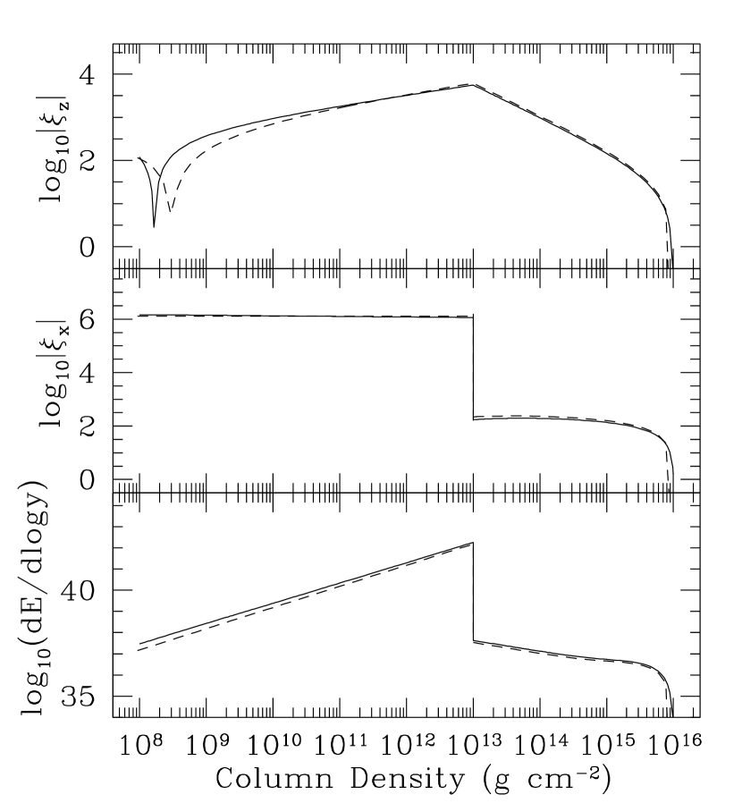
Figure 3.— A comparison of the numerical eigenfunctions (solid curves) and the analytic approximations (dashed lines) for the interface mode using the envelope shown in Figure 2, with the bottom boundary set at $y_{\rm b}=10^{16}\textrm{ g cm}^{-2}$. The numerical solutions find $\omega/(2\pi)=23.43\textrm{ Hz}$ and $\lambda=-1.5\times 10^{-4}$, while the analytic values are $\omega/(2\pi)=24.46\textrm{ Hz}$ and $\lambda=-1.8\times 10^{-4}$, using equations (21) and (B7), respectively. The analytic solutions use the numeric envelope to set the local scale height, and $\Gamma_{1}=1.369$ to set the eigenvalues (this is the value of $\Gamma_{1}$ at the base of the ocean). The radial eigenfunction, $\xi_{z}$, shows a single node in the ocean and a large displacement at the crust ($y_{\rm c}=10^{13}\textrm{ g cm}^{-2}$), consistent with the discussion in §1. The energy density (bottom panel) shows that the mode energy is concentrated in the ocean.

As a comparison, we plot $\xi_{z}$ for both the correct and the “solid” ocean/crustal boundary conditions in Figure 4. For the latter we find a frequency of $\omega_{0}/(2\pi)=179.62\textrm{ Hz}$. The linear plot of the amplitudes shows how extreme the radial displacement is at the crust for the interface mode. We omit comparing $\xi_{x}$ and the energy density for the modes since they are almost identical in the ocean.

Figure 4.— A comparison of the $\xi_{z}$ eigenfunction between a correctly calculated interface wave (solid curve) and the case of when the crustal boundary is set to $\xi_{z}=0$ (a standard shallow ocean wave; dashed curve). The latter case has an eigenfrequency of $\omega_{0}/(2\pi)=179.62\textrm{ Hz}$ and no node in the ocean, in contrast to the interface wave’s eigenfrequency of $\omega/(2\pi)=23.43\textrm{ Hz}$. The linear plot of the displacements (bottom panel) emphasizes the large displacement at the boundary for the interface wave (note the other mode is magnified by a factor of 20).

To study the dependence of the mode’s properties on the bottom boundary condition within the crust, we compare the numeric and analytic results as a function of the bottom boundary depth, $y_{\rm b}$, in Figure 5. On the left hand side is the limit when there is no penetration into the crust, in this case both the ratio $\xi_{z,\rm c}/\xi_{z,\rm t}$ and $\lambda$ are zero and $\omega/(2\pi)\sim 200\textrm{ Hz}$, the values which would be approximated for a shallow surface wave (see Figure 4). As the bottom boundary is set deeper, the frequency decreases, becoming nearly, but not quite equal to $\sim\mu_{0}^{1/2}\times 200\textrm{ Hz}\sim 20\textrm{ Hz}$.

Figure 5.— The properties of the interface mode as a function of the bottom boundary depth, using the envelope of Figure 2 with the crust at $y_{\rm c}=10^{13}\textrm{ g cm}^{-2}$. The solid curves show the analytic estimates, using equations (21), (B7) and (33) (from top to bottom), while the points mark the numerical calculations. On the far left we find what is expected for a shallow ocean wave, and as the curves move right (to larger depths) they become more like an interface wave.

5. Discussion and Conclusions

We have discussed the ocean/crust interface wave, investigating its properties both analytically and numerically for a two-component NS envelope. We show that it can be understood as a shallow surface wave, with a different radial displacement boundary condition at the bottom of the ocean. This reduces the frequency by roughly $\sim\mu_{0}^{1/2}\sim 0.1$ from what would be expected if the crust were instead “solid.” In general the interface wave is a global mode of oscillation, so that the entire star must be taken into account to calculate the mode to high precision (see discussion in Appendix C). Fortunately, by using our analysis, a fairly good estimate of the mode frequency can be made just from considering the NS properties right near the ocean/crust interface because the majority of mode energy ($\gtrsim 99\%$) resides in the NS ocean.

The interface wave should be included in future studies of nonradial oscillations on both accreting and bursting NSs. For a non-rotating NS this would result in frequencies of $\sim 10-20\textrm{ Hz}$ which would then be altered and split due to the NS spin (Bildsten, Ushomirsky & Cutler 1996). The observation of multiple mode periods would greatly assist our understanding of the NS crust. The g-modes are sensitive to the depth of the crust (since it provides a bottom boundary), while the interface wave is sensitive to both the depth and the value of the shear modulus. This provides information about the temperature and composition of the crust, which is determined by unstable nuclear burning processes (X-ray bursts and superbursts) that happen in the ocean.

Since the example considered in this work is a relatively “cool” envelope, the g-mode frequencies ($\lesssim 6\textrm{ Hz}$) are well separated from the interface wave frequency ($\sim 10-20\textrm{ Hz}$). On a bursting NS, which has temperatures in the upper atmosphere as high as $10^{9}\textrm{ K}$, at least one g-mode has a frequency higher than the interface wave. The interface wave would then have an additional node in its eigenfunction, due to the relation between g-mode frequency ordering and number of nodes, but its frequency would be unchanged as long as the ocean stays at a temperature of $\sim 4\times 10^{8}\textrm{ K}$ (since this is where the mode’s energy is concentrated). Woosley et al. (2004) show that the thermal wave during an X-ray burst does not penetrate deeply into the ocean, so that our estimates for the interface mode frequency still hold.

The other important astrophysical context where our work can be applied is for old and/or massive WDs that have crystalline cores. This may be seen in the pulsations of BPM 37093 (Kanaan et al. 1992), a high-mass ZZ Ceti star that should be considerably crystallized (Winget et al. 1997). There is also the exciting possibility that some of the pulsators discovered through the Sloan Digital Sky Survey (Mukadam et al. 2004) may be massive enough to be crystallized. Scaling equation (37) to the fiducial interior properties of a $\approx 1.1M_{\odot}$ WD, we find a crustal mode period of

$$P \approx 95\textrm{ s}\left(\frac{173}{\Gamma}\right)^{1/2}\left(\frac{10^{7}\textrm{ K}}{T}\right)^{1/2}$$ (41)

$$\times\left(\frac{A}{16}\right)^{1/2}\left(\frac{R}{5\times 10^{8}\textrm{ cm}}\right)\left[\frac{2}{l(l+1)}\right]^{1/2},$$

which for the $l=1$ mode is between the periods of the f-mode ($\sim 10-20\textrm{ s}$) and g-modes ($\gtrsim 300\textrm{ s}$). HV79 (and more recently Montgomery & Winget 1999) previously calculated the spectrum of g-modes and torsional modes expected for these stars, concentrating on the effects of crystallization. HV79 do not single out any one mode as a “crustal mode,” but in their crystallized models their lowest order g-mode (which they denote ${}_{-1}S_{l}$) matches many of the properties we identify as being characteristic of a crustal mode. This includes a large radial displacement at the crust and a nearly constant transverse displacement in the WD “ocean” (see Figures 1 and 2 of HV79). Furthermore, HV79 find the period of their ${}_{-1}S_{l}$ mode to be between the f-mode and the other g-mode periods, in confirmation of our above discussion.

We thank both Phil Arras and Omer Blaes for helpful discussions. We also thank the referee, Michael Montgomery, for pointing out the HV79 paper and its relevance to our work. This work was supported by the National Science Foundation under grants PHY99-07949 and AST02-05956, and by the Joint Institute for Nuclear Astrophysics through NSF grant PHY02-16783.

Appendix A Influence of a Finite Shear Modulus

The interface wave’s properties are set by how it is influenced by the finite shear modulus of the NS crust. Unlike g-modes, which see the crust as solid, the interface wave reacts to the crust as if it is a flexible and compressible surface. We now explain why each of these cases occur.

Using $\mu_{0}\equiv\mu/P$, and assuming that $d\mu_{0}/dz\approx d\Gamma_{1}/dz\approx 0$, equations (15) and (16) can be rewritten as

$$-\frac{d^{2}\xi_{z}}{dz^{2}}\left(\Gamma_{1}+\frac{4}{3}\mu_{0}\right) = \xi_{z}\left(\frac{\omega^{2}}{gh}-k_{x}^{2}\mu_{0}\right)-\frac{d\xi_{z}}{dz}\left(\frac{4}{3}\frac{\mu_{0}}{h}+\frac{\Gamma_{1}}{h}\right)$$ (A1)

$$+ik_{x}\xi_{x}\left[\frac{(1-\Gamma_{1})}{h}+\frac{2}{3}\frac{\mu_{0}}{h}\right]$$

$$+ik_{x}\frac{d\xi_{x}}{dz}\left(\frac{\mu_{0}}{3}+\Gamma_{1}\right),$$

and

$$-\mu_{0}\frac{d^{2}\xi_{x}}{dz^{2}} = \xi_{x}\left(\frac{\omega^{2}}{gh}-\frac{4}{3}k_{x}^{2}\mu_{0}-\Gamma_{1}k_{x}^{2}\right)-\frac{\mu_{0}}{h}\frac{d\xi_{x}}{dz}$$ (A2)

$$-ik_{x}\xi_{z}\left(\frac{\mu_{0}}{h}+\frac{1}{h}\right)+ik_{x}\frac{d\xi_{z}}{dz}\left(\frac{\mu_{0}}{3}+\Gamma_{1}\right).$$

The simplest analysis of these equations arises when perturbations scale like $\sim\exp(ik_{z}z)$ and dispersion relations are in the WKB limit (when the radial wavenumber $k_{z}\gg 1/h$). This results in toroidal and spheroidal modes with frequencies

$$\omega^{2}_{\rm shear} = \mu_{0}(P/\rho)k^{2},$$ (A3)

$$\omega^{2}_{\rm sound} = (\Gamma_{1}+4\mu_{0}/3)(P/\rho)k^{2},$$ (A4)

where $k^{2}=k^{2}_{x}+k^{2}_{z}$ is the total wavenumber. The first is a shear mode (with a frequency of $\sim 10^{2}-10^{3}\textrm{ Hz}$) and the second is a sound wave slightly modified by $4\mu_{0}/3$ ($\sim 10^{4}-10^{5}\textrm{ Hz}$). These imply that a g-mode with a frequency of $\lesssim 6\textrm{ Hz}$ (BC95) will be reflected at the interface because of the frequency mismatch. Unfortunately, this analysis cannot be extended to the interface mode because it has $k_{z}\lesssim 1/h$, in contradiction to the WKB limit.

To see that a mode with a constant transverse velocity (like the interface wave) is not excluded from the crust we compare the transverse momentum terms from equation (9). The shear modulus term has two pieces, the larger one is $d\delta\sigma_{xz}/dz\sim\mu d^{2}\xi_{x}/dz^{2}$. This term strongly affects the mode’s eigenfunctions when it is comparable to the transverse acceleration of the mode, $\rho\omega^{2}\xi_{x}$. Using $d/dz\sim k_{z}$ this implies a critical shear modulus of $\mu_{\rm crit}/P\sim\omega^{2}/(ghk_{z}^{2})$. In the case of g-modes $k_{z}\sim 1/h$ and $\omega^{2}\approx 4N^{2}(hk_{x})^{2}$ so that the critical modulus is (BC95)

$$\frac{\mu_{\rm crit}}{P}(\textrm{g-mode})\sim\frac{6l(l+1)}{Z}\frac{k_{\rm B}T}{E_{\rm F}}\left(\frac{h}{R}\right)^{2}.$$ (A5)

Substituting values near the ocean/crust interface for degenerate, relativistic electrons,

$$\frac{\mu_{\rm crit}}{P}(\textrm{g-mode})\sim 10^{-11}T_{8}^{2}l(l+1)\left(\frac{64}{A}\right)^{2}\left(\frac{30}{Z}\right)^{2/3}\left(\frac{\Gamma}{173}\right),$$ (A6)

which is clearly less than the value of $\mu/P$ from equation (6), implying that the g-modes will be excluded from the crust.

One the other hand, the interface wave has a constant transverse velocity so that $k_{z}\sim 1/R$. Using $\omega^{2}\approx\mu_{0}ghk^{2}_{x}$, the interface wave has a critical shear modulus of

$$\frac{\mu_{\rm crit}}{P}(\textrm{interface wave})\sim\mu_{0}l(l+1),$$ (A7)

which is just the actual shear modulus present at the boundary, so the wave must penetrate the crust. This shows that in the interface wave the transverse momentum is perfectly balanced by the shear stress, so that the ocean/crust boundary behaves like a flexible and compressible surface.

Appendix B Transverse Crustal Eigenfunction and Discontinuity Eigenvalue

To estimate the transverse crustal eigenfunction, we order the terms from equation (A2) and drop those which are small. Using equations (24) and (26) we first relate the ordering of the transverse and radial displacements within the curst. Dividing equation (A2) through by $\xi_{z}$, multiplying through by $h^{2}$ and using the above relations, the ordering of each of the terms are

$$\mathcal{O}(\mu_{0}k_{x}h) \sim \mathcal{O}(\omega^{2}h^{2}k_{x}/g)+\mathcal{O}(\mu_{0}k_{x}^{3}h^{3})+\mathcal{O}(k_{x}^{3}h^{3})+\mathcal{O}(k_{x}h)$$ (B1)

$$+\mathcal{O}(\mu_{0}k_{x}h)+\mathcal{O}(k_{x}h)+\mathcal{O}(\mu_{0}k_{x}h)+\mathcal{O}(k_{x}h).$$

The size of these quantities are approximated using $k_{x}h\sim 10^{-4}-10^{-3}$ and $\mu_{0}\approx 10^{-2}$. Just as with the radial equation considered in §3.2, the terms which contain $\omega^{2}$ are negligible (as is seen from considering $\omega^{2}$ anywhere in the range of $\sim\mu_{0}ghk_{x}^{2}-ghk_{x}^{2}$). To find a relation which includes $\xi_{x}$ we must consider both first- and second-order terms of equation (A2) to get

$$-\mu_{0}\frac{d^{2}\xi_{x}}{dz^{2}} = -\frac{\mu_{0}}{h}\frac{d\xi_{x}}{dz}-ik\xi_{z}\left(\frac{\mu_{0}}{h}+\frac{1}{h}\right)$$ (B2)

$$+ik\frac{d\xi_{z}}{dz}\left(\frac{\mu_{0}}{3}+\Gamma_{1}\right),$$

as a new simplified differential equation.

We substitute the eigenfunction for $\xi_{z}$, equation (28) into equation (B2) to solve for $\xi_{x}$. The two constants of integration are set by imposing that $\Delta\sigma_{xz}=0$ at the top of the crust and that $\xi_{x}$ (just like $\xi_{z}$) goes to zero at $s_{\rm b}$, so that

$$\xi_{x}(s)=\frac{ik_{x}s_{\rm b}\xi_{z,\rm c}}{(s_{\rm b}/s_{\rm c})^{3}-1}\left\{\alpha\left[\left(\frac{s_{\rm b}}{s}\right)^{3}-1\right]+\beta\left[\left(\frac{s_{\rm b}}{s}\right)^{2}-1\right]\right.$$

$$\left.+\gamma\left[1-\frac{s}{s_{\rm b}}\right]\right\},\hskip 8.5359pt$$ (B3)

where we have introduced dimensionless constants that only depend on the star,

$$\alpha \equiv \frac{2\mu_{0}+4-3\Gamma_{1}}{3\mu_{0}}\frac{s_{\rm c}}{s_{\rm b}}-\frac{1}{3\mu_{0}}\left(\frac{s_{\rm c}}{s_{\rm b}}\right)^{4},$$ (B4)

$$\beta \equiv -\frac{3\mu_{0}+4-3\Gamma_{1}}{2\mu_{0}},$$ (B5)

$$\gamma \equiv 1+\frac{1}{\mu_{0}}.$$ (B6)

Substituting $s=s_{\rm c}$ and dividing by equation (17) we find

$$\lambda \equiv \frac{\xi_{x,\rm t}}{\xi_{x,\rm c}}$$ (B7)

$$= \frac{\omega^{2}s_{\rm b}/g}{(s_{\rm b}/s_{\rm c})^{3}-1}\frac{\xi_{z,\rm c}}{\xi_{z,\rm t}}\left\{\alpha\left[\left(\frac{s_{\rm b}}{s_{\rm c}}\right)^{3}-1\right]+\beta\left[\left(\frac{s_{\rm b}}{s_{\rm c}}\right)^{2}-1\right]\right.$$

$$\hskip 133.72786pt\left.+\gamma\left[1-\frac{s_{\rm c}}{s_{\rm b}}\right]\right\},$$

for the discontinuity eigenvalue.

We use equation (B3) (or consider the infinite crust limit of Appendix C), to see that the size of $\xi_{x,\rm c}/\xi_{z,\rm c}\sim k_{x}s_{\rm c}$. This shows that when we consider terms in equation (30), the $\xi_{x}$ terms are of order

$$\frac{k_{x}\xi_{x}}{d\xi_{z}/dz}\sim(k_{x}h_{\rm c})^{2}\ll 1,$$ (B8)

smaller than the $\xi_{z}$ terms and can thus be ignored.

Appendix C Infinite Crust Limit

Just as we did for the radial eigenfunction for equation (29), we take the $s_{\rm b}\gg s_{\rm c}$ limit on equation (B3) to find the transverse eigenfunctions in the infinite crust limit,

$$\xi_{x}(s) = ik_{x}s_{\rm c}\xi_{z,\rm c}\left[\frac{2\mu_{0}+4-3\Gamma_{1}}{3\mu_{0}}\left(\frac{s_{\rm c}}{s}\right)^{3}\right.\hskip 19.91684pt$$ (C1)

$$\hskip 42.67912pt\left.-\frac{3\mu_{0}+4-3\Gamma_{1}}{2\mu_{0}}\left(\frac{s_{\rm c}}{s}\right)^{2}\right],$$

$$\approx ik_{x}s_{\rm c}\xi_{z,\rm c}\left[\frac{2}{3}\left(\frac{s_{\rm c}}{s}\right)^{3}-\frac{3}{2}\left(\frac{s_{\rm c}}{s}\right)^{2}\right],$$

which corresponds to

$$\lambda = -\frac{\omega^{2}s_{\rm c}}{g}\frac{\xi_{z,\rm c}}{\xi_{z,\rm t}}\left(\frac{5\mu_{0}+4-3\Gamma_{1}}{6\mu_{0}}\right),$$ (C2)

$$\approx -\frac{5}{6}\frac{\omega^{2}s_{\rm c}}{g}\frac{\xi_{z,\rm c}}{\xi_{z,\rm t}},$$

for the discontinuity eigenvalue.

We use these eigenfunctions to estimate the mode’s energy density, $dE/d\log y$, from equation (37). We consider the limit of $s\rightarrow\infty$ to see if the energy density falls off with increasing depth. If this happens, it implies a natural depth at which to set a lower boundary and provides confidence that the interface mode is determined by conditions local to the ocean/crust boundary. Comparing equations (29) and (C1) we find that at depths of order the NS radius $\xi_{x}$ will dominate so that $\xi^{2}\propto 1/s^{4}$. For fully degenerate and relativistic material $P\propto y\propto\rho^{4/3}$. Using $h=P/(\rho g)$ and $h\propto s$ we find that $y\propto s^{4}$. This means that at the greatest possible depths $dE/d\log y\sim\xi^{2}y\sim\textrm{constant}$, so that, unfortunately, deep regions of the NS much be taken into account to calculate the interface mode to very high accuracy. In practice, this is not necessary because there are structural changes within a realistic NS crust that introduce new bottom boundaries. Due to the large amount of energy concentrated in the ocean ($\gtrsim 99\%$, see Figure 3), our frequency estimates are still good even with this difficulty.

References

- (1) Bildsten, L. 1998, in The Many Faces of Neutron Stars, ed. R. Buccheri, J. van Paradijs & A. Alpar (Dordrecht: Kluwer), 419
- (2) Bildsten, L. & Brown, E. F. 1997, ApJ, 477, 897
- (3) Bildsten, L. & Cumming, A. 1998, ApJ, 506, 842
- (4) Bildsten, L. & Cutler, C. 1995, ApJ, 449, 800 (BC95)
- (5) Bildsten, L., Ushomirsky, G. & Cutler, C. 1996, ApJ, 460, 827
- (6) Brown, E. F. 2000, ApJ, 531, 988
- (7) Brown, E. F. & Bildsten, L. 1998, ApJ, 496, 915
- (8) Brush, S. G., Sahlin, H. L. & Teller, E. 1966, J. Chem. Phys., 45, 2102
- (9) Clayton, D. D. 1983, Principles of Stellar Evolution and Nucleosynthesis (Chicago: Univ. Chicago Press)
- (10) Cowling, T. G. 1941, MNRAS, 101, 367
- (11) Cumming, A. & Bildsten, L. 2001, ApJ, 559, 127
- (12) Farouki, R. T. & Hamaguchi, S. 1993, Phys. Rev. E, 47, 4330
- (13) Finn, L. S. 1987, MNRAS, 227, 265
- (14) Haensel, P. & Zdunik, J. L. 1990, A&A, 227, 431
- (15) Hansen, C. J. & Van Horn, H. M. 1979, ApJ, 233, 253 (HV79)
- (16) Kanaan, A., Kepler, S. O., Giovannini, O. & Diaz, M. 1992, ApJ, 390, L89
- (17) McDermott, P. N. 1990, MNRAS, 245, 508
- (18) McDermott, P. N. & Taam, R. E. 1987, ApJ, 318, 278
- (19) McDermott, P. N., Van Horn, H. M. & Hansen, C. J. 1988, ApJ, 325, 725 (MVH88)
- (20) McDermott, P. N., Van Horn, H. M. & Scholl, J. F. 1983, ApJ, 268, 837
- (21) Miralda-Escudé, J., Paczyński, B. & Haensel, P. 1990, ApJ, 363, 572
- (22) Montgomery, M. H. & Winget, D. E. 1999, ApJ, 526, 976
- (23) Mukadam, A. S., et al. 2004, ApJ, 607, 982
- (24) Muno, M. P., Chakrabarty, D., Galloway, D. K. & Savov, P. 2001, ApJ, 553, L157
- (25) Paczyński, B. 1983, ApJ, 267, 315
- (26) Piro, A. L. & Bildsten, L. 2004, ApJ, 603, 252
- (27) Schatz, H., Bildsten, L. & Cumming, A. 2003, ApJ, 583, 87
- (28) Schatz, H., Bildsten, L., Cumming, A. & Wiescher, M. 1999, ApJ, 524, 1014
- (29) Schatz, H. et al. 2001, Phys. Rev. Lett., 86, 3471
- (30) Schwarzschild, M. 1958, Structure and Evolution of Stars (New York: Dover Publications)
- (31) Strohmayer, T. E. 1993, ApJ, 417, 273
- (32) Strohmayer, T. E. & Lee, U. 1996, ApJ, 467, 773
- (33) Strohmayer, T., Ogata, S., Iyetomi, H., Ichimaru, S. & Van Horn, H. M. 1991, ApJ, 375, 679
- (34) Wallace, R. K. & Woosley, S. E. 1981, ApJ, 45, 389
- (35) Winget, D. E., Kepler, S. O., Kanaan, A., Montgomery, M. H. & Giovannini, O. 1997, ApJ, 487, L191
- (36) Woosley, S. E. et al. 2004, ApJS, 151, 75
- (37) Yakovlev, D. G. & Urpin, V. A. 1980, Soviet Astron., 24, 303