Chemical enrichment of the complex hot ISM of the Antennae Galaxies: I. Spatial and spectral analysis of the diffuse X-ray emission

Abstract

We present an analysis of the properties of the hot interstellar medium (ISM) in the merging pair of galaxies known as The Antennae (NGC 4038/39), performed using the deep, coadded $\sim$411 ks Chandra ACIS-S data set. These deep X-ray observations and Chandra’s high angular resolution allow us to investigate the properties of the hot ISM with unprecedented spatial and spectral resolution. Through a spatially resolved spectral analysis, we find a variety of temperatures (from 0.2 to 0.7 keV) and $N_{H}$ (from Galactic to $2\times 10^{21}$ cm^-2). Metal abundances for Ne, Mg, Si, and Fe vary dramatically throughout the ISM from sub-solar values ($\sim$0.2) up to several times solar.

1 Introduction

The Antennae, dynamically modeled by Toomre & Toomre (1972) and Barnes (1988), are the nearest pair of colliding galaxies involved in a major merger (D = 19 Mpc for H${}_{o}=75~{}\rm km~{}s^{-1}~{}Mpc^{-1}$). Hence, this system provides a unique opportunity for getting the most detailed look possible at the consequences of a galaxy merger as evidenced by induced star formation and the conditions in the ISM. Each of the two colliding disks shows rings of giant H II regions and bright stellar knots with luminosities up to $M_{V}\sim-16$ (Rubin, Ford, & D’Odorico 1970), which are resolved with the Hubble Space Telescope (HST) into typically about a dozen young star clusters (Whitmore & Schweizer 1995; Whitmore et al. 1999). These knots coincide with the peaks of H$\alpha$, 2.2$\mu$, and 6-cm radio-continuum emission (Amram et al. 1992; Stanford et al. 1990; Neff & Ulvestad 2000), indicating an intensity of star formation in each single region exceeding that observed in 30 Doradus. CO aperture synthesis maps reveal major concentrations of molecular gas, including a $\sim$2.7$\times 10^{9}M_{\odot}$ concentration in the region where the two disks overlap (Stanford et al. 1990; Wilson et al. 2000). This concentration in the overlap region is coincident with the bright emission peaks seen in SCUBA 450$\mu$ and 850$\mu$ maps and ISOPHOT 60$\mu$ and 100$\mu$ observations (Haas et al. 2000), which show the simultaneous presence of warm dust ($T\approx 30$ K), usually observed in starbursts of luminous IR galaxies, and cold dust ($T<20$ K) more typical for quiet galaxies and extremely dense clouds. A K-band study derives ages for the star clusters ranging from 4 to 13 Myr, and yields high values of extinction ($A_{V}\sim 0.7-4.3$ mag; Mengel et al. 2000, 2005). Many of the youngest star clusters lie in the CO-rich overlap region, where even higher extinction is present ($A_{V}\lesssim 100$ mag), implying that they must lie in front of most of the gas (Wilson et al. 2003). Some of them are found as far as 2 kpc from detectable CO regions, leading to the conclusion that either they formed from clouds less massive than $5\times 10^{6}$ $M_{\odot}$ or they have already destroyed their parent molecular cloud, or perhaps both.

The presence of an abundant hot ISM in The Antennae was originally suggested by the first Einstein observations of this system (Fabbiano & Trinchieri 1983), and has since been confirmed with several major X-ray telescopes (ROSAT: Read, Ponman, & Wolstencroft 1995, Fabbiano, Schweizer, & Mackie 1997; and ASCA: Sansom et al. 1996). The ROSAT HRI image was used in a recent multiwavelength study of The Antennae by Zhang, Fall, & Whitmore (2001), which suggests feedback between star clusters and the interstellar medium (ISM). The first Chandra ACIS (Weisskopf, O’ Dell & van Speybroeck 1996) observation of The Antennae in 1999 (Fabbiano, Zezas & Murray 2001; Fabbiano et al. 2003, hereafter F03) gave us for the first time a detailed look at this hot ISM, revealing a complex, diffuse and soft emission component responsible for about half of the detected X-ray photons from the two merging galaxies. The spatial resolution of Chandra is at least 10 times superior to that of any other X-ray observatory, allowing us to resolve the emission on physical scales of $\sim$75 pc for D$=$19 Mpc, and to detect and subtract individual point-like sources (most likely X-ray binaries; see Zezas et al. 2002). At the same time, ACIS allows us to study for the first time the X-ray spectral properties of these emission regions, providing additional important constraints on their nature.

In the first detailed Chandra study of the hot ISM, F03, using the 1999 data, presented a “multi-color” X-ray image that suggests both extensive absorption by the dust in this system, peaking in the overlap region, as well as variations in the temperature of different emission regions of the hot ISM. These conclusions were confirmed by spectral fits to the data extracted from different regions, which suggested that at least two thermal components with temperatures of $\sim$0.3 and $\sim$0.7 keV are present in the luminous regions of the diffuse emission. The parameters derived for the hot ISM suggested that in the nuclear regions of the two colliding galaxies the mass of the hot ISM is $\sim$10⁵–10${}^{6}M_{\odot}$, much smaller than that in molecular gas (Wilson et al. 2000), but that the thermal pressures of the two phases of the ISM are comparable, suggesting equilibrium. Comparisons with H$\alpha$, radio-countinuum (Neff & Ulvestad 2000), and HI data (Hibbard et al. 2001) suggested a displacement of the diffuse X-ray emission on the northen side of the system, consistent with the effect of ram pressure from the cold ISM (H I) raining onto the hot gas in the northern star-forming arm. F03 did not make any conclusive statement on the metal abundance of the hot ISM. Metz et al. (2004) analyzed the 1999 data together with the second and third observations, concentrating on regions of high star-formation rate, and found that super star clusters play a significant role in heating the ISM, but that the amount of hot interstellar gas is not directly proportional to the cluster mass.

While this first Chandra data set demonstrated the richness of the ISM in The Antennae, the number of detected photons was such that the detailed small-scale morphology and spectral properties could not be fully explored. We now have completed a deep monitoring observing campaign of The Antennae with Chandra ACIS, that has produced a very detailed and rich data set. Our first look at these data revealed an intricate diffuse emission, with clear signatures of strong line emission in some regions, pointing to high metal abundances of the hot ISM (Fabbiano et al. 2004). In the present follow-up paper, we report a detailed analysis of this diffuse emission. The paper is organized as follows. In §2 we describe the Chandra ACIS-S observations of The Antennae and the procedures followed to screen and prepare the data for analysis. The creation of a broad-band mapped-color image of the diffuse emission in The Antennae is described in §3, while the preparation of a mapped-color line-strength image—useful for detecting differences in the spatial distribution of the metals—is described in §4. In §5 we present the spectral analysis performed after subdividing the distribution of diffuse emission into 21 regions, following the indications from the mapped-color images. We then discuss the adopted spectral models and the method used for computing the errors, present the results of the spectral fits, and compare our findings with previous results obtained by Sansom et al. (1996) and F03. We summarize the results of our analysis in §6. In a companion paper (Baldi et al., submitted) we discuss the implications of these results for our understanding of the physical conditions and metal enrichment in the hot ISM.

2 Observations and Data Preparation

NGC 4038/39 were observed with Chandra ACIS-S seven times during the period between 1999 December and 2002 November, for a total of $\sim$411 ks (Table 1). The satellite telemetry was processed at the Chandra X-ray Center (CXC) with the Standard Data Processing (SDP) procedure, to correct for the motion of the satellite and to apply instrument calibrations. The data used in this work were processed in custom mode with the version R4CU5UPD6.5 of the SDP, to take advantage of improvements in processing software and calibration, in advance of data reprocessing. Verification of the data products showed no anomalies. In addition, we have reduced positional errors by using stars in the field detected in X-rays (see Zezas et al. 2002). This revised astrometry is consistent with absolute source positions with 1-$\sigma$ errors of $0\farcs 6$. We have used the latest and best Chandra positional information for our comparison with other positional information. The data products were then analyzed with the CXC CIAO v3.0.1 software and XSPEC package. CIAO Data Model tools were used for data manipulation, such as screening out bad pixels and producing images in given energy bands. The latest release of the ACIS CCD calibration files (FEF) was used for the analysis.

The data were screened to exclude the two “hot” columns present in ACIS-S3 at chip-x columns 512 and 513 (at the b and c node boundaries). No screening to remove high background data was necessary: the light curve extracted from an area of 7 arcmin² around the observation aimpoint (excluding the point sources) showed a constant count rate of $\sim$0.15 counts s^-1 for every pointing but the last one (ObsID: 3041), during which the background rate rose to $\sim 0.45$ counts s^-1 for about 25 ks. However, this effect is relatively mild (at worst three times the “quiet” background) and on balance the removal of 1/3 of this observation would be more detrimental to the data analysis than the slightly increased uncertainties deriving from a larger background level.

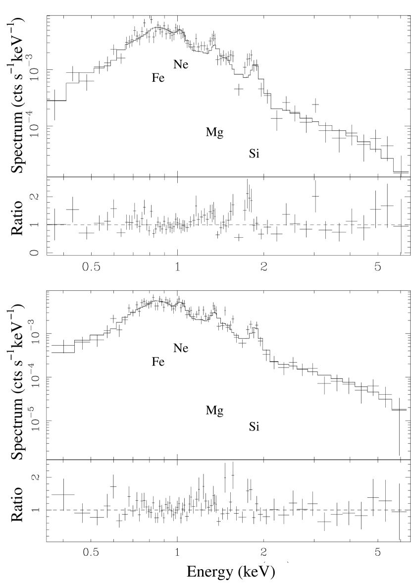
Figure 1: Chandra ACIS-S spectrum of a prominent emission line region of the Antennae hot ISM, before applying the $tgain$ correction (top) and after applying the $tgain$ correction (bottom). The spectrum and the ratio with respect to a thermal+power-law model (XSPEC: wabs(vapec+powerlaw)) are plotted.

We applied corrections to account for the temporal evolution of the ACIS spectral response, caused by changes in the Charge Transfer Inefficiency (CTI) and in the electronic gain of the CCDs. This is a sizeable effect in our case, which we corrected for by applying the time-dependent gain correction described in http://cxc.harvard.edu/contrib/alexey/ tgain/tgain.html. Figure 1 shows a spectrum of a diffuse emission region, plotted before and after the gain correction. A shifting in the emission lines present in the spectrum is evident, with consequences on the quality of the spectral fits (see residual plots in Fig. 1).
The entire data set was then co-added to produce the image of the central part of The Antennae shown in Figure 2.

3 The mapped-color image of the diffuse ISM

Figure 2 shows that complexly structured diffuse X-ray emission is clearly present in The Antennae. Previous work on the 1999 observation alone has shown that this diffuse emission can be related to a hot ISM with varying spatial and spectral properties (Fabbiano et al. 2001; F03). However, our much deeper data show a richness of detail in this diffuse emission that was not visible in the 1999 data alone.

To study this diffuse emission, we followed the procedure of F03 to first subtract the point-like X-ray sources from the data, fill the resulting holes by interpolating the surrounding diffuse emission, and then produce a mapped-color image of the hot ISM. First, from the data we extracted images in three different energy bands: 0.3–0.65 keV, 0.65–1.5 keV and 1.5–6 keV. The middle energy band was chosen to encompass the emission from the Fe-L blend. The 0.3 keV low-energy boundary is the lowest energy within which ACIS is well calibrated. The upper energy boundary was set at 6 keV because at energies $>$6 keV the diffuse emission becomes background-dominated. Then, we used the CIAO tool $wavdetect$ to generate a list of sources detected at a threshold of $3\sigma$ in the co-added exposure, using data in the total 0.3–6 keV energy band within the central 2′ of the image. From this source list, we removed the extended sources listed in Zezas et al. (2002) plus a few additional slightly-extended sources identified by visual inspection of the data. This culling left a total of 127 point-like sources, the positions of which are shown in Figure 2.

We then used the CIAO tool dmfilth to subtract these 127 sources from the data. This tool cuts out the point sources and fills in the holes corresponding to the source positions with values interpolated from the surrounding background regions. We adopted as source regions the $3\sigma$ best fit ellipses computed by $wavdetect$. As background regions we adopted elliptical annuli having the source region ellipse as inner boundary and an ellipse with the same orientation, but with double size semi-minor and semi-major axes, as outer boundary. Areas in the background regions where unrelated sources happened to fall were excluded from the calculation of the background. We used an interpolation technique in which pixel values in the source regions are sampled from the distribution of pixel values in the background regions (dist option in dmfilth), since the Poisson interpolation in the current version of dmfilth does not work for low background regions ($<0.10$ cts/pixel) such as those in the outer parts of The Antennae.

The three diffuse-emission images at different energies were then adaptively smoothed, using csmooth. This process preserves the high-significance small-scale details of the image, while enhancing more extended features of low surface brightness. The same smoothing scales were used for the three images, based on those computed during the smoothing of the 0.65–1.5 keV image, which is the one with the highest signal-to-noise ratio. For the smoothing, we used a Gaussian kernel of varying size (from 1 to 40 pixels). The maximum significance was set to 5$\sigma$, while the maximum smoothing scale corresponds to a minimum significance of $\sim$2.4$\sigma$ for the 0.6–1.5 keV image. The resulting smoothed images were then corrected for exposure (i.e., flat-fielded) by dividing them by the appropriate exposure maps, smoothed using the same scale as the image. The exposure maps were generated for a thermal emission model (Raymond & Smith 1977) with a temperature of 0.8 keV. The resulting exposure-corrected and adaptively-smoothed images, shown in Figure 3, were then combined (using the tool $dmimg2jpg$) to create the “mapped-color” image of the diffuse emission, shown in Figure 4.

In Figure 4, red denotes softer X-ray emission regions (0.3–0.65 keV), while blue denotes harder emission regions (1.5–6 keV). Green identifies emission in the middle band (0.65–1.5 keV). In the following discussion, we will refer to the counts in these bands as $S$ (for soft), $M$ (medium), and $H$ (hard). The color bars in this figure quantify the distribution of the pixel values (from minimum to maximum) in each band.

By comparison with the mapped-color image obtained from the first dataset (ObsID: 0315; F03), the new, deeper image shows an impressive level of detail. Spatial and spectral structures are visible on different spatial scales, from the smaller-scale clumps in the inner parts of the optical merging galaxies to the larger-scale regions of low surface brightness .

Since we have three color-coded energy bands, the resulting pixel color will be ideally distributed in a tridimensional “color cube” whose axis values are proportional to the number of counts in a given band (see right panel of Figure 5). We have “sliced” this cube to obtain a two-dimensional representation that relates the pixel color to the hardness ratios $HR1$ and $HR2$, defined as:

$$HR1=\frac{M-S}{M+S};\>\>\>HR2=\frac{H-M}{H+M}.$$

Each of these slices represents a plane with the same value of hard-band counts (see Figure 5), with soft-band counts increasing along the horizontal axis and medium-band counts increasing vertically. For this chosen value of hard counts, each color in the slice can be uniquely related to a value of $HR1$. These values are written in the bottom slice. The same values will apply to each slice. $HR2$ does not depend on the amount of soft counts, so we display a column of $HR2$ values for each slice, along the “medium-band” axis.

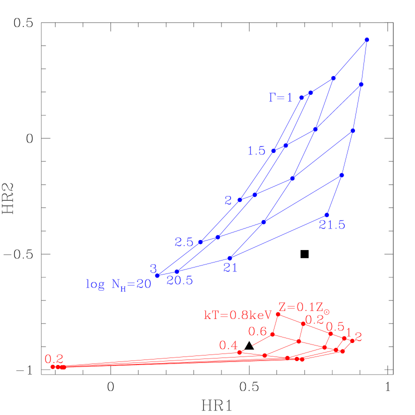
Figure 6: X-ray color-color diagram of $HR1$ vs. $HR2$. The blue grid indicates the regions occupied in the case of a power-law model, varying the intrinsic absorption $N_{H}$ and the photon index $\Gamma$. The red grid represents the loci for a thermal model, varying the temperature $kT$ and the metallicity $Z$. The filled square and triangle indicate the positions in the diagram of the regions described in $\S$3.

It is possible to also give a physical meaning to these numbers, computing the values of $HR1$ and $HR2$ in two cases: an absorbed Raymond & Smith (1977) thermal model and an absorbed power-law model. For the thermal model we vary the temperature from 0.2 keV to 0.8 keV and the metallicity from 0.1 solar to 2 times solar. In the power-law case the photon index $\Gamma$ ranges from 1 to 3 and the intrinsic absorption from $10^{20}$ to $10^{21.5}$ cm^-2. In both cases we considered also a Galactic $N_{H}$ component fixed at the line-of-sight value toward The Antennae ($\sim 3.4\times 10^{20}$ cm^-2; Stark et al. 1992). The values of $HR1$ and $HR2$ are plotted in the X-ray color-color diagram shown in Figure 6, and they can be directly related to the labels in Figure 5. The red grid refers to the thermal model, while the blue grid represents the power-law model. It is likely that a simple single-temperature thermal model or an absorbed power-law model may not be a good fit to the data. However, the figure gives an indication of the characteristics of the X-ray emission from different regions.

For example, the blue region on the bottom-left of Fig. 4 corresponds roughly to $HR1\sim 0.7$ and $HR2\sim-0.5$. Looking at Figure 6, these hardness ratios—marked by a black square—are located at a point in the diagram between the absorbed-power-law model and the purely thermal model, possibly indicating the presence of unresolved binary emission in this region. On the other hand the orange region on the right of Fig. 4 corresponds roughly to $HR1\sim 0.5$ and $HR2\sim-0.9$ (black triangle in Figure 6). These values are typical of purely thermal emission.

4 The Line-Strength Map

As Figure 1 illustrates, the spectra extracted from different regions of the diffuse emission frequently show emission lines. In particular, O+Fe+Ne emission (0.6–1.16 keV) is often present, together with Mg-XI (1.27–1.38 keV) and Si-XIII (1.75–1.95 keV) lines. Using these features, we generated another color map (see Fabbiano et al. 2004) that gives a qualitative representation of the presence of emission lines from Iron, Silicon, and Magnesium in different regions of the hot ISM. This map has proven very useful for identifying regions of strong apparent line emission and for selecting spectrally similar regions for a proper spectral analysis.

The line-strength map, shown in Fig. 7a, was constructed as follows. First, we created images in three bands encompassing emission from O+Fe+Ne (0.6–1.16 keV), the Mg-XI line (1.27–1.38 keV), and the Si-XIII line (1.75–1.95 keV). We also created an image including emission in the 1.4–1.65 keV and 2.05–3.05 keV bands, which was used for continuum subtraction. The line and the continuum bands were determined from spectra of the diffuse emission in order to have an optimum line/continuum ratio and minimal contamination by emission lines, respectively. In each band we excluded all point-like sources and interpolated over the holes as described in § 3. The O+Fe+Ne band image, which contains a much larger number of counts than the other line-band images, was used to determine the smoothing scales, and was adaptively smoothed to a significance between 3$\sigma$ and 5$\sigma$. The same smoothing scales were then also applied to the other line and continuum images. In order to subtract the appropriate continuum from each line image, the continuum image was rescaled to represent the band continuum in the given line. To calculate the weighting factors, we extracted the spectrum of the entire diffuse emission of The Antennae and fitted the continuum (after excluding the energy ranges with line emission) with a two-component Bremsstrahlung model. Based on this model we estimated the relative intensity of the continuum in our continuum band and the three line bands. Each line image was continuum subtracted after weighting the continuum image by these weighting factors, and the resulting images were combined to create a mapped-color line-strength image (Figure 7a). In this image, red represents line emission from O+Fe+Ne, green from Magnesium, and blue from Silicon, respectively.

Figure 7a shows that the hot ISM of The Antennae has a complex emission-line structure. Silicon emission (blue) appears pervasive in most of the hot ISM, with Magnesium lines (green) also present in various relative amounts and O+Fe+Ne emission (red) prevalent in some regions. Other regions (black) show only very weak or no line emission.

5 Spectral Analysis

The mapped-color X-ray image (Figure 4) and the line-strength map (Figure 7a) demonstrate that the diffuse emission of the hot ISM is rich in spatial and spectral features, and that the line emission in the X-ray spectra is pervasive and varied. These figures suggest a temperature structure in the hot ISM, possibly the effect of varying absorption on the emission (see also F03), and of its metal enrichment.

5.1 Region Selection and Extraction of the X-ray Spectra

To put these results on a more rigorous and quantitative footing, we have performed a spectral analysis of different regions of the hot ISM, using Figures 4 and 7a as guides for the selection of these regions. We first identified 17 separate regions for analysis, based on the morphology of the diffuse X-ray emission (Fig. 7a). However, the line-strength map suggested marked abundance differences within some of these regions. In particular, Figure 7a shows that regions 4, 6, 8, and 12 have a complex metallicity structure. For example, in Region 4 we can identify a metal-rich and a metal-poor area; in regions 6, 8, and 12 we see clearly defined sub-areas with yellow (O+Fe+Ne and Mg) and red (O+Fe+Ne) emission. These four regions also have a very high number of detected counts, making it possible for us to subdivide them further on the basis of their line features. We subdivided each of these four regions into two parts, as shown in Figure 7b. Although Figure 7a suggests spatially complex metal distributions also in other regions (5, 13, 14 and 15), these regions have too few counts to be subdivided further. The described process identified a total of 21 regions for separate spectral analysis.

From these 21 regions, we excluded all the point source $3\sigma$ areas described in § 3 and shown in Figure 2. We then extracted background counts representative of the field from three circular source-free regions well outside the galaxies, but within the same CCD (ACIS-S3) in all seven observations. These background regions covered a total area of $\sim$4 arcmin².

All of the data sets under analysis, with the exclusion of the first and fifth (ObsID: 315 and 3044, respectively), were obtained with the same ACIS-S configuration and could then be treated as a single observation. We therefore merged these data into a single event file by using the CIAO script $merge$_$all$. ObsID 315 and 3044, however, needed individual handling. ObsID 315 was obtained in 1999 December, when the low-energy response of ACIS-S was significantly higher ($A_{eff}\sim 500$ cm², $QE\sim 65\%$ at 1 keV) than at the time of the other six observations (2001 December to 2002 November). ObsID 3044 was obtained with a different ACIS-S configuration (different SIM-Z).

We extracted spectra separately from the merged 5-ObsID file and from 315 and 3044, using the diffuse emission and background areas described above. In all cases, the CIAO script $acisspec$ was used to extract the region spectra. This script invokes the tool $dmextract$ to extract the spectrum and then uses the tools $mkwrmf$ and $mkwarf$ to create area-weighted Response Matrix Files (RMF) and Ancillary Response Files (ARF) for each region, since they span more than one FITS Embedded Function (FEF) region. The spectra derived from the three different event files, both from source and background regions, were then summed using the FTOOL $mathpha$. The response files were combined with their appropriate weights, using the FTOOLS $addrmf$ and $addarf$. The resulting spectra were then grouped so as to have at least 20 counts per energy bin before background subtraction.

For each of the 21 regions used in the spectral analysis the net counts (background subtracted) in three different energy bands and in the total 0.3-6.0 keV band are listed in Table 2.

5.2 Spectral Fit Method

We analyzed the extracted spectra with XSPEC v11.2.0 (Arnaud 1996), using combinations of optically-thin thermal emission and power-law components to fit the data. We used the Astrophysical Plasma Emission Code (APEC) thermal-emission model (Smith et al. 2001) to represent the thermal emission. This model is based on the original Raymond & Smith (1977) code, but has been totally revamped to exploit modern computing capabilities and the wealth of accurate atomic data.

The real nature of a soft X-ray emitting gas, recently heated as in star-forming galaxies, is clearly that of a multi-temperature plasma with very complex differential emission-measure distributions (see, e.g., Strickland & Stevens 2000). Since the gas is continuously being heated by SN and star winds, it may also not be in ionization equilibrium. However, modeling our low S/N spectra with complex models having more than two temperatures or not assuming ionization equilibrium would require too many free parameters to obtain any meaningful information from them. For example, although fitting higher S/N spectra of diffuse X-ray emission in nearby starburst galaxies with two-temperature models (using combinations of several equilibrium and non-equilibrium models) frequently leads to better fits than fitting with a single-temperature model (e.g., NGC 253: Strickland et al. 2002), they almost always lead to unrealistically low abundances, as previously noted by Metz et al.(2004). Therefore, we considered also single-temperature models to fit our data, together with two-temperature models, to allow us to compare the results obtained from both. The four models that we used, listed in order of increasing complexity, are:

• absorbed one-temperature APEC model (XSPEC model: wabs(wabs(vapec)));

• absorbed one-temperature APEC model plus a power-law component (XSPEC model: wabs(wabs(vapec+pow)));

• absorbed two-temperature APEC model (XSPEC model: wabs(wabs(vapec+vapec))); and

• absorbed two-temperature APEC model plus a power-law component (XSPEC model: wabs(wabs(vapec+vapec+pow))).

Two different absorption components were used in all cases: one fixed at the Galactic line-of-sight value toward The Antennae ($N_{H}=3.4\times 10^{20}$ cm^-2; Stark et al. 1992) and the other one left free to vary in order to model the intrinsic absorption within the two galaxies. In the two models where a power-law component is included we tried also to fit the $N_{H}$ absorption independently for the power-law and thermal components. Although the $N_{H}$ of the power-law component resulted in a value different from the $N_{H}$ of the thermal component(s) (on average $\sim 10^{21}$ cm^-2 instead of $\sim 10^{20}$ cm^-2), the best fit parameters of the thermal component (mainly $kT$ and $Z$) did not vary significantly and were fully consistent within the errors. The abundances of Neon, Magnesium, Silicon, and Iron were all left free to vary. The other elements (e.g., Carbon, Nitrogen, and Sulfur) are poorly constrained because of gain uncertainties and sensitivity to $N_{H}$. Thus we adopted solar abundances for these elements. We tried to thaw the Oxygen abundance, obtaining no clear improvements in the fits and no significant variations in the best-fit parameters of $kT$ and of $Z$ in the other elements. Moreover, the poorly costrained Oxygen abundance values were always consistent with solar values. Therefore, we decided to adopt a solar abundance also for this element.

We introduced a power-law component into our models to allow for the possible residual presence of unresolved X-ray binaries too faint to be detected individually. Indeed, from an analysis of the entire emission throughout The Antennae we found that the point sources contribute up to $\sim$85% of the emission in the 2–5 keV range and are essentially the only contributors above 5 keV. The photon index value was at first frozen at $\Gamma=1.88$, a value obtained by fitting the 2–10 keV spectrum of the entire emission from The Antennae, including point sources. Afterwards $\Gamma$ was left free to vary to fit the data in order to test for the presence of substantial discrepancies between the average power law determined from the galaxies’ global emission and possible power-law components in individual regions. We compared the results of the two fits (frozen and thawed $\Gamma$) for the same region using an F-test, and considered the thawed $\Gamma$ model to be a better description of the data if $p$, the probability that the improvement in the $\chi^{2}$ statistics is due by chance, was less than 5%.

The resulting best-fit temperature(s) $kT$, absorbing column density $N_{H}$, and power-law photon index $\Gamma$ (if a power-law component is necessary) for the 21 regions studied are summarized in Table LABEL:mytable1old, together with the abundances of Neon, Magnesium, Silicon, and Iron relative to the solar values. The last column of Table LABEL:mytable1 gives the “best-fit model”. The errors are quoted at $1\sigma$ for one interesting parameters. The values listed in the table are obtained from the “best-fit model”, which is defined as the simpler model (i.e. with a smaller number of parameters to be fitted) with $\chi^{2}_{red}<1.4$. This value of $\chi^{2}_{red}$ represents a fair boundary between an acceptable fit and a bad fit for low S/N spectra (0.3–6 keV counts in the range between $\sim 750$ and $\sim 6500$). This means that we do not adopt a two-temperature model if an acceptable fit is already obtained with only one temperature. We understand that a single-temperature and even a two-temperature model are approximations to the real physical nature of the X-ray emitting gas, which is likely to be more complex. However, given the limitations of our data we followed the customary data analysis practice of choosing the simpler model of two if both models give acceptable representations of the data. Indeed, we found that only one region does not yield an acceptable fit using a single-temperature spectral model (Region 4b). Possible systematic biases depending on the model choice are taken into account as explained in § 5.2.1 below. The only region where none of our models yielded a $\chi^{2}_{red}<1.4$ (although with only 751 counts in the 0.3–6 keV band) is Region 13, for which we chose the model with the lowest $\chi^{2}_{red}$. The spectra of the 21 regions, together with the best-fit models and the data-to-best-fit-model ratios, are shown in Figures 8, 9, 10, and 11.

5.2.1 Error computation

Although quoting the errors at $1\sigma$ for one interesting parameter (as the errors quoted in Table LABEL:mytable1old) is a common practice in X-ray spectral analysis, it may lead to an underestimation of the true uncertainties not only because of possible systematics but also in the case that some of the fitting parameters are correlated. As previously noted by Martin, Kobulnicky & Heckman (2002) a degeneracy between metallicity and temperature may exist in the spectral models, and it is very difficult to solve such ambiguity from low resolution CCD spectra like the ones we are dealing with. Indeed we found such a degeneracy at least in some of our regions. Although it will not be possible to solve completely this problem from the spectral analysis of ACIS spectra alone, it is still possible to adopt a very conservative approach to take into account both systematics and correlations between fitting parameters. This approach mainly consists in calculating the errors for the best-fit parameters at 1$\sigma$ for all interesting parameters. The errors on $kT$, $N_{H}$, and $\Gamma$ were calculated from the $\chi^{2}$ statistics considering all free parameters in the “best-fit model” as interesting. Since the spectral regions occupied by Ne, Mg, and Si lines are quite distinct, the errors on the abundances for these elements were computed using a different method to reduce the number of interesting parameters. We first attempted to link together all the $\alpha$ elements using the type II SNe ratio from the compilation of average stellar yields from Nagataki & Sato (1998), in order to reduce the number of free parameters by two. However, we were unable to obtain acceptable fits for any of the regions, suggesting that the elemental ratios are not entirely consistent with type II SN yield models. Thus we tried an alternative approach for each individual $\alpha$-element line, ignoring from the fit the part of the spectrum relative to the other two lines (e.g. for Mg we ignored the part of the spectrum occupied by the lines of Ne and Si) and freezing their abundances to their best-fit values. Therefore, in the error computation of the $\alpha$-elements we have two free parameters less than in the computation of $kT$, $N_{H}$, and $\Gamma$. For deriving the Fe abundance we ignored the part of the spectrum relative to all three $\alpha$ elements (freezing them to their best-fit values), obtaining three less free parameters than the original model. The number of interesting parameters was set equal to the number of free parameters also for the abundance error estimation. Note that this is a very conservative approach for the determination of statistical errors, since the fitting parameters are not completely independent from each other, so that the number of truly interesting parameters is likely to be lower than the one adopted. However, statistical errors are not the only uncertainties present in our measurements, and systematic biases may arise also from the spectral model choice, as noted before in § 5.2. Although our method cannot estimate exactly any possible systematics, it is conservative enough that we are confident about the parameter confidence ranges so derived. The best-fit parameters and the errors computed using this method are shown in Table LABEL:mytable1. Comparing this table with Table LABEL:mytable1old, it is clear that the abundances measured using the method described above are consistent with the measures performed fitting the whole spectrum. The only noticeable difference comes from the 1$\sigma$ confidence ranges which, of course, are larger in Table LABEL:mytable1. In the rest of the paper we will use the confidence ranges of Table LABEL:mytable1.

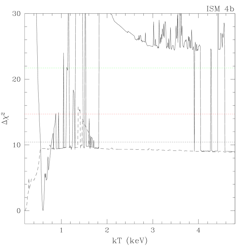
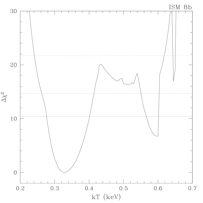
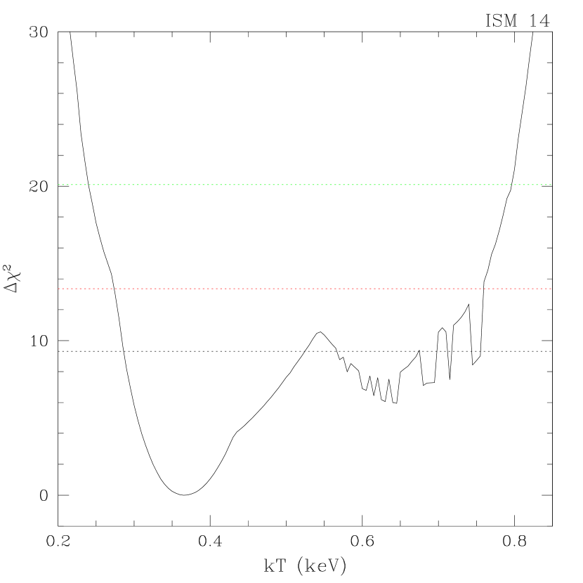
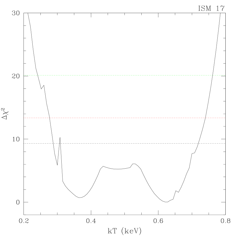
Figure 12: Distribution of the $\Delta\chi^{2}$ values as a function of the temperature in four of our regions chosen for spectral analysis. The black dashed line in the upper-left panel represents the $\Delta\chi^{2}$ distribution as a function of the lower temperature in a two-temperature best-fit model. The black dotted line, the red dotted line, and the green dotted line represent the 68%, 90% and 99% confidence levels, respectively.

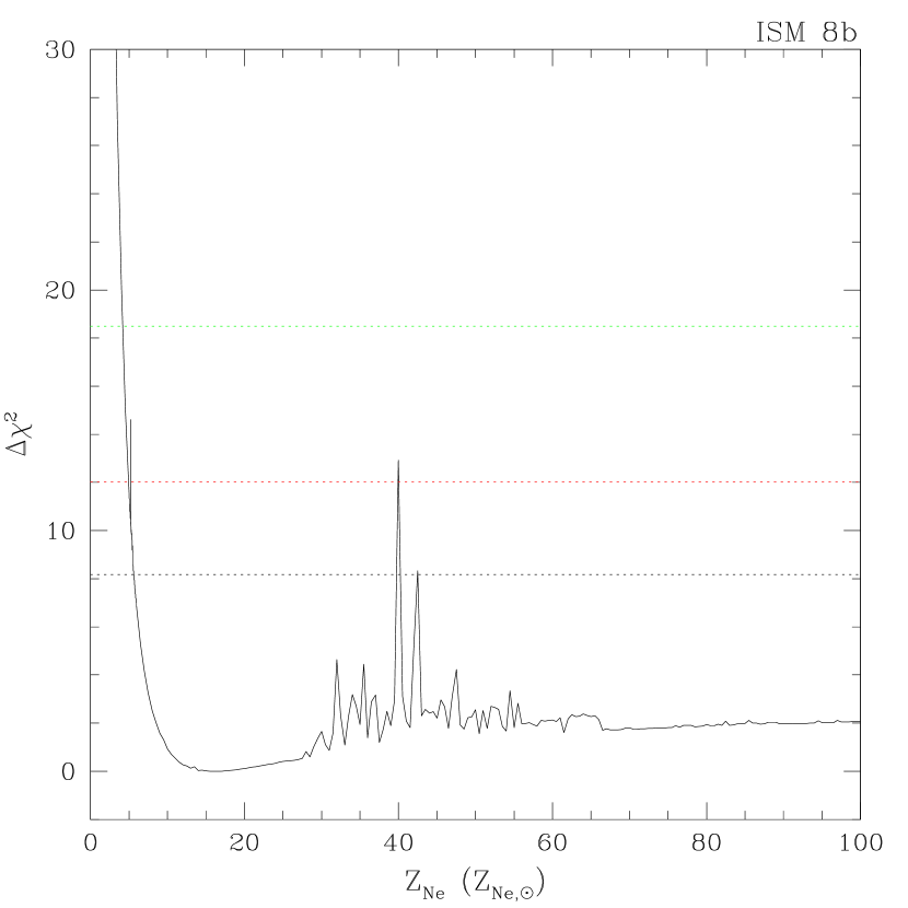
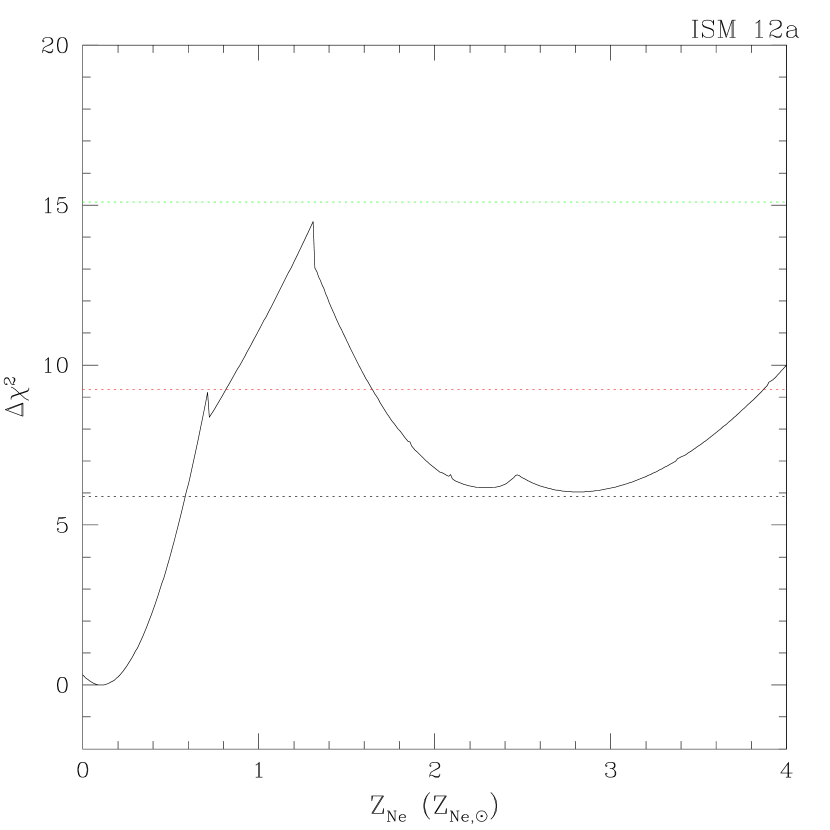
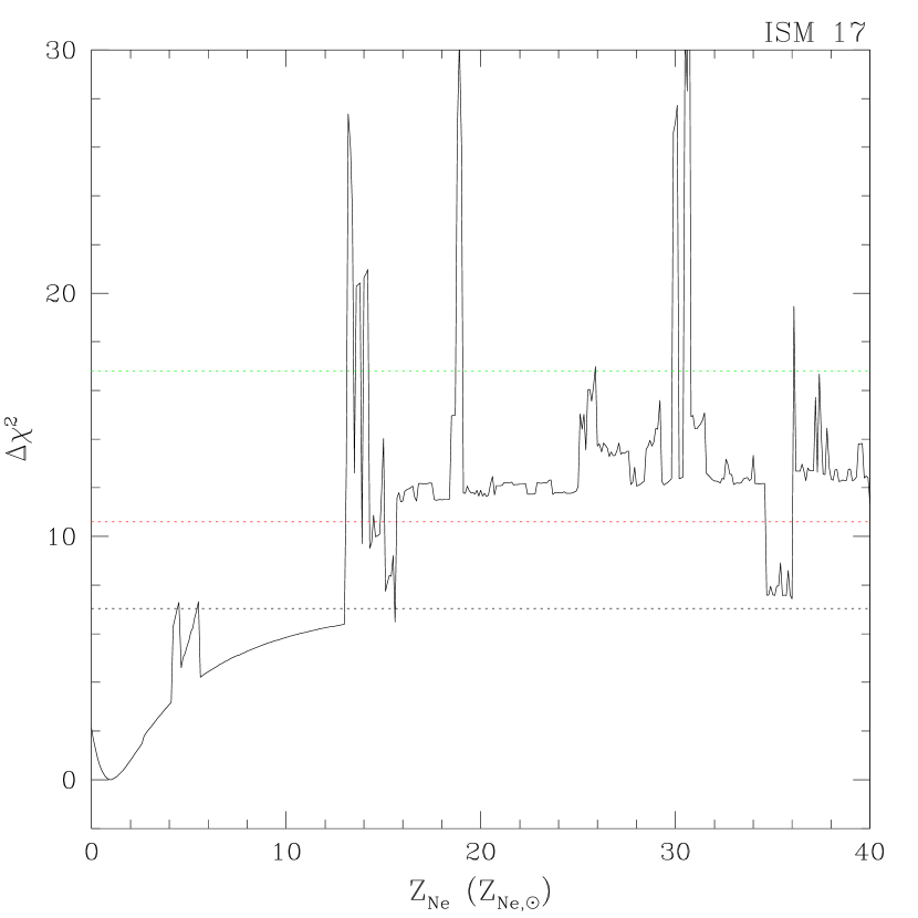
Figure 13: Distribution of the $\Delta\chi^{2}$ values as a function of the Neon abundance in four of our regions chosen for spectral analysis. The black dotted line, the red dotted line, and the green dotted line represents the 68%, 90% and 99% confidence levels, respectively.

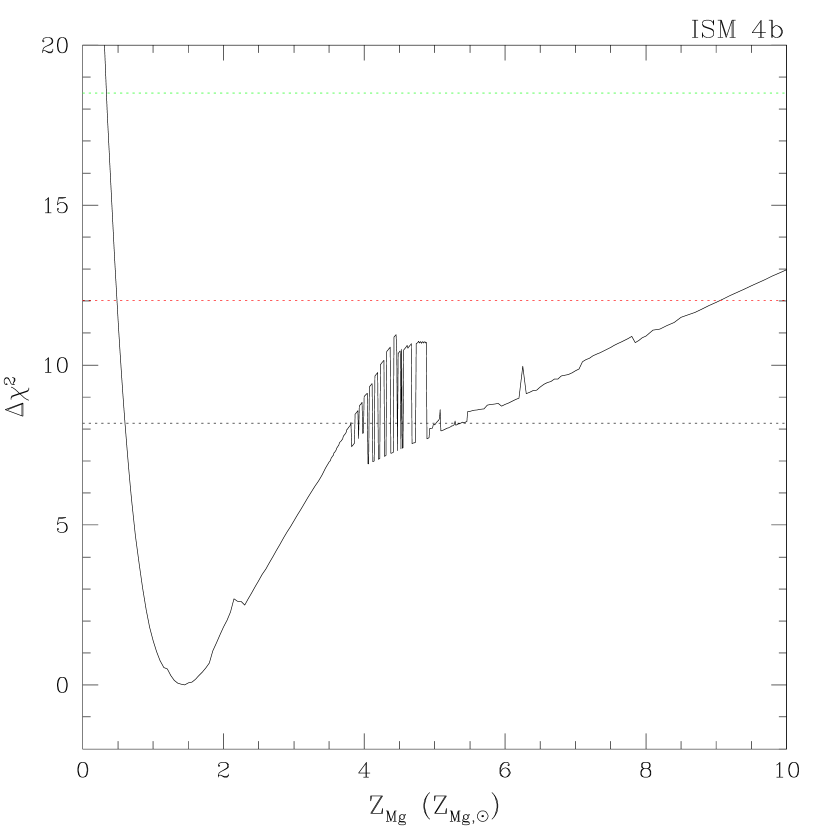
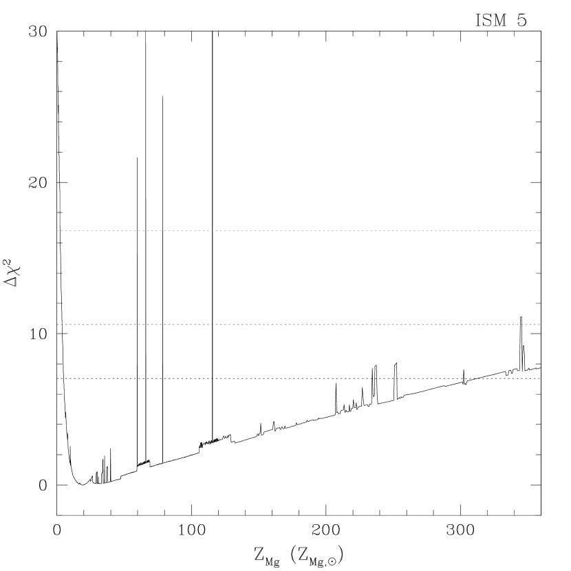
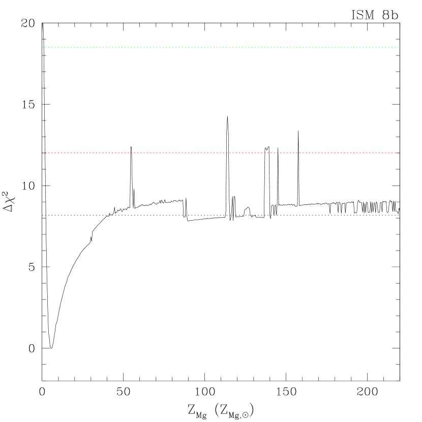
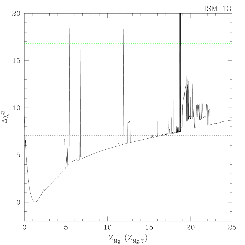
Figure 14: Distribution of the $\Delta\chi^{2}$ values as a function of the Magnesium abundance in four of our regions chosen for spectral analysis. The black dotted line, the red dotted line, and the green dotted line represent the 68%, 90% and 99% confidence levels, respectively.

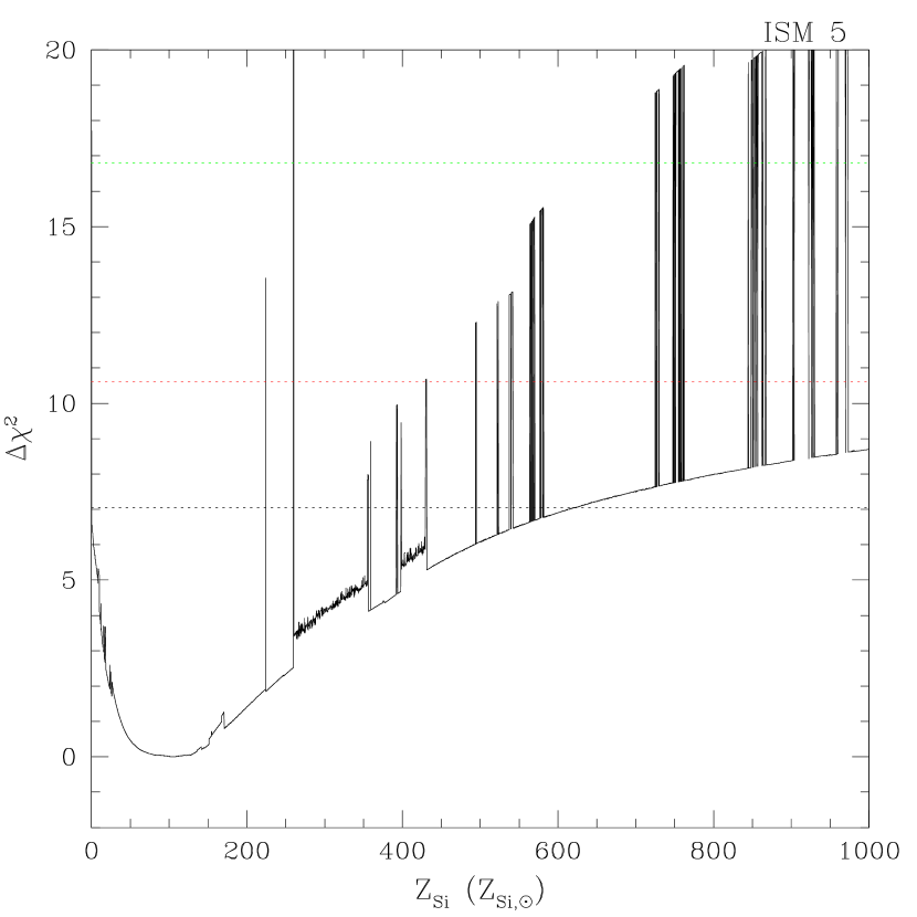
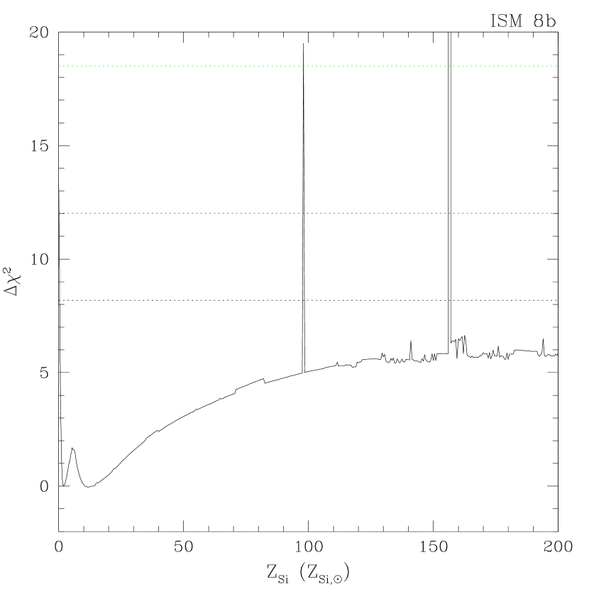
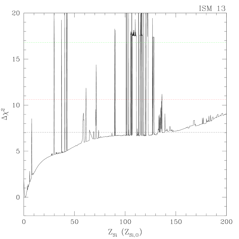
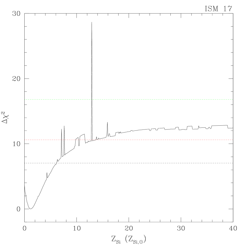
Figure 15: Distribution of the $\Delta\chi^{2}$ values as a function of the Silicon abundance in four of our regions chosen for spectral analysis. The black dotted line, the red dotted line, and the green dotted line represent the 68%, 90% and 99% confidence levels, respectively.

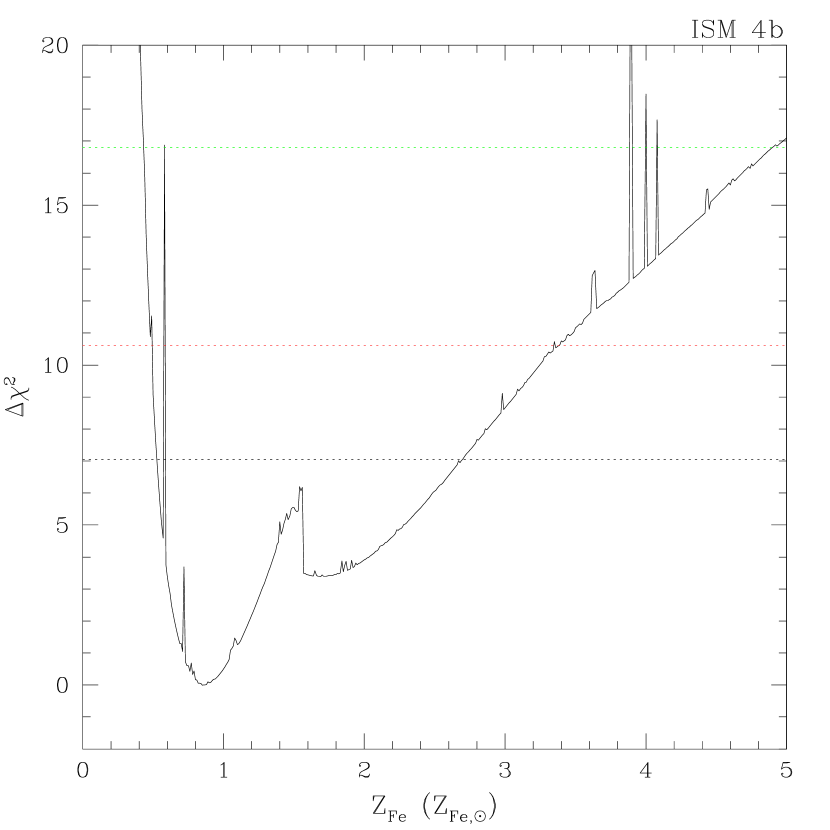
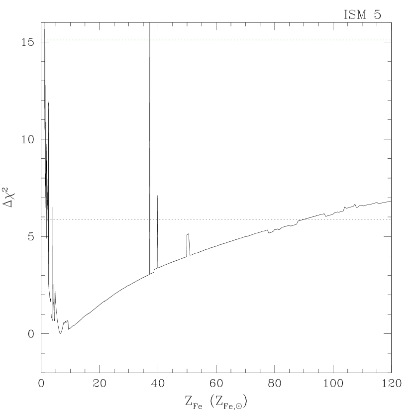
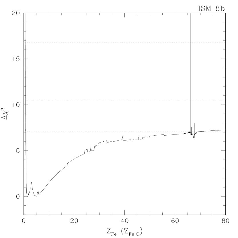
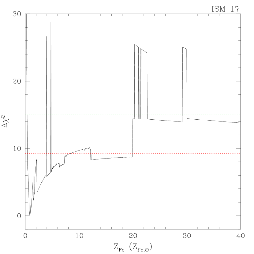
Figure 16: Distribution of the $\Delta\chi^{2}$ values as a function of the Iron abundance in four of our regions chosen for spectral analysis. The black dotted line, the red dotted line, and the green dotted line represent the 68%, 90% and 99% confidence levels, respectively.

The $\chi^{2}$ parameter space is often asymmetric. Therefore, we performed an analysis of the behaviour of $\chi^{2}$ with each free parameter (using the steppar command in XSPEC), to explore the presence of possible secondary $\chi^{2}$ minima in the confidence range estimation. Figures 12–16 show some examples of the most complicated features observed in the $\chi^{2}$ parameter space when varying the temperature ($kT$) and the abundances of Ne, Mg, Si and Fe, respectively. As can be seen in Figure 12, one of the temperatures of Region 4b is unconstrained even at the $1\sigma$ level. Three other regions (8b, 14 and 17) show two minima in $\chi^{2}$ space. For them we adopted $1\sigma$ confidence ranges encompassing both minima even when the $\Delta\chi^{2}$ value between them exceeded the $1\sigma$ confidence level, as happens in Regions 8b and 14. For abundances the presence of secondary minima is more rare: we found a secondary minimum only in Region 8b (Si and Fe; Figs. 15 and 16) and in Region 4b (Fe; Fig. 16).

5.2.2 Emission-line equivalent width

While spectral fits are the standard way to obtain elemental abundances from X-ray data, we also wish to obtain abundance limits that are relatively model-independent and that allow us to evaluate the possible effects of departures from ionization equilibrium (NEI). Since in our spectra the lines of Mg and Si are not confused with other elements, they allow us to directly measure their equivalent widths (hereafter $EW$). For each region we considered the spectrum in the whole 0.3–6 keV range and used the best-fit model (as defined in § 5.2) for the continuum. We artificially set to zero the abundance of the element in consideration, adding a gaussian line to the model. Both the normalization and the energy of the gaussian line were left free to vary in the fit. From the best fit so obtained we measured the $EW$ of the line using the XSPEC task eqwidth, using only the thermal component(s) as continuum emission. With eqwidth we performed a Monte Carlo sampling of the parameter values distribution, estimating the errors on the $EW$ (at $1\sigma$) independently from the $\chi^{2}$ statistics. The relation between the measured $EW$ and the measured abundance for Mg and Si are shown in Figure 17. We find a clear correlation between the two parameters for Mg; a weaker correlation is suggested by the Si plot, however we must remember that the continuum is much less well defined for this line, increasing the uncertainties.

The metal abundances measured from the spectral fits can be directly related to the $EW$s by the expression:

$$EW=\frac{a\cdot Z}{1+\alpha\cdot Z},$$

where $Z$ is the abundance of the element and $a$ and $\alpha$ are two parameters essentially dependent only on the temperature of a hot X-ray emitting gas in a static ionization equilibrium. The denominator comes about because the continuum is produced by bremsstrahlung and the recombination of lower atomic number elements, while the numerator is simply proportional to the abundance of the element in question. The temperature dependence arises mostly from the ionization fractions of the H-like and He-like ions that produce the emission lines. The term $\alpha$Z in the denominator accounts for the contributions of all the elements other than H and He to the continuum through bremsstrahlung, recombination, and two-photon emission assuming that all the elements scale together. Thus at very high Z the EW will reach an asymptotic limit, which can only be exceeded if the element in question is preferentially enhanced relative to the elements that contribute to the nearby continuum or if NEI increases the equivalent width. In order to assess the likely effects of NEI we computed equivalent widths from shock wave models using an updated version of the code described in Raymond (1979) and Cox and Raymond (1985). While the EW can be far from the equilibrium values just behind the shock, it tends to be dominated by emission from the region that is not too far from equilibrium. We computed models for shocks in the range 400–900 km/s, corresponding to a temperature immediately behind the shock between 0.19 and 0.95 keV. Note that in the latter case the temperature that would be derived from the X-ray continuum would be somewhat lower because of contributions from gas in the cooling region.

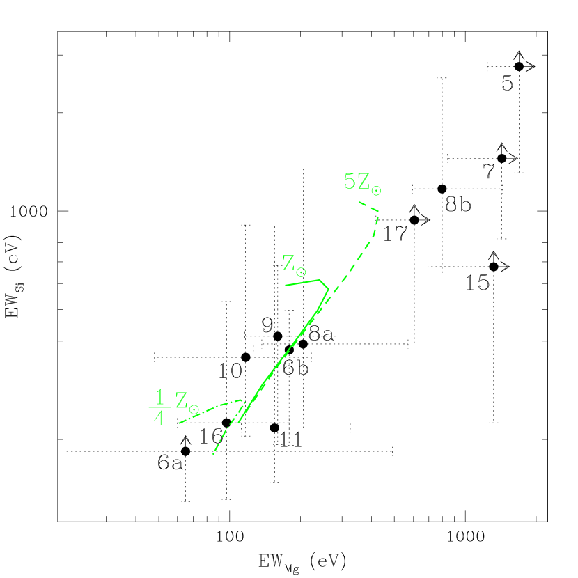
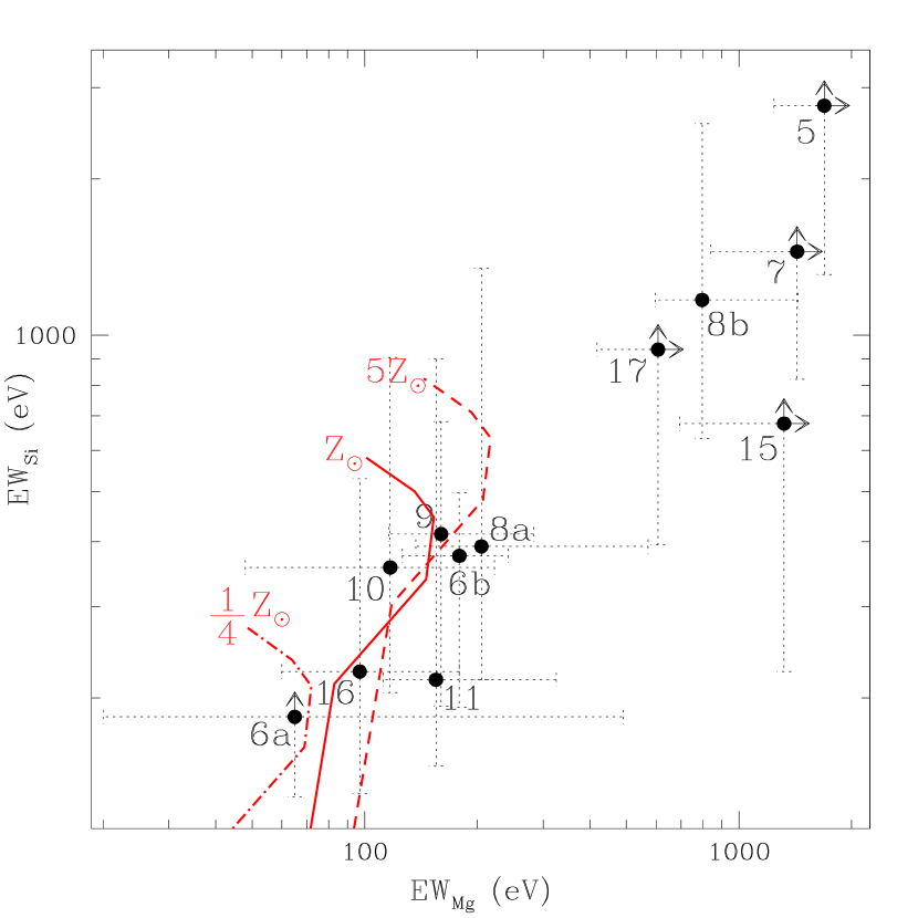
Figure 18: Measured $EW$ of the Mg line vs. measured $EW$ of the Si line for the hot ISM regions of the spectral analysis. Right: the green lines represent the expected $EW$s as a function of the temperature (growing with growing values of $EW_{Si}$; for details, see text) for a plasma in ionization equilibrium with $Z=\frac{1}{4}Z_{\odot}$, $Z=Z_{\odot}$ and $Z=5Z_{\odot}$. Right: the red lines represent the expected $EW$s as a function of the shock velocity (growing with growing values of $EW_{Si}$; for details, see text) for a shock-heated plasma with $Z=\frac{1}{4}Z_{\odot}$, $Z=Z_{\odot}$ and $Z=5Z_{\odot}$

Using the values of $\alpha$ and $a$ computed for the two different cases examined (thermal plasma and shock waves) we derived the expected $EW$ corresponding to an abundance of $\frac{1}{4}Z_{\odot}$, $Z_{\odot}$ and $5Z_{\odot}$ for both Mg and Si. Figure 18 shows the relation between the $EW$ of Mg and the $EW$ of Si for all the regions where we were able to obtain a meaningful measure of both. The regions of the diagram relative to abundances of $\frac{1}{4}Z_{\odot}$, $Z_{\odot}$ and $5Z_{\odot}$, as a function of the temperature are also plotted. If we consider the simple equilibrium thermal model (Fig. 18, left) the majority of the points are located in the region corresponding to solar abundance, but there are regions located in the upper-right portion of the diagram as well. Region 5 has $EW$ not consistent with $Z\leq 5Z_{\odot}$ for both elements, in agreement with the results of the spectral analysis where this region shows the highest abundances of Mg and Si among all the spectra analyzed. Also Regions 7, 8b, 15, and 17 show high values of the $EW$, but with large errors, consistently with what we observe in the abundances measured from the spectral analysis of these regions. The situation is even more dramatic if we consider the shock model (Fig. 18, right), where the values of Mg for the regions listed above are clearly not consistent with $Z<5Z_{\odot}$ (as the spectral analysis would suggest), and the Silicon $EW$ for Region 7 is also not consistent with $Z<5Z_{\odot}$. Notice that the values of the $EW$ we derived from the abundances at the different temperatures were computed assuming that all the elements scale together at the same time. Thus the continuum due to lower $Z$ elements contributes at the energies of the emission lines. If Mg or Si are enhanced relative to O in particular, the equivalent width expected could be higher. That would require that the enrichment in The Antennae is done by supernovae with a different mass distribution than those that enriched the solar neighborhood (e.g. Woosley & Weaver 1995). This is indeed likely for very young star forming regions, in which only the most massive stars will have completed their evolution. We note that departures from ionization equilibrium other than those of the shock models are possible if the plasma is rapidly heated or cooled. In general they do not raise the EW very much above the equilibrium values except in a very strongly overionized, cool plasma (e.g. Breitschwerdt & Schmutzler 1994). While it is possible to produce such a plasma by rapid adiabatic expansion, the low emissivity makes it difficult for such a plasma to make a significant contribution to the spectrum.

5.3 Comparison with results from the first Chandra observation

Almost all the regions (20 out of 21) did not require the presence of a second thermal component in the model to fit the data, and half of them (11 out of 21) did not need the presence of a power-law component to fit the data. In the cases where the power-law component was needed, the fixed $\Gamma=1.88$ models were found to yield a better fit than a thawed $\Gamma$ model in eight regions out of 10. Only Region 4b required two thermal components with different $kT$. In this region, we could not constrain the low $kT$ value (although we found a minimum in the $\chi^{2}$ statistics at $kT=0.20$) and we could place only a lower limit ($kT>0.54$) on the higher temperature component. Almost all the single-temperature regions required a temperature of $kT\sim 0.6$ keV to fit the data, with regions 5, 8b, and 14 ($kT\sim 0.3$ keV) the only exceptions to this rule. Considering all the regions analyzed, the temperatures (both in the single- and double-temperature cases) range from $\sim 0.2$ to $\sim 0.8$ keV (considering also the errors), a range fully consistent with the values found in F03.

F03, however, could not reach any conclusions about the metal abundances of the ISM because of the shorter integration time of their data set (only ObsID 315). In contrast, our analysis yields metal abundances that have acceptable constraints in the majority of the regions. This represents the most striking new result of our spectral analysis: the abundances of Silicon and Magnesium cover a wide range of values from the very low values found in regions like Region 2, 6a, 12a, and 12b ($Z\sim 0.2Z_{\odot}$) to the huge values observed in Region 5 ($Z\geq 20Z_{\odot}$).

The intrinsic absorption throughout the hot ISM is generally low, with typical $N_{H}\sim 10^{20}$ cm^-2 and often consistent with zero. The exceptions are the southern nucleus (regions 8a and 8b) and Region 7 (the dark-blue area in Figure 4), which is significantly obscured also in the optical. Region 7 corresponds to the Overlap Region, where the most active star formation is now occurring (Mirabel et al. 1998; Wilson et al. 2000; Zhang et al. 2001). These regions show intrinsic absorption corresponding to $N_{H}\sim 1-2\times 10^{21}$ cm^-2.

A direct comparison with the results of the spectral analysis performed on ObsID 315 in F03 can be done for the four emission regions identified and analyzed individually in that paper: the northern nucleus (roughly corresponding to our regions 14 and 15), the southern nucleus (regions 8a, 8b, and 9), the hot spot R1 (regions 12a and 12b), and the hot spot R2 (Region 13).

In the northern nucleus F03 found $kT\sim 0.6$ keV, which is fully consistent with the temperatures we found in regions 14 and 15 ($0.37_{-0.08}^{+0.39}$ and $0.59_{-0.14}^{+0.09}$ keV, respectively). The best-fit abundances given in F03 ($\sim$0.15 solar) are lower than our solar or slightly sub-solar abundances observed in Region 15 (in Region 14 abundances are unconstrained); however, the large errors encompass our results.

The southern nucleus in F03 is well fitted by a two-temperature model, with temperatures (0.35 and 0.82 keV) consistent within the errors with the two peaks in $\chi^{2}$-space observed for the temperatures of our Region 8b (0.33 and 0.60 keV). However, in regions 8a and 9 we find a single temperature gas at $\sim$0.6 keV. Also in this case the abundances in F03 are very low ($\sim$0.2 solar), in contrast to abundances consistent with solar in all the three regions we examined. In this case as well, though, the abundances determined by F03 are poorly constrained and consistent with our results.

In F03 the hot-spot R1 was fitted with a single-temperature model at $\sim$0.4 keV, while the temperatures we find are somewhat higher, with $0.60_{-0.09}^{+0.05}$ keV and $0.61\pm 0.06$ keV for regions 12a and 12b, respectively. F03 determined a value of $\sim$0.2 solar for the abundance, which is fully consistent with the low values we find in both Region 12a and Region 12b.

For the hot spot R2 the only comparison possible is for the temperature (F03 could not constrain the abundance), which was $\sim$0.4 keV in F03, somewhat lower than the value in Region 13 ($kT=0.58_{-0.35}^{+0.09}$ keV). However, the large errors in our new temperature determination (due to a secondary minimum in the $\chi^{2}$, as described in § 5.2.1) make these two results consistent.

The lower metal-abundance values suggested by the F03 analysis could be the result of blending of complex emission regions. Note, however, that in F03 all elements were kept locked at the solar ratio, while we have here fitted the abundances of Fe, Mg, Ne, and Si individually.

Some of the 21 regions we have chosen are similar to, though not quite the same as, several of those analyzed by Metz et al. (2004). Our regions 2, 4, 5, 6, 12, 13 14 and 15 roughly correspond to their regions D03, D06, D07, D08, D01, D02, D04 and D05, respectively. In general, our and their spectral results are similar, except that the higher quality of our spectra permits at least a coarse measurement of elemental abundances in contrast with their assumption of solar abundances throughout the hot ISM.

5.4 Comparison with ASCA Results

The high metal abundances suggested by our spectral analysis in some regions of The Antennae are at odds with a previous claim, based on ASCA CCD spectra, of an overall extremely low abundance of heavy elements in this system ($\sim$0.1 the solar value, Sansom et al. 1996). Since the spectral resolution of ASCA was comparable to that of Chandra ACIS, we explore the possibility that—besides the lower signal-to-noise ratio of the previous data—poor spatial resolution may have played a role in the low abundances reported from the analysis of the ASCA observations.

Given the large ($\sim 2$ arcmin) ASCA beam, the entire emission from The Antennae was used to derive a spectrum. To make a fair comparison with the ASCA data, we extracted from our Chandra data a spectrum of all 21 regions together, leaving the point sources (which could not be excluded in the ASCA observation) in the extraction region. We used the procedure described in § 5.1 to extract the spectra and compute response matrices individually for the first (December 1999) and the fifth (July 2001) observation, and from a merged event file for the other five observations combined. The background was taken from the same areas used in the case of the individual regions’ analysis. The combined spectra and response matrices were used in XSPEC. The spectrum was fitted using a model with two additive components: a Raymond-Smith thermal model (for the diffuse emission) and a power law (for the point sources). To repeat the ASCA analysis we assumed a solar abundance ratio between the various elements, and fitted the metal abundance with just one parameter. We considered two different components for the absorption, one fixed at the Galactic value and the other left free to vary to measure the intrinsic absorption within The Antennae. The quality of the fit we obtained is very poor ($\chi^{2}_{\nu}\sim 2.8$), not surprisingly given the complexity of the temperature and metallicity distributions throughout The Antennae. However, the best-fit model has a temperature of $kT=0.59\pm 0.03$ keV and a metallicity of $0.18_{-0.08}^{+0.15}$ times the solar value, fully consistent with the ASCA results (Sansom et al. 1996). This demonstrates that the analysis of separate “clean” regions, possible because of the sub-arcsecond resolution of Chandra, is needed to detect the metal lines in a complex hot ISM with CCD spectral resolution.

The above conclusion is reinforced by the intercomparison of the spectral-fit results for different subsections of morphologically selected regions (e.g., regions 5 and 12b), where the line-strength map of Figure 7a suggested different metal contents in the spectra. The results of these fits are compiled in Table 3 and clearly present intermediate metal abundances, typically lower than the peak value. We note that while the spatial resolution of Chandra surpasses that of any other X-ray telescope it is still finite, and while our exposure of The Antennae is deep the collecting area of Chandra is limited. Therefore, our results on metal abundances by necessity still suffer to some degree from an “averaging” effect over spectrally complex regions. As such, they may still represent lower limits on the local metal enrichment in some regions.

This conclusion also agrees with unrelated recent results that demonstrate how fitting thermal plasmas with simplified (single-temperature) emission models may underestimate metal abundances (e.g., Molendi & Gastaldello 2002; Kim & Fabbiano 2004; see Fabbiano 1995 and Buote & Fabian 1998 for earlier discussions of this effect).

6 Summary and Conclusions

We have performed a detailed study of the X-ray properties of the diffuse emission of The Antennae (NGC 4038/39), analyzing the entire 411 ks exposure obtained as part of our monitoring observing campaign of this system with Chandra ACIS. Confirming the results of F03, which were based on the first of the seven observations used in the present study, we report a spatially and spectrally complex hot ISM. Thanks to our deep data, we also detect clear, spatially variable emission lines of Ne, Mg, and Si, in addition to the Fe-L blend, which indicate super-solar metal abundances in a few regions of the hot ISM.

In summary:

(1) We derive an X-ray broad-band color image of the hot ISM, as well as a color map displaying the apparent strength of line emission from O+Fe+Ne, Mg-XI, and Si-XIII. Both maps demonstrate complexity and have been used to guide our selection of 21 separate spectral extraction regions for detailed analysis.

(2) Spectral models combining optically thin thermal-plasma and power-law emission can be fitted to our data with the presence, in almost all regions, of a single thermal component with temperatures ranging from 0.2 to 0.7 keV. Significant variations of $N_{\rm H}$ throughout the ISM are detected: column densities range from values consistent with the Galactic foreground absorption to higher values of $\sim$$2\times 10^{21}$ cm^-2, as in the southern nucleus and in Region 7, the actively star-forming Overlap Region (Mirabel et al. 1998; Wilson et al. 2000; Zhang et al. 2001). A power-law component is present in half of the regions, showing values of $\Gamma$ consistent with emission from unresolved X-ray binaries. The study of this power-law emission will be the subject of a forthcoming paper.

(3) Fitting the Fe-L, Ne-IX, Mg-XI and Si-XIII emission, we find significant metal enrichment of the hot ISM. Metal abundances are generally consistent with solar, but reach extremes of subsolar and $\sim$20–30 solar in a few regions. In supporting evidence, the $EW$ of the emission lines of Mg and Si correlates well with the abundances measured. Previous reports (from ASCA) of subsolar abundances in the hot ISM of the Antennae can be explained with an ”averaging” effect due to the inclusion of the entire emission (diffuse from different regions and point sources) in a single spectrum.

The implication of these results for the physical state of the hot ISM and SN enrichment scenarios are discussed in a companion paper (Baldi et al., submitted).

Figure 2: 0.3–6 keV image of the central part of The Antennae. The 3$\sigma$ ellipses of the point sources detected by CIAO $wavdetect$ (and reported in Zezas et al. 2002) are plotted in green.

Figure 3: Adaptively smoothed images of The Antennae after source removal in the 0.3–0.65 keV band (red), 0.65–1.5 keV band (green) and 1.5–6 keV band (blue).

Figure 4: Mapped-color smoothed image of X-ray emission in The Antennae. The red color channel indicates emission from the 0.3–0.65 keV band, green from the 0.65–1.5 keV band, and blue from the 1.5–6 keV band.

Figure 5: Color bars representing the possible colors obtainable from the combination of red, green and blue channels, referring to the mapped-color smoothed image in Fig. 4. The bars are labelled with corresponding values of $HR1$ and $HR2$. The tridimensional cube indicates the cuts in the values of blue counts we performed to produce the color bars (see text).

Figure 7: Top: Mapped-color line-strength image of The Antennae. Red represents emission from the Fe-L line blend, green from the Mg line, and blue from the Si line (for details, see text). The 17 regions used for a preliminary subdivision of the hot ISM are marked in white. Bottom: 0.3–6 keV image of The Antennae, obtained removing the 3$\sigma$ point sources. The 21 regions used for the spectral analysis of the hot ISM are marked in white.

Figure 8: Chandra ACIS-S spectra for regions 1, 2, 3, 4a, 4b, and 5. Plotted for each region are the spectrum and the data-to-best-fit-model ratios.

Figure 9: Chandra ACIS-S spectra for regions 6a, 6b, 7, 8a, 8b, and 9. Spectrum and data-to-best-fit-model ratios as in Figure 8.

Figure 10: Chandra ACIS-S spectra for regions 10, 11, 12a, 12b, 13, and 14. Spectrum and data-to-best-fit-model ratios as in Figure 8.

Figure 11: Chandra ACIS-S spectra for regions 15, 16, and 17. Spectrum and data-to-best-fit-model ratios as in Figure 8.

Figure 17: Correlation between the measured $EW$ and the abundance measured from the spectral fits for Mg (left) and Si (right).

Table 1: Log of Chandra Observations

Instrument	Obs ID	Date	Grating	Performed duration (ks)
ACIS-S	315	December 1, 1999	None	75.53
ACIS-S	3040	December 29, 2001	None	63.76
ACIS-S	3043	April 18, 2002	None	60.81
ACIS-S	3042	May 31, 2002	None	67.27
ACIS-S	3044	July 10, 2002	None	36.49
ACIS-S	3718	July 13, 2002	None	34.72
ACIS-S	3041	November 22, 2002	None	72.91

Table 2: Net counts in the regions selected for the spectral analysis of the Diffuse Emission of The Antennae.

Region #	cts0.3-0.65keV	cts0.65-1.5keV	cts1.5-6.0keV	cts0.3-6.0keV
1	$205.3\pm 16.4$	$692.6\pm 27.2$	$71.4\pm 14.0$	$969.1\pm 34.6$
2	$162.1\pm 13.4$	$565.8\pm 23.9$	$55.8\pm 9.4$	$783.9\pm 29.2$
3	$218.2\pm 17.8$	$754.3\pm 28.8$	$101.3\pm 17.0$	$1074.1\pm 37.9$
4a	$182.9\pm 14.5$	$1114.8\pm 33.7$	$104.3\pm 12.5$	$1402.0\pm 38.7$
4b	$374.0\pm 20.4$	$2556.0\pm 51.0$	$176.8\pm 16.0$	$3107.0\pm 57.2$
5	$176.4\pm 13.8$	$876.5\pm 29.6$	$115.0\pm 11.9$	$1167.9\pm 35.0$
6a	$374.4\pm 20.4$	$1733.3\pm 42.0$	$231.4\pm 17.5$	$2339.1\pm 49.8$
6b	$520.2\pm 24.3$	$3324.3\pm 58.0$	$286.7\pm 20.7$	$4131.7\pm 65.8$
7	$115.8\pm 13.7$	$1236.6\pm 35.8$	$379.1\pm 22.7$	$1731.3\pm 44.4$
8a	$407.9\pm 20.8$	$3772.4\pm 61.7$	$600.8\pm 25.5$	$4781.9\pm 70.0$
8b	$313.6\pm 18.3$	$3128.4\pm 56.0$	$335.3\pm 19.4$	$3777.3\pm 62.1$
9	$714.4\pm 29.2$	$5094.6\pm 74.1$	$703.3\pm 30.9$	$6510.2\pm 82.3$
10	$583.5\pm 28.4$	$2495.0\pm 51.9$	$271.1\pm 26.7$	$3349.8\pm 65.0$
11	$216.8\pm 16.0$	$1341.1\pm 37.0$	$174.2\pm 15.7$	$1732.1\pm 43.2$
12a	$338.6\pm 18.8$	$1308.2\pm 36.2$	$81.7\pm 10.6$	$1728.3\pm 42.4$
12b	$153.5\pm 12.7$	$662.1\pm 25.9$	$37.7\pm 7.2$	$853.5\pm 29.6$
13	$119.4\pm 11.3$	$561.3\pm 23.9$	$70.5\pm 9.2$	$751.0\pm 28.0$
14	$53.2\pm 7.6$	$633.3\pm 25.1$	$68.8\pm 8.8$	$755.1\pm 28.0$
15	$131.6\pm 11.8$	$1031.3\pm 32.1$	$163.9\pm 13.3$	$1326.7\pm 36.6$
16	$482.3\pm 24.3$	$2530.8\pm 51.0$	$245.6\pm 20.8$	$3258.4\pm 60.1$
17	$189.7\pm 18.6$	$1296.3\pm 37.4$	$306.4\pm 24.7$	$1792.6\pm 48.6$

Table 3: Best-Fit Parameters (68% errors) for the Integrated Emission of The Antennae (Comparison with ASCA).

$\chi^{2}/dof$	$N_{H}$ ($\times 10^{21}$ cm-2)	$kT$ (keV)	$Z$ ($\times Z_{\odot}$)	$\Gamma$
1043.5/371	$0.49_{-0.19}^{+0.12}$	$0.59\pm 0.03$	$0.18_{-0.08}^{+0.15}$	$1.52_{-0.09}^{+0.17}$

References

- (1) Amram, P., Marcelin, M., Boulesteix, J., & Le Coarer, E. 1992, A&A, 266, 106
- (2) Arnaud, K.A. 1996, in Astronomical Data Analysis Software and Systems V, ed. Jacoby G. & Barnes J., ASP Conf. Series, Vol. 101, p.17
- (3) Barnes, J.E. 1988, ApJ, 331, 699
- (4) Breitschwerdt, D., & Schmutzler, T. 1994, Nature, 371, 774
- (5) Buote, D.A., & Fabian, A.C. 1998, MNRAS, 296, 977
- (6) Cox, D.P., & Raymond, J.C. 1985, ApJ, 298, 651
- (7) Fabbiano, G., & Trinchieri, G. 1983, ApJ, 266, L5
- (8) Fabbiano, G. 1995, in Fresh Views of Elliptical Galaxies, ed. A. Buzzoni, A. Renzini, & A. Serrano, ASP Conf. Ser., Vol. 86, 103
- (9) Fabbiano, G., Schweizer, F., & Mackie, G. 1997, ApJ, 478, 542
- (10) Fabbiano, G., Zezas, A., Murray, S.S. 2001, ApJ, 554, 1035
- (11) Fabbiano, G., Krauss, M., Zezas, A., Rots, A., & Neff, S. 2003, ApJ, 598, 272
- (12) Fabbiano, G., Baldi, A., King, A.R., Ponman, T.J., Raymond, J., Read, A., Rots, A., Schweizer, F., & Zezas, A. 2004, ApJ, 605, L21
- (13) Haas, M., Klaas, U., Coulson, I., Thommes, E., & Xu, C. 2000, A&A, 356, L83
- (14) Hibbard, J.E., van der Hulst, J.M., Barnes, J.E., & Rich, R.M. 2001, AJ, 122, 2969
- (15) Kim, D.-W., & Fabbiano, G. 2004, preprint
- (16) Martin, C.L., Kobulnicky, H.A., & Heckman, T.M. 2002, ApJ, 574, 663
- (17) Mengel, S., Lehnert, M.D., Thatte,N., & Genzel, R. 2000, in Massive Stellar Clusters, Strasbourg, France, November 8-11, 1999, ed. A. Lan on, & C. Boily, ASP Conf. Ser., 96
- (18) Mengel, S., Lehnert, M.D., Thatte, N., & Genzel, R. 2005, A&A, in press (astro-ph/0505445)
- (19) Metz, J.M., Cooper, R.L., Guerrero, M.A., Chu, Y.-H., Chen, C.-H.R., & Gruendl, R.A. 2004, ApJ, 605, 725
- (20) Mirabel., I.F., Vigroux, L., Charmandaris, V., Sauvage, M., Gallais, P., Tran, D., Cesarsky, C., Maddus, S.C., & Duc, P.-A. 1998, A&A, 333, L1
- (21) Molendi, S., & Gastaldello, F. 2002, A&A, 375, L14
- (22) Nagataki, S., & Sato, K. 1998, ApJ, 504, 629
- (23) Neff, S.G., & Ulvestad, J.S. 2000, AJ, 120, 670
- (24) Raymond, J.C., & Smith, B.W. 1977, ApJS, 35, 419
- (25) Raymond, J.C. 1979, ApJS, 39, 1
- (26) Read, A.M., Ponman, T.J., & Wolstencroft, R.D. 1995, MNRAS, 277, 397
- (27) Rubin, V.C., Ford, W.K. Jr., & D’Odorico, S. 1970, ApJ, 160, 801
- (28) Sansom, A.E., Dotani, T., Okada, K., Yamashita, A., & Fabbiano, G. 1996, MNRAS, 281, 48
- (29) Smith, R.K., Brickhouse, N.S., Liedahl, D.A., & Raymond, J.C. 2001, ApJ, 556, L91
- (30) Stanford, S.A., Sargent, A.I., Sanders, D.B., & Scoville, N.Z. 1990, ApJ, 349, 492
- (31) Stark, A.A., Gammie, C.F., Wilson, R.W., Bally, J., Linke, R.A., Heiles, C., & Hurwitz, M. 1992, ApJS, 79, 77
- Strickland & Stevens (2000) Strickland, D. K., & Stevens, I. R. 2000, MNRAS, 314, 511
- (33) Strickland, D.K., Heckman, T.M., Weaver, K.A., Hoopes, C.G., & Dahlem, M. 2002, ApJ, 568, 689
- (34) Toomre, A., & Toomre, J. 1972, ApJ, 178, 623
- (35) Weisskopf, M.C., O’ Dell, S.L., & van Speybroeck, L.P. 1996, SPIE, 2805, 2
- (36) Whitmore, B.C., & Schweizer, F. 1995, AJ, 109, 960
- (37) Whitmore, B.C., Zhang, Q., Leitherer, C., Fall, S.M., Schweizer, F., & Miller, B.W. 1999, AJ, 118, 1551
- (38) Wilson, C.D., Scoville, N., Madden, S.C., & Charmandaris, V. 2000, ApJ, 542, 120
- (39) Wilson, C.D., Scoville, N., Madden, S.C., & Charmandaris, V. 2003, ApJ, 599, 1049
- (40) Zezas, A., Fabbiano, G., Rots, A.H., & Murray, S.S. 2002, ApJS, 142, 239
- (41) Zhang, Q., Fall, S.M., & Whitmore, B.C. 2001, ApJ, 561, 727