Stochastic Quintessence

Abstract

The behavior of the quintessence field is studied during inflation. In order to have a satisfactory model of dark energy, the quintessence field value today should be as insensible to the initial conditions as possible. Usually, only the dependence on the initial conditions specified at the end of inflation or, equivalently, at the beginning of the radiation dominated era, is considered. Provided the quintessence field is initially within a large but, crucially, finite interval, its present value becomes independent of the initial value it started from. The question as to whether inflation naturally drives the quintessence field to the above-mentioned interval is addressed. Since the quantum effects turn out to be important, the formalism of stochastic inflation is used in order to calculate the evolution of the quintessence field. Moreover, the quantum effects originating from the inflaton field are also taken into account and are proved to be sub-dominant in most cases. Finally, the requirement that the quintessence field is on tracks today is shown to imply quite tight constraints on the initial values of the quintessence and inflaton fields at the beginning of inflation. In particular, the initial value of the inflaton field cannot be too large which indicates that the quintessential scenario seems to be compatible with inflation only if the total number of e-folds is quite small.

I Introduction

The observations suggesting that our Universe is presently undergoing a phase of accelerated expansion have recently accumulated [1, 2, 3, 4]. If really confirmed, this discovery is certainly a breakthrough for cosmology but, at the same time, represents a big challenge since finding a convincing explanation for such a phenomenon is clearly a difficult task.

From a theoretical point of view, the presence of a non-vanishing cosmological constant whose energy density would be of the order of the critical energy density today seems to be the most natural solution. In addition, the currently available data on the equation of state are, so far, compatible with this assumption. But it is well-known that the theoretical preferred value of the cosmological constant corresponds to an energy density much larger than the critical energy density and there exists, at the moment, no convincing arguments which would explain this difference [5].

This situation has led the physicists to seek for alternatives. Among the solutions proposed, the quintessence scenario has recently attracted a lot of attention [6, 7, 8, 9, 10, 11, 12, 13, 14]. It consists in postulating that the acceleration of the expansion is caused by a scalar field, the quintessence field $Q$, evolving in a potential the typical shape of which is given by $W(Q)=M^{4+\alpha}Q^{-\alpha}$, where $M$ is an energy scale and $\alpha>0$ a free parameter [6]. The main advantage of this scenario is that the coincidence problem can be solved because the equations of motion possess a solution which is an attractor. Therefore, the present evolution of the quintessence field is independent from the choice of the initial conditions. Moreover, when the field is on tracks, $Q$ is typically of the order of the Planck mass and hence, for not too small values of $\alpha$, the scale $M$ can be large. As a result, the fine-tuning is less severe than in other scenarios because it is possible to explain the presence of a very small scale (the vacuum energy density today) by means of a theory which, on the contrary, is characterized by a large scale $M$. This is due to the inverse power-law shape of the potential and is reminiscent of the “see-saw” mechanism in particle physics. This has also the advantage that model building can be considered in the realm of high energy physics [9, 10, 11, 12, 13, 14].

So far most of the studies have been devoted to understanding how the quintessence field evolves from the beginning of the radiation era until now. Another important (related) question, in view of its observational implications, has been to estimate the value of the equation of state today. In this paper, we address a new question, namely that of the behavior of $Q$ during (chaotic) inflation assuming, for simplicity, that the quintessence field and the inflaton are not coupled. This is an important problem since it is crucial to check that $Q$ is, at the end of inflation (or at the beginning of the radiation dominated epoch), in the range of values which are such that the field is on tracks today.

However, the problem does not only boil down to solving the Klein-Gordon equation in an inflationary background. Indeed, in Ref. [15], it has been suggested that the quantum effects could play an important role. In this case, the techniques of stochastic inflation [16, 17] can be used to describe the evolution of the quintessence field. This was done for the first time in Ref. [15]. The method utilized in that article was to solve the Fokker-Planck equation in order to follow the evolution of the probability distribution of the quintessence field. It was then shown that, typically, the attractor is joined at relatively small redshifts.

In the present paper, we consider the above-mentioned question again but from a different perspective. One of our main purposes is to calculate the probability distribution function of the quintessence field at the end of inflation (or at the beginning of the radiation dominated era) in order to estimate whether it is likely that the value of $Q$ is such that the attractor is joined today. Moreover, requiring that the corresponding probability is significant can be used to constrain the space of the initial conditions, i.e. the initial value of the inflaton (or, equivalently, the total number of e-folds) and quintessence fields. In addition, we demonstrate that this also puts constraints on the power index $\alpha$ characterizing the shape of the quintessence potential, namely small values of $\alpha$ are disfavored.

Another goal of the present work is to include the inflaton fluctuations, to study under which circumstances their effect can be important and, when it is the case (and when it is possible), to calculate the corresponding correction to the behavior of the quintessence field. Indeed, in Ref. [15], since the inflaton was treated as a classical field, the quantum effects were only sourced by the quintessence noise. However, the inflaton itself is also influenced by the quantum effects and, therefore, a priori the inflaton noise also affects the evolution of the quintessence field. In fact, the variance of the quintessence field can be written as

$$\sigma^{2}(t)=\frac{1}{4\pi^{2}}\int_{{t_{\mathrm{in}}}}^{t}H^{3}\left[\varphi\left(\tau\right)\right]{\rm d}\tau\,,$$ (1)

where $H$ is the Hubble parameter. Roughly speaking, taking into account the inflaton noise amounts to put the coarse-grained inflaton in the above equation rather that its classical counterpart. If the expression calculated in this way differs significantly from the expression obtained by inserting the classical inflaton, then the inflaton noise plays indeed a non negligible role.

Another difference from Ref. [15] is that we directly solve the Langevin equation rather than the Fokker-Planck equation. Obviously, this is only a technical difference since the two approaches are equivalent. In a first time, the Langevin equation is solved by means of a perturbative expansion. In this regime, we show that the influence of the inflaton noise is always negligible. Then, in a second time, we try to solve the Langevin equation in the non-perturbative regime (for the quintessence field) by modeling the effect of the classical force with a wall.

This article is organized as follows. In the next section, we quickly review the basic principles and equations of the stochastic approach. Then, in Sec. III, we present the perturbative method used to solve the Langevin equation. We apply this method to inflation, compare the results obtained with those already known in the literature and demonstrate that they are equivalent. In Sec. IV, we apply the perturbative approach to the Langevin equation for the quintessence field and explicitly calculate the quintessential quantum effects. In this regime, we show that the contribution coming from the inflaton noise is negligible. Then, we present a model with a reflecting wall which allows us to explore a region where the perturbative approach breaks down. We study the constraints on the initial conditions of the inflaton and quintessence fields that exist in order for the coincidence problem to still be solved. We prove that these constraints are quite stringent. Finally, in Sec. V, we discuss the results obtained in this article and present our conclusions.

II Basic equations

In the Friedman-Lemaître-Robertson-Walker (FLRW) Universe, the metric of which can be written as ${\rm d}s^{2}=-{\rm d}t^{2}+a^{2}(t)\delta_{ij}{\rm d}x^{i}{\rm d}x^{j}$ (we assume flat space-like sections), the evolution of a scalar field $\phi(t,{\bf x})$ is described by the Klein-Gordon equation

$$\ddot{\phi}+3H\dot{\phi}-\frac{\nabla^{2}\phi}{a^{2}}+\frac{{\rm d}V(\phi)}{{\rm d}\phi}=0\,,$$ (2)

where a dot denotes the derivation with respect to the cosmic time $t$.

In the stochastic formalism [17], one is interested in the dynamics of a “coarse-grained” field $\varphi(t,{\bf x})$. This coarse-grained field is defined to be the average of the ordinary field $\phi$ over a physical volume whose size is somewhat larger than the Hubble radius $H^{-1}\equiv a/\dot{a}$. Therefore, $\varphi(t,{\bf x})$ basically contains the long-wavelength Fourier modes (with wavenumber $k<aH$) only. Technically, one writes

$$\phi(t,{\bf x})=\varphi(t,{\bf x})+\frac{1}{(2\pi)^{3/2}}\int{\rm d}{\bf k}W\left(k-\sigma aH\right)\left[c_{\bf k}\mu_{k}(t){\rm e}^{i{\bf k}\cdot{\bf x}}+c_{\bf k}^{\dagger}\mu_{k}^{*}(t){\rm e}^{-i{\bf k}\cdot{\bf x}}\right]\,,$$ (3)

where $W(z)$ is the so-called window function. In the case of a white noise, the window function is the step function. In a more realistic situation, the window function should be taken as a smoothed version of the step function [18]. This corresponds to the case of a colored noise and the problem is generally technically more complicated in this situation. In this article, for simplicity, we restrict ourselves to the case of a white noise. It should also be noticed that, in Eq. (3), the mode functions $\mu_{k}(t)$ are, by definition, the free mode functions, i.e. obey the equation $\ddot{\mu}_{k}+3H\dot{\mu}_{k}+(k^{2}/a^{2})\mu_{k}=0$. Finally, $\sigma$ is a parameter smaller than $1$, introduced in order to allow some level of arbitrariness in the choice of the smoothing scale.

The evolution of the coarse-grained field is still described by the Klein-Gordon equation (2) but a suitable random noise field $\xi(t)$, acting as a classical stochastic source term, should be added to the right hand side in order to mimic the quantum fluctuations. In the slow-roll approximation $\ddot{\varphi}$ is negligible compared to $3H\dot{\varphi}$ and, since we are dealing with super-Hubble scales, the gradient term can also be dropped. The coarse-grained field is thus governed by a first order Langevin-like differential equation which can be put in the form

$$\frac{{\rm d}\varphi}{{\rm d}t}+\frac{1}{3H}\frac{{\rm d}V}{{\rm d}\varphi}=\frac{H^{3/2}}{2\pi}\xi(t)\,,$$ (4)

where the noise field $\xi$ is defined in such a way that its correlation function simply reads

$$\left\langle\xi(t)\xi(t^{\prime})\right\rangle=\delta(t-t^{\prime})\,.$$ (5)

where $\delta(z)$ is the Dirac function. The normalization of the correlation function is chosen in order to reproduce, for a free field, the ordinary de Sitter result $\left\langle\varphi^{2}\right\rangle=H^{3}t/(4\pi^{2})$.

At this point, two situations are possible, leading to very different technical problems. The first possibility corresponds to the case where the scalar field is a test field in a fixed background. This means that the factors $H$ which appear into the Langevin equation (at the denominator in the second term and at the numerator in the third term) must be considered as functions of time but not as functions of the coarse-grained field. This is obviously an important simplification and, in this case, the noise is said to be non-multiplicative. In such a situation, the derivation of the Langevin equation is unambiguous and on a firm basis. In order to see how the formalism works, let us quickly consider the case where $H$ is constant in time (i.e. de Sitter background) and $V(\phi)=m^{2}\phi^{2}/2$. Then, the solution of the Langevin equation can be found explicitly yielding

$$\varphi(t) = {\rm e}^{-m^{2}\left(t-t_{\rm in}\right)/(3H)}$$ (6)

$$\times \left[\varphi_{\rm in}+\frac{H^{3/2}}{2\pi}\int^{t}_{t_{\rm in}}{\rm d}\tau\,{\rm e}^{m^{2}\left(\tau-t_{\rm in}\right)/(3H)}\xi\left(\tau\right)\right]\,,$$

where $\varphi_{\rm in}$ is the initial value of the field. Then, we can easily deduce the two-point function and we obtain

$$\left\langle\varphi^{2}(t)\right\rangle=\frac{3H^{4}}{8\pi^{2}m^{2}}+\left(\varphi_{\rm in}^{2}-\frac{3H^{4}}{8\pi^{2}m^{2}}\right){\rm e}^{-2m^{2}\left(t-t_{\rm in}\right)/(3H)}\,.$$ (7)

After a transitory regime, one sees that the two-point correlation function goes to $\left\langle\varphi^{2}(t)\right\rangle\rightarrow 3H^{4}/(8\pi^{2}m^{2})$. This well-known result has already been obtained, for instance in Ref. [19] by solving the Fokker-Planck equation. Let us notice that we could have also found the solution and computed the correlation function in the case of a colored noise.

The second situation corresponds to the situation where one takes into account the back-reaction of the coarse-grained field on the geometry. Technically, this means that the Hubble parameter in Eq. (4) becomes a function of the coarse-grained field itself. In other words, the noise becomes multiplicative. In this case, it is necessary to have one more equation and one naturally assumes that the Friedman equation (in the slow-roll approximation) holds for the coarse-grained quantities, namely

$$H^{2}(\varphi)\simeq\frac{8\pi}{3m_{{}_{\mathrm{P}l}}^{2}}V(\varphi)\equiv\frac{\kappa}{3}V(\varphi)\,.$$ (8)

This case if of course the most interesting since it corresponds to the case of inflation. The coarse-grained field becomes the coarse-grained inflaton which drives the evolution of the background.

Unfortunately, as is well-known in the case of a multiplicative noise, the derivation of the Langevin equation becomes also more problematic, see for instance Refs. [20]. Roughly speaking, this is due to the following. When we promote the field $\varphi$ to a stochastic quantity, there is some arbitrariness in defining the term $H^{3/2}\xi$ in the Langevin equation. Indeed, the quantity $H^{3/2}$ originates from two contributions. The first one comes from the term $H$ present in the damping term of the Klein-Gordon equation which, according to the rule outlined above, should be promoted to a stochastic quantity. The second one comes from the normalization of the noise correlation function which is an ordinary function. Therefore, the problem arises because one could choose to promote a different power of the Hubble constant to a stochastic quantity, say $H^{3/2-x}$ and put the remaining term, $H^{x}$, into the normalization of the noise. In this case, the Langevin equation would lead to different results. In the present paper, we consider $H^{3/2}$ as a stochastic quantity. Finally, we notice that there is also the ambiguity in the choice of the calculus. Here, we work with the Stratonovitch calculus.

III Inflation

III.1 Classical Evolution

Having specified what our basic set up is, we now turn to the application of this formalism to inflation. For simplicity, in the following, we restrict ourselves to single-field “chaotic” inflation models [21]. It turns out useful to parameterize the potential in term of the dimensionless scalar field $\varphi/m_{{}_{\mathrm{P}l}}$. Explicitly, we take (with $n\geq 2$)

$$V(\varphi)=V_{0}\left(\frac{\varphi}{m_{{}_{\mathrm{P}l}}}\right)^{n}\,.$$ (9)

The Cosmic Microwave Background Radiation (CMBR) anisotropy observations constrain the value of $V_{0}$. For small $\ell$, the multipole moments are given by

$$C_{\ell}=\frac{2H^{2}}{25\epsilon m_{{}_{\mathrm{P}l}}^{2}}\frac{1}{\ell(\ell+1)}\,$$ (10)

and what has been actually measured by the COsmic Background Explorer (COBE) [22] and the Wilkinson Microwave Anisotropy Probe (WMAP) [2] satellites is $Q_{\rm rms-PS}^{2}/T^{2}=5C_{2}/(4\pi)\simeq 18\times 10^{-6}/(2.7)\simeq 6\times 10^{-6}$. The quantity $\epsilon$ is the first slow-roll parameter [23] and for chaotic models, it reads $\epsilon\simeq n/(4N_{*}+n)$ where $N_{*}\simeq 60$ is the number of e-folds between Hubble radius exit and the end of inflation. Putting everything together, we find that $V_{0}$ is given by

$$\frac{V_{0}}{m_{{}_{\mathrm{P}l}}^{4}}\simeq\frac{90}{(4N_{*}+n)^{n/2+1}}\left(\frac{16}{n}\right)^{n/2}\frac{Q_{\rm rms-PS}^{2}}{T^{2}}\,.$$ (11)

From an observational point of view, all the models such that $n>5$ are now excluded by the WMAP data, the quartic case being on the border line, see Ref. [24].

For the simple potentials considered here, the slow-roll equations can be integrated exactly. For this purpose, it is convenient to express everything in terms of the total number of e-folds defined by

$$N\equiv\ln\left(\frac{a}{a_{\rm in}}\right)\,,$$ (12)

such that, initially, one has $N=0$. Then, the classical field, i.e. the solution to the slow-roll equations of motion without the noise, reads

$$\frac{\varphi_{\rm cl}}{m_{{}_{\mathrm{P}l}}}=\sqrt{\left(\frac{\varphi_{\rm in}}{m_{{}_{\mathrm{P}l}}}\right)^{2}-\frac{n}{4\pi}N}\,,$$ (13)

where $\varphi_{\rm cl}(N=0)={\varphi_{\mathrm{in}}}$. The model remains under control only if the energy density is below the Planck energy density. This amounts to the following constraint on the initial conditions ${\varphi_{\mathrm{in}}}/m_{{}_{\mathrm{P}l}}\mathrel{\hbox to0.0pt{\lower 3.0pt\hbox{$\mathchar 536\relax$}\hss}\raise 2.0pt\hbox{$\mathchar 316\relax$}}(m_{{}_{\mathrm{P}l}}^{4}/V_{0})^{1/n}$. Inflation stops when the slow-roll parameter $\epsilon$ is equal to unity corresponding to $\varphi_{\rm end}/m_{{}_{\mathrm{P}l}}=n/(4\sqrt{\pi})$. As a consequence, one can easily check that the argument of the square root in Eq. (13) remains always positive. Finally, the total number of e-folds during inflation is simply given by $N_{{}_{\rm T}}=4\pi({\varphi_{\mathrm{in}}}/m_{{}_{\mathrm{P}l}})^{2}/n-n/4$. This number can be huge if the initial energy density of the inflaton field is close to the Planck energy density.

III.2 Perturbative Solutions

In general, the Langevin equation cannot be solved analytically even for the simple potentials given by Eq. (9). Therefore, we use perturbative techniques. We consider the coarse-grained field $\varphi$ as a perturbation of the solution $\varphi_{\rm cl}$ of the classical equation, i.e. we write

$$\varphi(t)=\varphi_{\mathrm{cl}}(t)+\delta\varphi_{1}(t)+\delta\varphi_{2}(t)+\cdots\,,$$ (14)

where the term $\delta\varphi_{i}(t)$ depends on the noise at the power $i$. Clearly, this expansion is valid as long as $\delta\varphi_{2}<\delta\varphi_{1}<\varphi_{\mathrm{cl}}$. Expanding up to second order in the equation of motion, we get two linear differential equations for $\delta\varphi_{1}$ and $\delta\varphi_{2}$, namely

$$\frac{{\rm d}\delta\varphi_{1}}{{\rm d}t}+\frac{2}{\kappa}H^{\prime\prime}(\varphi_{\rm cl})\delta\varphi_{1}=\frac{H^{3/2}(\varphi_{\rm cl})}{2\pi}\xi(t)$$ (15)

and

$$\frac{{\rm d}\delta\varphi_{2}}{{\rm d}t}+\frac{2}{\kappa}H^{\prime\prime}(\varphi_{\rm cl})\delta\varphi_{2}=-\frac{H^{\prime\prime\prime}(\varphi_{\rm cl})}{\kappa}\delta\varphi_{1}^{2}$$

$$+\frac{3}{4\pi}H^{1/2}(\varphi_{\rm cl})H^{\prime}(\varphi_{\rm cl})\delta\varphi_{1}\xi(t)\,,$$ (16)

where a prime denotes a derivative with respect to the field. These equations can be solved by varying the integration constant.

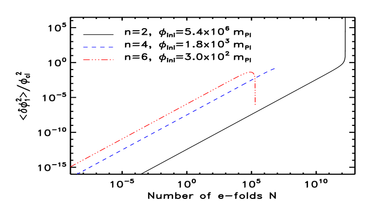
Figure 1: Evolution of $\left\langle\delta\varphi_{1}^{2}\right\rangle/\varphi_{\mathrm{cl}}^{2}$ versus the number of e-folds during inflation for three different chaotic potentials characterized by $n=2,4,6$. The initial values of the inflaton field corresponds to an initial energy density of $V_{\mathrm{in}}=0.5m_{{}_{\mathrm{P}l}}^{4}$ and implies that the total number of e-folds during inflation is not the same for the three models under considerations. This is also the reason why the curves do not stop at the same place. For the $n=2$ model, $\left\langle\delta\varphi_{1}^{2}\right\rangle$ always increases and, at some point, the perturbative scheme used to calculate it breaks down. For $n=4$, $\left\langle\delta\varphi_{1}^{2}\right\rangle/\varphi_{\mathrm{cl}}^{2}$ tends to a constant that is difficult to visualize because of the e-folds logarithmic scale. For $n\geq 6$, $\left\langle\delta\varphi_{1}^{2}\right\rangle$ possesses a maximum during inflation and then decreases.

Let us first consider the equation for $\delta\varphi_{1}$. If the initial conditions are such that $\delta\varphi_{1}(t={t_{\mathrm{in}}})=0$, then the solution reads

$$\delta\varphi_{1}(t)=\int_{t_{\mathrm{in}}}^{t}\kern-5.0pt\mathrm{d}\tau\frac{H^{3/2}(\varphi_{\rm cl})}{2\pi}\exp\!\left[-\int_{\tau}^{t}\kern-5.0pt\mathrm{d}\sigma\frac{2H^{\prime\prime}(\varphi_{\rm cl})}{\kappa}\right]\xi(\tau)\,.$$ (17)

This expression can be further simplified. If we use the classical equation of motion, then one can write the exponential term as

$$\exp\!\left(-\int_{\tau}^{t}\kern-5.0pt\mathrm{d}\sigma\frac{2H^{\prime\prime}}{\kappa}\right)=\exp\!\left[\int_{\varphi_{\rm cl}(\tau)}^{\varphi_{\rm cl}(t)}\kern-10.00002pt\mathrm{d}\varphi\frac{H^{\prime\prime}}{H^{\prime}}\right]=\frac{H^{\prime}\left[\varphi(t)\right]}{H^{\prime}\left[\varphi(\tau)\right]}\,.$$ (18)

Inserting the above expression into Eq. (17), one finally arrives at

$$\delta\varphi_{1}(t)=\frac{H^{\prime}\left[\varphi_{\rm cl}(t)\right]}{2\pi}\int_{t_{\mathrm{in}}}^{t}\kern-5.0pt\mathrm{d}\tau\frac{H^{3/2}\left[\varphi_{\rm cl}(\tau)\right]}{H^{\prime}\left[\varphi_{\rm cl}(\tau)\right]}\xi(\tau)\,.$$ (19)

We are now in a position where the various correlation functions can be calculated exactly. Since $\delta\varphi_{1}$ is linear in the noise $\xi$, the mean value obviously vanishes

$$\left\langle\delta\varphi_{1}\right\rangle=0\,.$$ (20)

Let us now evaluate the two-point correlation function calculated at the same time, i.e. the variance. Making use of Eq. (5), one obtains

$$\left\langle\delta\varphi_{1}^{2}\right\rangle=\frac{\kappa}{2}\left(\frac{H^{\prime}}{2\pi}\right)^{2}\!\!\int^{\varphi_{\mathrm{in}}}_{\varphi_{\rm cl}}\kern-6.99997pt\mathrm{d}\varphi\left(\frac{H}{H^{\prime}}\right)^{3}\,.$$ (21)

So far, the expressions presented above are general and do not rely on a particular shape of the inflaton potential. If we now specify the calculation to the chaotic potential given by Eq. (9), then the variance takes the form

$$\frac{\left\langle\delta\varphi_{1}^{2}\right\rangle}{m_{{}_{\mathrm{P}l}}^{2}}=-\frac{4}{3n}\frac{V(\varphi_{\mathrm{cl}})}{m_{{}_{\mathrm{P}l}}^{4}}\left(\frac{\varphi_{\rm cl}}{m_{{}_{\mathrm{P}l}}}\right)^{-2}\left[\left(\frac{\varphi_{\rm cl}}{m_{{}_{\mathrm{P}l}}}\right)^{4}-\left(\frac{\varphi_{\rm in}}{m_{{}_{\mathrm{P}l}}}\right)^{4}\right]\,.$$ (22)

Since $\varphi_{\rm cl}$ is always smaller than ${\varphi_{\mathrm{in}}}$ (because the field rolls down its potential), the above quantity is increasing with time and always positive as required.

We now turn to the equation of motion for the second order perturbation $\delta\varphi_{2}$. It can be solved by following exactly the steps that were described before. Then, the solution can be written as

$$\delta\varphi_{2}(t) = -\frac{H^{\prime}}{\kappa}\int_{t_{\mathrm{in}}}^{t}\kern-5.0pt\mathrm{d}\tau\frac{H^{\prime\prime\prime}}{H^{\prime}}\delta\varphi_{1}^{2}(\tau)$$ (23)

$$+\frac{3H^{\prime}}{4\pi}\int_{t_{\mathrm{in}}}^{t}\kern-5.0pt\mathrm{d}\tau H^{1/2}\delta\varphi_{1}(\tau)\xi(\tau)\,.$$

As expected the second order perturbation is quadratic in the noise. One can now easily evaluate the mean value of $\delta\varphi_{2}(t)$, taking into account a factor $1/2$ which originates from the fact that the Dirac $\delta$-function appearing in the noise correlation function is centered on an integration limit. One obtains

$$\frac{\left\langle\delta\varphi_{2}\right\rangle}{m_{{}_{\mathrm{P}l}}} = -\frac{n+2}{3n}\frac{V(\varphi_{\mathrm{cl}})}{m_{{}_{\mathrm{P}l}}^{4}}\left(\frac{\varphi_{\rm cl}}{m_{{}_{\mathrm{P}l}}}\right)^{-n/2-1}\left[\left(\frac{\varphi_{\rm cl}}{m_{{}_{\mathrm{P}l}}}\right)^{n/2+2}-\left(\frac{\varphi_{\rm in}}{m_{{}_{\mathrm{P}l}}}\right)^{n/2+2}\right]$$ (24)

$$+\frac{n-2}{3n}\frac{V(\varphi_{\mathrm{cl}})}{m_{{}_{\mathrm{P}l}}^{4}}\left(\frac{\varphi_{\rm in}}{m_{{}_{\mathrm{P}l}}}\right)^{4}\left(\frac{\varphi_{\rm cl}}{m_{{}_{\mathrm{P}l}}}\right)^{-n/2-1}\left[\left(\frac{\varphi_{\rm cl}}{m_{{}_{\mathrm{P}l}}}\right)^{n/2-2}-\left(\frac{\varphi_{\rm in}}{m_{{}_{\mathrm{P}l}}}\right)^{n/2-2}\right]\,.$$

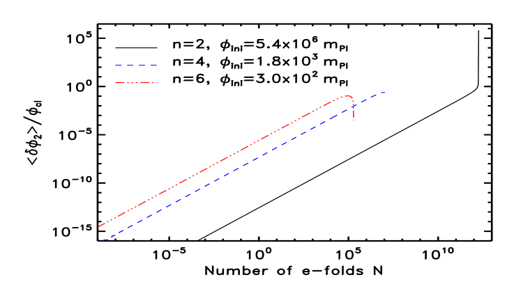
Figure 2: Evolution of $\left\langle\delta\varphi_{2}\right\rangle/\varphi_{\mathrm{cl}}$ with the number of e-folds during inflation for three different potentials. The initial values of the scalar field always correspond to an initial energy density of $V_{\mathrm{in}}=0.5m_{{}_{\mathrm{P}l}}^{4}$. As a consequence, the total number of e-folds during inflation is not the same in these three models and this explains why the three curves stop at different $N$. A value of $\left\langle\delta\varphi_{2}\right\rangle/\varphi_{\mathrm{cl}}$ greater than one signals a breakdown of the perturbative approach. For instance, this is the case for the $n=2$ model at the end of inflation.

The quantities $\left\langle\delta\varphi_{1}^{2}\right\rangle/\varphi_{\rm cl}^{2}$ and $\left\langle\delta\varphi_{2}\right\rangle/\varphi_{\rm cl}$ are represented in Fig. 1 and 2 for different potentials, i.e. for different values of the power index $n$. We find that for $n>4$ both quantities reach a maximum after an increasing phase, and then decrease to zero at late times, always remaining smaller than unity for any choice of the initial conditions (thus fully validating the perturbative treatment). Conversely, we see that their late time behavior is constant for $n=4$ or rapidly increasing for $n<4$, and appears in both cases to violate the validity of the perturbative approach for the extreme choice of an initial condition corresponding to an energy density near the Planck scale.

III.3 Classicalization

Let us study the late time behavior of $\left\langle\delta\varphi_{2}\right\rangle$, as given by Eq. (24), in more details. In this regime, one has $\varphi_{\mathrm{cl}}\ll\varphi_{\mathrm{in}}$. Then, it follows that

$$\frac{\left\langle\delta\varphi_{2}\right\rangle}{m_{{}_{\mathrm{P}l}}}\propto\left(\frac{\varphi_{\mathrm{cl}}}{m_{{}_{\mathrm{P}l}}}\right)^{n/2-1}\,.$$ (25)

From the above equation, one deduces that we have exact classicalization for the cases $n=2$ or $n=4$. Indeed, in this case, we have $\left\langle\varphi\right\rangle\simeq\varphi_{\mathrm{cl}}+\left\langle\delta\varphi_{2}\right\rangle\propto\varphi_{\mathrm{cl}}$ which is, by definition, what we mean by classicalization. For $n>4$, the situation is slightly different. In this case, $\left\langle\varphi\right\rangle$ is not exactly proportional to $\varphi_{\mathrm{cl}}$ but the extra contribution $\left\langle\delta\varphi_{2}\right\rangle$ decays faster than $\varphi_{\mathrm{cl}}$ and, hence, becomes negligible as can also be checked in Fig. 2. In this way, we also recover a classical behavior.

Let us now see what happens to a trajectory which is far from the mean value. From Eq. (22), it is easy to check that, at late times, we also have $\sqrt{\left\langle\delta\varphi_{1}^{2}\right\rangle}/m_{{}_{\mathrm{P}l}}\propto(\varphi_{\mathrm{cl}}/m_{{}_{\mathrm{P}l}})^{n/2-1}$ (a quantity which gives an estimate of the amplitude of the probability distribution). It follows than not only the mean value of the distribution but also its width evolves according to the classical solution.

Finally, the following remark is in order. The fact that the quantum effects are negligible does not mean that, at late times, the value of the quintessence field $\left\langle\varphi\right\rangle$ is the same as the corresponding classical field value calculated with the same initial conditions. Since the quantum could have accumulated in the early phase of evolution causing a deviation from the classical trajectory, this actually means that the late time value of $\left\langle\varphi\right\rangle$ can only be viewed as $\varphi_{\mathrm{cl}}$ but calculated with different initial conditions.

III.4 Comparison with Other Methods

In this section, we compare the results of the previous section with some known results of the literature.

In Refs. [25, 26], it has been shown that there is a case where the Langevin equation can be solved exactly. In order to permit a more direct comparison with those studies, we write the constant $V_{0}$ which appears in the expression of the potential (9) as $V_{0}/m_{{}_{\mathrm{P}l}}^{4}=3\lambda_{n}/(8\pi)$, i.e. in terms of the coupling constant $\lambda_{n}$. Then, the reasoning goes as follows. The Langevin equation can be written as

$$\frac{{\rm d}}{{\rm d}t}\left(\frac{\varphi}{m_{{}_{\mathrm{P}l}}}\right)+\frac{n\sqrt{\lambda_{n}}}{8\pi}m_{{}_{\rm Pl}}\left(\frac{\varphi}{m_{{}_{\mathrm{P}l}}}\right)^{n/2-1}$$

$$=\frac{\lambda_{n}^{3/4}}{2\pi}m_{{}_{\rm Pl}}^{1/2}\left(\frac{\varphi}{m_{{}_{\mathrm{P}l}}}\right)^{3n/4}\xi(t)\,.$$ (26)

There is an exact solution if $n=4$ because, in this case, the Langevin equation takes the form of a Bernoulli equation. The simplification comes from the fact that the equation can be put under the form of a linear equation for some power of the field (in the present context, this power is $-2$ hence the form of the next equation). Let us also notice that the choice $n=4/3$ would also lead to a Bernoulli equation but this case looks less interesting since the power index of the potential is no longer an integer. The Bernoulli equation can be solved exactly because it may be brought into a linear form by a change of variable. The solution can be written as

$$\left(\frac{\varphi}{m_{{}_{\mathrm{P}l}}}\right)^{-2} = {\rm e}^{\sqrt{\lambda_{4}}m_{{}_{\mathrm{P}l}}\left(t-t_{\rm in}\right)/\pi}\biggl{[}\left(\frac{\varphi_{\rm in}}{m_{{}_{\mathrm{P}l}}}\right)^{-2}-\frac{\lambda_{4}^{3/4}}{\pi}m_{{}_{\mathrm{P}l}}^{1/2}$$ (27)

$$\times\int_{t_{\rm in}}^{t}{\rm d}\tau\,{\rm e}^{-\sqrt{\lambda_{4}}m_{{}_{\mathrm{P}l}}\left(\tau-t_{\rm in}\right)/\pi}\xi(\tau)\biggr{]}\,.$$

Taking the inverse square root of the general solution one then obtains

$$\varphi(t)=\varphi_{\mathrm{cl}}(t)\left[1-\Psi(t)\right]^{-1/2}\,,$$ (28)

where $\varphi_{\mathrm{cl}}(t)$ is the classical solution that can be expressed explicitly in terms of cosmic time

$$\varphi_{\mathrm{cl}}(t)=\varphi_{\mathrm{in}}\exp\left[-\frac{\sqrt{\lambda_{4}}m_{{}_{\mathrm{P}l}}}{2\pi}\left(t-t_{\mathrm{in}}\right)\right],$$ (29)

while the quantity $\Psi(t)$ is defined by

$$\Psi(t)\equiv\frac{\lambda_{4}^{3/4}}{\pi}m_{{}_{\mathrm{P}l}}^{1/2}\int_{t_{\mathrm{in}}}^{t}{\rm d}\tau\left[\frac{\varphi_{\mathrm{cl}}(\tau)}{m_{{}_{\mathrm{P}l}}}\right]^{2}\xi(\tau)\,.$$ (30)

This function can be treated as a new dimensionless Gaussian noise with vanishing mean value and whose variance reads

$$\left\langle\Psi^{2}(t)\right\rangle=\frac{\lambda_{4}}{2\pi}\left[\left(\frac{\varphi_{\mathrm{in}}}{m_{{}_{\mathrm{P}l}}}\right)^{4}-\left(\frac{\varphi_{\mathrm{cl}}}{m_{{}_{\mathrm{P}l}}}\right)^{4}\right]\,.$$ (31)

We are now in a position where the various correlation functions of the scalar field can be computed. Here, we compute the two-point correlation function. Using Eq. (28), one gets

$$\left\langle\left(\frac{\varphi}{m_{{}_{\mathrm{P}l}}}\right)^{2}\right\rangle=\left(\frac{\varphi_{\rm cl}}{m_{{}_{\mathrm{P}l}}}\right)^{2}\sum_{k=0}^{+\infty}\left\langle\Psi^{k}\right\rangle\,.$$ (32)

Let us notice that we could have also computed any (i.e. $n$-point) correlation function of the field (including of course the mean value) using the same technique. Since we have to deal with a Gaussian process, only the even correlation function are non vanishing. In addition, for a Gaussian process we have $\left\langle\Psi^{2k}\right\rangle=(2k-1)!!\left\langle\Psi^{2}\right\rangle^{k}$. Therefore, we obtain a series the general term of which can be written as $2^{k}\Gamma\left(k+1/2\right)\left\langle\Psi^{2}\right\rangle^{k}/\sqrt{\pi}$, where we have used Eq. (8.339.2) of Ref. [27]. At this point two remarks are in order. Firstly, it is easy to convince oneself that the series (32) is in fact divergent. The interpretation of this fact is of course a little bit problematic but, on the other hand, it is well-known that perfectly well-defined distribution functions can have no moments. Below, we also give another interpretation of this fact. Secondly, looking at the expression of the new Gaussian noise $\Psi$, we see that the series is in fact an expansion in the coupling constant $\lambda_{4}$. Since this one is in fact tiny, one can try to work with the first term of the series only. Then, one obtains

$$\frac{\varphi}{m_{{}_{\mathrm{P}l}}} \simeq \frac{\varphi_{\rm cl}}{m_{{}_{\mathrm{P}l}}}\left[1+\frac{1}{2}\Psi(t)+\frac{3}{8}\Psi^{2}(t)+{\cal O}\left(\lambda_{4}^{9/4}\right)\right]\,.$$ (33)

This expression is in fact exactly similar to the one obtained previously for $\varphi_{\rm cl}(t)+\delta\varphi_{1}(t)+\delta\varphi_{2}(t)$ and therefore leads to the same correlation functions as before. It is easy to show that the expansion in the coupling constant is nothing but the expansion in the noise used before. Our method is more general because it is not restricted to the case $n=4$. This is because the expansion is directly performed in the Langevin equation rather than in its solution. The drawback of this last method is clearly that it is first necessary to find a solution of the Langevin equation, which is not an easy task, before the expansion can be taken. Let us emphasize again that, even if an exact solution is known, an expansion is still necessary because only some power of the field is generally obtained (in the present case $\varphi^{-2}$) and, in order to find the expression of the stochastic field itself, one should then compute the root of the solution.

The same conclusions can be obtained by means of a model where the random walk of the field is modified by the presence of a reflecting barrier. This model is explored in the Appendix A.

Another possibility studied in the literature is the use of the so-called scaling solutions, see Ref. [28]. Let us quickly review the method. The first step consists in rendering the stochastic process non multiplicative. This can be done by means of the transformation $x=16\times 3^{3/4}\pi^{4}\int_{-\infty}^{\varphi}V^{-3/4}(\theta){\rm d}\theta$ which reduces the Langevin equation to ${\rm d}x/{\rm d}t=-{\rm d}\tilde{V}/{\rm d}x+\xi(t)$ where $\tilde{V}=-3\times(4\pi^{2})^{5}/V[\varphi(x)]$. Explicitly, one has $-{\rm d}\tilde{V}/{\rm d}x=g\times(x/m_{{}_{\mathrm{P}l}})^{(n+4)/(3n-4)}$ where $g$ is a constant which depends on $V_{0}$ and $n$. The next step is to consider the time-dependent nonlinear transformation

$$\eta(x,t)=F^{-1}[{\rm e}^{-\gamma(t-{t_{\mathrm{in}}})}F(x)]\,,$$ (34)

where the function $F$ is defined by, see Ref. [28]

$$F(x) = \frac{x_{\rm in}}{m_{{}_{\mathrm{P}l}}}\exp\biggl{\{}\frac{\gamma(3n-4)}{2g(n-4)}\biggl{[}\left(\frac{x}{m_{{}_{\mathrm{P}l}}}\right)^{2(n-4)/(3n-4)}$$ (35)

$$-\left(\frac{x_{\rm in}}{m_{{}_{\mathrm{P}l}}}\right)^{2(n-4)/(3n-4)}\biggr{]}\biggr{\}}\,,$$

with $\gamma\equiv g(x_{\rm in}/m_{{}_{\mathrm{P}l}})^{2(4-n)/(3n-4)}$. Then, it is straightforward to show that the new stochastic process $\eta$ obeys the following equation

$$\frac{{\rm d}\eta}{{\rm d}t} = \biggl{[}1+2g\frac{n-4}{3n-4}(t-{t_{\mathrm{in}}})$$ (36)

$$\times\eta^{2(4-n)/(3n-4)}\biggr{]}^{-(n+4)/[2(n-4)]}\xi(t)\,.$$

So far, everything is exact. However, the above Langevin equation cannot be solved exactly. The so-called scaling solutions correspond to replacing $\eta$ by $\eta_{\rm cl}$ in the right hand side of Eq. (36). Then, clearly, the Langevin equation can be integrated in this approximation. Therefore, the scaling solutions are nothing but the result of an expansion in the noise and, again, are similar to the solutions found at the beginning of this section. We notice, as shown in Ref. [28], that the quantity $\eta_{\rm cl}$ is in fact a constant. This is consistent with the fact that this is the zeroth order solution (i.e. for which the noise term is simply neglected) of the above-mentioned expansion for which the Langevin equation simply reads ${\rm d}\eta/{\rm d}t=0$. Finally, in Ref. [28], a saddle point approximation is used in order to calculate the effective dispersion. The result found is, see Eq. (28) of Ref. [28]

$$\left\langle\varphi^{2}\right\rangle_{\rm eff} \propto H^{2}(\varphi_{\rm cl})\sinh\left[\ln H^{-4/n}(\varphi_{\rm cl})\right]$$ (37)

$$= \varphi^{n}\left(\varphi^{2}+\varphi^{-2}\right)\,,$$ (38)

which is exactly the result obtained in Eq. (22). This reinforces the result that the scaling solutions are very similar or even identical to the solutions exhibited here by means of the expansion in the noise term.

In conclusion, the solutions obtained previously for the stochastic inflaton are explicit and consistent with those already found in the literature. In the sequel, we use them as a description of the background in which the quintessence field lives.

IV Quintessence

IV.1 Classical Evolution

In order to explain the accelerated expansion of the universe, one postulates the presence of the quintessence field $Q$. This field is a test field during almost all the cosmic evolution and becomes dominant only recently when it drives the accelerated expansion. As is well-known for a scalar field, the equation of state $\omega_{Q}=p_{Q}/\rho_{Q}$ is time-dependent and, crucially, can be negative. The detailed evolution of $\omega_{Q}$ clearly depends on the shape of the quintessence potential $W(Q)$. An interesting choice is the inverse power law potential (with $\alpha>0$) which was first studied by Ratra and Peebles in Ref. [6]

$$W(Q)=W_{0}\left(\frac{Q}{m_{{}_{\mathrm{P}l}}}\right)^{-\alpha}.$$ (39)

During the radiation dominated era, it is possible to find an exact solution of the corresponding Klein Gordon equation for which $Q\propto a^{4/(\alpha+2)}$ or $\rho_{Q}\propto a^{-4\alpha/(\alpha+2)}$. This is also possible for the matter dominated era for which one has $Q\propto a^{3/(\alpha+2)}$ or $\rho_{Q}\propto a^{-3\alpha/(\alpha+2)}$. The two solutions we have just mentioned can also be expressed by means of the following equation [8]

$$\frac{{\rm d}^{2}W(Q)}{{\rm d}Q^{2}}=\frac{9}{2}\frac{\alpha+1}{\alpha}(1-\omega_{Q}^{2})H^{2}\,,$$ (40)

this expression being valid both during the radiation and matter dominated epochs. We can re-write the parameter $\omega_{Q}$ as $\omega_{Q}=(\alpha\omega_{{}_{\rm B}}-2)/(\alpha+2)$ where $\omega_{{}_{\rm B}}$ is the equation of state of the background, i.e. either $1/3$ or $0$. Since $\rho_{Q}$ redshifts slower than the background energy density, the scalar field contribution will eventually become dominant. From the above equation, it is easy to see that, when the quintessence field is about to dominate, its value is in fact of the order of the Planck mass. Then, the value of $W_{0}$ is constrained by the fact that the quintessence energy density is almost the critical energy density today. This gives

$$\frac{W_{0}}{m_{{}_{\mathrm{P}l}}^{4}}\simeq\frac{3}{8\pi}\frac{H_{0}^{2}}{m_{{}_{\mathrm{P}l}}^{2}}\,,$$ (41)

where $H_{0}$ is the Hubble parameter today, i.e. $H_{0}\simeq 10^{-61}m_{{}_{\mathrm{P}l}}$. Equipped with this relation, one can also estimate the ratio $W_{0}/V_{0}$ and one gets

$$\frac{W_{0}}{V_{0}}\simeq\frac{(4N_{*}+n)^{n/2+1}}{240\pi}\left(\frac{n}{16\pi}\right)^{n/2}\frac{H_{0}^{2}}{m_{{}_{\mathrm{P}l}}^{2}}\left(\frac{Q_{\rm rms-PS}}{T}\right)^{-2}\,.$$ (42)

This number is obviously extremely small, $\simeq{\cal O}(10^{-110})$.

The main property of the solutions described before is that they are attractors [6]. This means that there is no need to fine-tune the initial conditions and that the solution will be on tracks today for a large range of initial conditions. Let us be more precise about this particular point. Usually, one fixes the initial conditions at the end of inflation, at a redshift of $z=10^{28}$. Then, the allowed initial values for the energy density are approximatively such that [8, 10, 11]: $10^{-37}\mbox{GeV}^{4}\leq\rho_{Q}\leq 10^{61}\mbox{GeV}^{4}$ where $10^{-37}\mbox{GeV}^{4}$ is the background energy density at equality whereas $10^{61}\mbox{GeV}^{4}$ represents the background energy density (i.e. the radiation energy density) at the initial redshift. If, for instance, $\alpha=6$ and if the scalar field starts at rest, this means that the initial values of the field are such that $10^{-18}m_{{}_{\mathrm{P}l}}\leq Q_{\rm in}\leq 10^{-2}m_{{}_{\mathrm{P}l}}$ just after inflation. If $Q_{\rm in}$ is large initially, then the attractor is joined quite recently. Of course, the range of allowed initial conditions, when expressed in terms of the initial field, depends on the value of the parameter $\alpha$.

The values of $\alpha$ are constrained by the measurement of the equation of state today. The larger $\alpha$ is, the larger the equation of state parameter $\omega_{Q}$ is today. Since it is known that $\omega_{Q}$ cannot be too different from $-1$, this means that $\alpha$ cannot be too large. In fact, this conclusion rests on the particular shape of the Ratra-Peebles potential. From a model building point of view, it is more natural to consider the SUGRA potential given by [10, 11, 12, 13]

$$W(Q)=W_{0}{\rm e}^{4\pi Q^{2}/m_{{}_{\mathrm{P}l}}^{2}}\left(\frac{Q}{m_{{}_{\mathrm{P}l}}}\right)^{-\alpha}\,.$$ (43)

Then, the equation of state parameter today is modified. Since, today, the value of the field is of the order of the Planck mass, the supergravity exponential factor plays an important role in this regime. This has two consequences. Firstly, the equation of state is pushed toward the value $-1$ because the exponential factor increases the importance of the potential energy with respect to the kinetic energy. Secondly, the value of $\omega_{Q}$ becomes almost independent of $\alpha$ because, again, the exponential factor dominates. As a consequence the constraint on $\alpha$ can be relaxed and any value is in fact a priori possible. Moreover, in the very early universe, one has $Q\ll m_{{}_{\mathrm{P}l}}$ and, this time, the exponential factor becomes one. In this case, the SUGRA potential has the same shape as the Ratra-Peebles potential. In summary, if we have the SUGRA model in mind (which is, from a high-energy point of view, well-motivated), then, in the early universe, we can safely work with the Ratra-Peebles as an effective model (which is simpler, technically speaking) but without the usual restrictions on the parameter $\alpha$.

We have seen that the initial conditions are usually fixed just after inflation, at the beginning of the radiation dominated era. In this paper, we study the behavior of the quintessence field during the phase of inflation itself. One of our main goal is to check whether the behavior of $Q$ during inflation is compatible with the allowed initial conditions (in fact, “final” conditions from the point of view of the present study) described before. Clearly, if the final value of $Q$ (at the end of inflation) is not in the allowed range, then the quintessential scenario is in trouble. In fact, in order to avoid the above-mentioned situation, our study rather helps us to put constraints on the initial conditions, not at the beginning of the radiation dominated era as before, but at the beginning of the inflationary phase.

We start with a study of the classical evolution of the quintessence field (i.e. without the quantum effects). The classical quintessence field obeys the usual equation of motion for a scalar field in a FLRW background with the Hubble parameter depending on the classical inflaton field $\varphi_{\mathrm{cl}}$, namely

$${\ddot{Q}}_{\mathrm{cl}}+3H(\varphi_{\mathrm{cl}})\dot{Q}_{\mathrm{cl}}+W^{\prime}(Q_{\mathrm{cl}})=0\,.$$ (44)

Whenever the friction term is large, one can neglect the double derivative term, obtaining the standard slow-roll equation

$$\frac{{\rm d}Q_{\mathrm{cl}}}{{\rm d}t}+\frac{W^{\prime}(Q_{\mathrm{cl}})}{3H(\varphi_{\mathrm{cl}})}=0\,.$$ (45)

The consistency of this assumption can be directly checked. Taking the time derivative of the last equation one can actually show that

$$\frac{\ddot{Q}_{\mathrm{cl}}}{H(\varphi_{\mathrm{cl}})\dot{Q}_{\mathrm{cl}}}=-\frac{W^{\prime\prime}(Q_{\mathrm{cl}})}{3H^{2}(\varphi_{\mathrm{cl}})}+\epsilon,$$ (46)

where $\epsilon=-\dot{H}/H^{2}$ is the usual inflaton slow-roll parameter which is by assumption much smaller than $1$. Therefore, the slow roll approximation can be applied to the equations describing the motion of the quintessence field whenever the following condition is satisfied

$$\frac{W^{\prime\prime}(Q_{\mathrm{cl}})}{3H^{2}(\varphi_{\mathrm{cl}})}\ll 1\,.$$ (47)

If one applies this condition to the Ratra-Peebles potential, one arrives at

$$\left(\frac{Q_{\rm cl}}{m_{{}_{\mathrm{P}l}}}\right)^{\alpha+2}\gg\frac{\alpha(\alpha+1)W_{0}}{8\pi V(\varphi_{\mathrm{cl}})}\,.$$ (48)

Let us now turn to the solution of Eq. (45). For the Ratra-Peebles potential given by Eq. (39), the solution to this slow-roll equation can be expressed as

$$\frac{Q_{\rm cl}}{m_{{}_{\mathrm{P}l}}}=\left[\left(\frac{Q_{\mathrm{in}}}{m_{{}_{\mathrm{P}l}}}\right)^{\alpha+2}+\frac{\alpha(\alpha+2)W_{0}}{m_{{}_{\mathrm{P}l}}^{2}}\int^{\varphi_{\mathrm{in}}}_{\varphi_{\mathrm{cl}}(t)}\!\!\frac{\kern 0.0pt\mathrm{d}\chi}{V^{\prime}(\chi)}\right]^{1/(\alpha+2)}\,.$$ (49)

Using the chaotic inflationary potential (9) we get for any value of the power index such that $n>2$

$$\frac{Q_{\mathrm{cl}}}{m_{{}_{\mathrm{P}l}}}=\Biggl{\{}\left(\frac{Q_{\mathrm{in}}}{m_{{}_{\mathrm{P}l}}}\right)^{\alpha+2}+\frac{\alpha(\alpha+2)}{n(2-n)}\frac{W_{0}}{V_{0}}\\ \times\left[\left(\frac{\varphi_{\mathrm{in}}}{m_{{}_{\mathrm{P}l}}}\right)^{2-n}-\left(\frac{\varphi_{\mathrm{cl}}}{m_{{}_{\mathrm{P}l}}}\right)^{2-n}\right]\Biggr{\}}^{1/(\alpha+2)}\,,$$ (50)

while, for $n=2$, the result reads

$$\frac{Q_{\mathrm{cl}}}{m_{{}_{\mathrm{P}l}}}=\left[\left(\frac{Q_{\mathrm{in}}}{m_{{}_{\mathrm{P}l}}}\right)^{\alpha+2}+\frac{\alpha(\alpha+2)}{2}\frac{W_{0}}{V_{0}}\ln\frac{\varphi_{\mathrm{in}}}{\varphi_{\rm cl}(t)}\right]^{1/(\alpha+2)}.$$ (51)

These results are consistent with those obtained in Ref. [15]. The evolution of the quintessence field in the slow-roll regime for different initial values is plotted in Fig. 3.

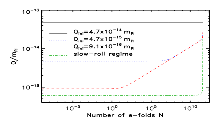
Figure 3: Classical evolution of the quintessence field for different initial conditions. A massive chaotic inflaton potential (i.e. $n=2$) has been assumed and the parameter $\alpha$ in the Ratra-Peebles potential has been taken to be equal to $6$. The initial condition for the inflaton field is such that $\varphi_{\mathrm{in}}=2.5\times 10^{6}m_{{}_{\mathrm{P}l}}$ corresponding to an initial energy density of $V_{\mathrm{in}}=0.1m_{{}_{\mathrm{P}l}}^{4}$. The green dotted-dashed line signals the limit of the slow-roll approximation. Below this line, the slow-roll approximation is no longer valid.

Let us quickly discuss these solutions. One can obtain a more compact expression if one notices that $\varphi_{\rm cl}\simeq\varphi_{\rm in}[1-N/(2N_{{}_{\rm T}})]$ where $N_{{}_{\rm T}}$ is the total number of e-folds during inflation. This expression is valid provided that $N<4\pi(\varphi_{\rm in}/m_{{}_{\mathrm{P}l}})^{2}/n=N_{{}_{\rm T}}+n/4\simeq N_{{}_{\rm T}}$. Then, one has

$$\frac{Q_{\mathrm{cl}}}{m_{{}_{\mathrm{P}l}}}\simeq\frac{Q_{\mathrm{in}}}{m_{{}_{\mathrm{P}l}}}\bigg{[}1+\frac{\alpha(\alpha+2)W_{0}}{2nV_{0}}\left(\frac{\varphi_{\mathrm{in}}}{m_{{}_{\mathrm{P}l}}}\right)^{2-n}\\ \times\left(\frac{Q_{\mathrm{in}}}{m_{{}_{\mathrm{P}l}}}\right)^{-\alpha-2}\frac{N}{N_{{}_{\rm T}}}\bigg{]}^{1/(\alpha+2)}\,.$$ (52)

If the initial value is large enough, then the dynamical term will remain negligible and the field is frozen until inflation ends. As a matter of fact, for any value of $n$ we obtain that $Q_{\mathrm{cl}}(t)\simeq Q_{\mathrm{in}}$ at all times if the initial value satisfies the constraint

$$\left(\frac{Q_{\mathrm{in}}}{m_{{}_{\mathrm{P}l}}}\right)^{\alpha+2}\gtrsim\left(\frac{W_{0}}{V_{0}}\right)\left(\frac{\varphi_{\mathrm{in}}}{m_{{}_{\mathrm{P}l}}}\right)^{2-n}\,.$$ (53)

If the above condition is satisfied at initial time, then, obviously, the condition given by Eq. (48) is also satisfied. There is also an intermediate regime for which the condition (53) is not satisfied but (48) is. In this case, the field is not frozen, even at initial times. Finally, if $Q_{\mathrm{in}}$ is sufficiently small so that the condition (48) is violated, then we expect the quintessence dynamics to rapidly bring back the field to the slow-roll regime, where the previous considerations apply.

IV.2 Perturbative Solutions

As mentioned at the beginning of this article, in order to study the evolution of the quintessence field, it is not sufficient to integrate the classical equation of motion since the quantum effects can play an important role and modify the classical evolution. We now analyze the stochastic behavior of the quintessence field, in the case where the total energy density is still dominated by the vacuum energy of the inflaton field. The stochastic evolution of the quintessence field $Q$ is controlled by a Langevin equation which, in the slow-roll approximation, reads

$$\frac{{\rm d}Q}{{\rm d}t}+\frac{W^{\prime}(Q)}{3H(\varphi)}=\frac{H^{3/2}(\varphi)}{2\pi}\xi_{Q}(t)\,,$$ (54)

where $\xi_{Q}$ is another white-noise field such that

$$\left\langle\xi_{Q}(t)\xi_{Q}(t^{\prime})\right\rangle=\delta(t-t^{\prime}),\quad\left\langle\xi_{Q}(t)\xi(t^{\prime})\right\rangle=0\,.$$ (55)

The solution of the Langevin equation (54) depends explicitly on $\xi_{Q}$ but also on the inflaton noise $\xi$ through the coarse-grained field $\varphi$.

In order to find an approximate solution to Eq. (54), one may try to use the same perturbative technique as the one used before for the inflaton field. Therefore, we expand the quintessence field about the classical slow-roll solution (49) and write

$$Q(t)=Q_{\rm cl}(t)+\delta Q_{1}+\delta Q_{2}+\cdots\,.$$ (56)

Then, it is easy to establish that the equations of motion for the perturbed quantities $\delta Q_{1}$ and $\delta Q_{2}$ are given by the following expressions

$$\frac{{\rm d}\delta Q_{1}}{{\rm d}t}+\frac{W^{\prime\prime}(Q_{\rm cl})}{3H(\varphi_{\rm cl})}\delta Q_{1} = \frac{W^{\prime}(Q_{\rm cl})H^{\prime}(\varphi_{\rm cl})}{3H^{2}(\varphi_{\rm cl})}\delta\varphi_{1}+\frac{H^{3/2}(\varphi_{\rm cl})}{2\pi}\xi_{Q}\,,$$ (57)

$$\frac{{\rm d}\delta Q_{2}}{{\rm d}t}+\frac{W^{\prime\prime}(Q_{\rm cl})}{3H(\varphi_{\rm cl})}\delta Q_{2} = \frac{W^{\prime}(Q_{\rm cl})H^{\prime}(\varphi_{\rm cl})}{3H^{2}(\varphi_{\rm cl})}\delta\varphi_{2}+\frac{W^{\prime}(Q_{\rm cl})H^{\prime\prime}(\varphi_{\rm cl})}{6H^{2}(\varphi_{\rm cl})}\delta\varphi_{1}^{2}-\frac{W^{\prime}(Q_{\rm cl})H^{\prime 2}(\varphi_{\rm cl})}{3H^{3}(\varphi_{\rm cl})}\delta\varphi_{1}^{2}$$ (58)

$$+\frac{W^{\prime\prime}(Q_{\rm cl})H^{\prime}(\varphi_{\rm cl})}{3H^{2}(\varphi_{\rm cl})}\delta\varphi_{1}\delta Q_{1}-\frac{W^{\prime\prime\prime}(Q_{\rm cl})}{6H(\varphi_{\rm cl})}\delta Q_{1}^{2}+\frac{3H^{1/2}(\varphi_{\rm cl})H^{\prime}(\varphi_{\rm cl})}{4\pi}\delta\varphi_{1}\xi_{Q}\,.$$

Although these equations look quite complicated, they can be solved easily because (by definition) they are linear. The solution for $\delta Q_{1}$ reads

$$\delta Q_{1}(t)=W^{\prime}(Q_{\rm cl})\int_{t_{\mathrm{in}}}^{t}\biggl{[}\frac{H^{\prime}(\varphi_{\rm cl})}{3H^{2}(\varphi_{\rm cl})}\delta\varphi_{1}(\tau)\\ +\frac{H^{3/2}(\varphi_{\rm cl})}{2\pi W^{\prime}(Q_{\rm cl})}\xi_{Q}(\tau)\biggr{]}{\rm d}\tau\,,$$ (59)

and, as required, is linear both in the quintessence noise $\xi_{Q}$ and (through $\delta\varphi_{1}$) in the inflaton noise $\xi$. As a consequence, $\delta Q_{1}$ has a vanishing mean value

$$\left\langle\delta Q_{1}\right\rangle=0\,,$$ (60)

but a non-vanishing variance given by the sum of two contributions originating from the inflaton and quintessence noise variances, namely

$$\left\langle\delta Q_{1}^{2}\right\rangle = \frac{W^{\prime 2}(Q_{\rm cl})}{9}\int_{t_{\mathrm{in}}}^{t}\int_{t_{\mathrm{in}}}^{t}\frac{H^{\prime}(\tau)}{H^{2}(\tau)}\frac{H^{\prime}(\eta)}{H^{2}(\eta)}\left\langle\delta\varphi_{1}(\tau)\delta\varphi_{1}(\eta)\right\rangle{\rm d}\tau{\rm d}\eta$$ (61)

$$+\frac{W^{\prime 2}(Q_{\rm cl})}{4\pi^{2}}\int_{t_{\mathrm{in}}}^{t}\int_{t_{\mathrm{in}}}^{t}\frac{H^{3/2}(\tau)}{W^{\prime}(\tau)}\frac{H^{3/2}(\eta)}{W^{\prime}(\eta)}\left\langle\xi_{Q}(\tau)\xi_{Q}(\eta)\right\rangle{\rm d}\tau{\rm d}\eta$$

$$\equiv \left\langle\delta Q_{1}^{2}\right\rangle|_{\xi_{\varphi}}+\left\langle\delta Q_{1}^{2}\right\rangle|_{\xi_{Q}}\,.$$ (62)

Let us notice that there is no mixed contribution since the cross-correlation $\left\langle\xi\xi_{Q}\right\rangle=0$. The detailed calculation of $\left\langle\delta Q_{1}^{2}\right\rangle$, in particular its explicit expression in terms of the inflaton field and/or the number of e-folds $N$, is rather lengthy and is carried out in the Appendix B.

Let us now turn to the second order correction. The solution for $\delta Q_{2}$ can be written as

$$\delta Q_{2}(t) = W^{\prime}(Q_{\rm cl})\int_{t_{\mathrm{in}}}^{t}\biggl{\{}\frac{H^{\prime}(\varphi_{\rm cl})}{3H^{2}(\varphi_{\rm cl})}\delta\varphi_{2}(\tau)+\left[\frac{H^{\prime\prime}(\varphi_{\rm cl})}{6H^{2}(\varphi_{\rm cl})}-\frac{H^{\prime 2}(\varphi_{\rm cl})}{3H^{3}(\varphi_{\rm cl})}\right]\delta\varphi_{1}^{2}(\tau)+\frac{W^{\prime\prime}(Q_{\rm cl})H^{\prime}(\varphi_{\rm cl})}{3W^{\prime}(Q_{\rm cl})H^{2}(\varphi_{\rm cl})}\delta\varphi_{1}(\tau)\delta Q_{1}(\tau)$$ (63)

$$-\frac{W^{\prime\prime\prime}(Q_{\rm cl})}{6W^{\prime}(Q_{\rm cl})H(\varphi_{\rm cl})}\delta Q_{1}^{2}(\tau)+\frac{3}{4\pi}\frac{H^{1/2}(\varphi_{\rm cl})H^{\prime}(\varphi_{\rm cl})}{W^{\prime}(Q_{\rm cl})}\delta\varphi_{1}(\tau)\xi_{Q}\biggr{\}}{\rm d}\tau\,.$$

As expected, one sees that $\delta Q_{2}$ is quadratic in the noises. From the above expression, one deduces that the mean value of $\delta Q_{2}$ is non-vanishing and is the sum of various terms

$$\left\langle\delta Q_{2}\right\rangle=\left\langle\delta Q_{2}\right\rangle|_{\delta\varphi_{2}}+\left\langle\delta Q_{2}\right\rangle|_{\delta\varphi_{1}^{2}}+\left\langle\delta Q_{2}\right\rangle|_{\delta\varphi_{1}\delta Q_{1}}+\left\langle\delta Q_{2}\right\rangle|_{\delta Q_{1}^{2}(\xi_{Q})}+\left\langle\delta Q_{2}\right\rangle|_{\delta Q_{1}^{2}(\xi_{\varphi})}\,,$$ (64)

where the last term in Eq. (63) does not contribute because

$$\left\langle\delta\varphi_{1}\xi_{Q}\right\rangle=0\,.$$ (65)

If we had not taken into account the stochastic behavior of the inflaton, only the term $\left\langle\delta Q_{2}\right\rangle|_{\delta Q_{1}^{2}(\xi_{Q})}$ would have contributed. Again, the explicit expressions of each term are given in the Appendix B.

Let us now quickly present what the outcome of the perturbative approach applied to the evolution of the quintessence field is. The main result is that when the classical evolution of the quintessence field is negligible, i.e. when the condition (53) holds, the variance reads

$$\left\langle\delta Q_{1}^{2}\right\rangle|_{\xi_{Q}}=\frac{16m_{{}_{\mathrm{P}l}}^{2}}{3n(n+2)}\frac{V_{0}}{m_{{}_{\mathrm{P}l}}^{4}}\left[\left(\frac{\varphi_{\mathrm{in}}}{m_{{}_{\mathrm{P}l}}}\right)^{n+2}-\left(\frac{\varphi_{\mathrm{cl}}}{m_{{}_{\mathrm{P}l}}}\right)^{n+2}\right]\,.$$ (66)

which is the same result already obtained in Ref. [15] that we recover here with a different method.

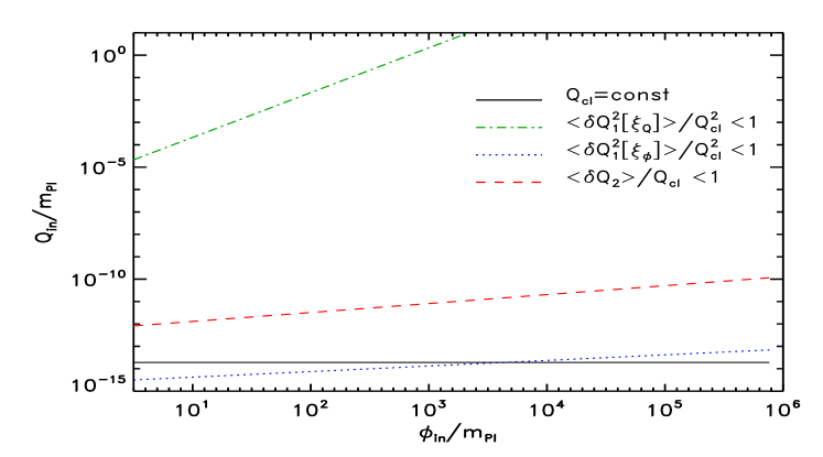
Figure 4: Constraints coming from the requirement that the perturbative approach is valid for the case $n=2$ and $\alpha=6$. The values of the initial conditions $\varphi_{\mathrm{in}}$ and $Q_{\mathrm{in}}$ are chosen such that the corresponding energy density is never Planckian, i.e. $V(\varphi_{\mathrm{in}})<m_{{}_{\mathrm{P}l}}^{4}$ and $V(Q_{\mathrm{in}})<m_{{}_{\mathrm{P}l}}^{4}$. Each line corresponds to a condition specified in the figure and that we describe below. By convention, the allowed region is always the region above the corresponding line. The solid black line indicates the regime where $Q_{\mathrm{cl}}$ can be considered as constant, see Eq. (53). The dot-dashed green line corresponds to the region where $\left\langle\delta Q_{1}^{2}\right\rangle/Q_{\mathrm{cl}}^{2}<1$, originating from the quintessence noise, is small, see Eq. (68). The dotted blue line corresponds to the same condition except that the variance now comes from the inflaton noise. Finally, the dashed red line corresponds to the condition $\left\langle\delta Q_{2}\right\rangle/Q_{\mathrm{cl}}<1$ where the mean value originates from the quintessence noise. As we have seen before, see Eq. (64), there are four other contributions but one can easily show that they do not lead to new constraints and this is the reason why they are not represented in this figure. As discussed in the text, the most stringent constraint comes from the requirement $\left\langle\delta Q_{1}^{2}\right\rangle/Q_{\mathrm{cl}}^{2}<1$.

Another general result that is established in details in the Appendix B is that, when the perturbative approach is valid, the contribution coming from the inflaton noise is completely negligible, see for instance Figs. 8.

Unfortunately, this is not a very strong argument because it is possible to see that the perturbative treatment is well under control only in a very small region of the parameter space. Indeed, one must check that the conditions

$$\frac{\left\langle\delta Q_{1}^{2}\right\rangle}{Q_{\mathrm{cl}}^{2}}\ll 1\,,\quad\frac{\left\langle\delta Q^{2}\right\rangle}{Q_{\mathrm{cl}}}\ll 1\,.$$ (67)

are fulfilled if one wants the perturbative approach to be valid. This leads to several constraints that are summarized in Fig. 4. More precisely, from Eq. (62), one sees that the first condition leads to two constraints while, looking at Eq. (64), one notices that the second one leads to fives constraints. As is apparent from Fig. 4, the most stringent constraint comes from the fact that the variance originating from the quintessence noise must be small in comparison with $Q_{\mathrm{cl}}^{2}$. Explicitly, working out this condition, it boils down to

$$\frac{Q_{\mathrm{in}}}{m_{{}_{\mathrm{P}l}}}\gtrsim\frac{\sqrt{V_{0}}}{m_{{}_{\mathrm{P}l}}^{2}}\left(\frac{\varphi_{\mathrm{in}}}{m_{{}_{\mathrm{P}l}}}\right)^{n/2+1}\,.$$ (68)

Let us also notice that this condition is a much more stringent condition than (53), see Fig. 4. For most values of $Q_{\mathrm{in}}$ and $\varphi_{\mathrm{in}}$, we rapidly get that $\left\langle\delta Q_{1}^{2}\right\rangle/Q_{\mathrm{cl}}^{2}\gg 1$, meaning that a large part of the initial condition space cannot be described by means of the perturbative approach. Therefore, there is the need for a different approach.

IV.3 The Reflecting Wall

The failure of the perturbative treatment is a signal of the fact that the classical evolution is not a good zeroth order solution for the perturbative expansion. The reason is that the equation of motion is dominated by the diffusive term due to the noise while the classical drift is in fact sub-dominant. It is therefore natural to neglect the classical term and to solve the approximate equation

$$\frac{{\rm d}Q}{{\rm d}t}=\frac{H^{3/2}(\varphi)}{2\pi}\xi\,.$$ (69)

The solution to this equation can be written as

$$Q=Q_{\mathrm{in}}+\int_{t_{\mathrm{in}}}^{t}\kern-5.0pt\mathrm{d}\tau\frac{H^{3/2}(\varphi)}{2\pi}\xi(\tau)\,.$$ (70)

As a first step, we also neglect the inflaton fluctuations and take $\varphi$ to be the classical field $\varphi_{\mathrm{cl}}$. As a consequence, $Q$ has a Gaussian probability distribution the mean of which is given by $\left\langle Q\right\rangle=Q_{\mathrm{in}}$ with a variance $\sigma_{Q}^{2}\equiv\left\langle Q^{2}\right\rangle-\left\langle Q\right\rangle^{2}$ which can be expressed as

$$\sigma_{Q}^{2}=\sigma_{0}^{2}(t)\equiv\int_{t_{\mathrm{in}}}^{t}\kern-5.0pt\mathrm{d}\tau\frac{H^{3}(\varphi_{\mathrm{cl}})}{4\pi^{2}}$$ (71)

$$= \frac{16m_{{}_{\mathrm{P}l}}^{2}}{3n(n+2)}\frac{V_{0}}{m_{{}_{\mathrm{P}l}}^{4}}\left[\left(\frac{\varphi_{\mathrm{in}}}{m_{{}_{\mathrm{P}l}}}\right)^{n+2}-\left(\frac{\varphi_{\mathrm{cl}}}{m_{{}_{\mathrm{P}l}}}\right)^{n+2}\right]\,.$$

One recognizes Eq. (66), first obtained in Ref. [15], and that we have re-derived in the preceding subsection by means of the perturbative approach. Here, we have shown that Eq. (66) can be valid even when the perturbative approach breaks down.

At this point a remark on the notation is in order. In the following $\sigma_{Q}^{2}$ always denotes the variance of the quintessence field while $\sigma_{0}^{2}$ is just a function defined by the above expression which turns out to be equal to $\sigma_{Q}^{2}$ in the situation where the classical drift and the inflaton noise are neglected.

The above model is in fact too simple for the following reason. The function $\sigma_{0}(t)$ increases with time and, at some point, is larger than $Q_{\mathrm{in}}$. In this case, there is a finite probability (tending to 50% at late times) that the quintessence field becomes negative. Clearly, this is not possible because, in this case, the classical term in the Langevin equation becomes dominant and prevents $Q$ to become negative. In other words, in this regime, the classical drift cannot be neglected. So, it seems that we are in fact back to the original problem which consists in solving exactly the full Langevin equation. However, there is a simple way out. Indeed, we can model the effect of the classical term by considering that there is a perfectly reflecting wall at $Q=0$ the purpose of which is of course to prevent the quintessence field to become negative. As discussed in Ref. [29], the probability distribution of a random walk is modified by a reflecting barrier in a way that is easy to estimate. Let us assume that we start with a normalized probability distribution for the variable $x$, $\int_{-\infty}^{+\infty}P(x){\rm d}x=1$. Then, let us put a reflecting wall at $x=a$ such that only the values $x>a$ are allowed. Then, Ref. [29] tells us that the new probability distribution is $P(x)+P(2a-x)$ and it is easy to check by mean of a simple change of variable that it is indeed normalized, i.e. $\int_{a}^{+\infty}[P(x)+P(2a-x)]{\rm d}x=1$. In the present context, we have $a=0$ and, hence, the resulting probability distribution becomes, for $Q>0$,

$$P(Q,t)=\frac{\mathrm{e}^{-(Q-Q_{\mathrm{in}})^{2}/(2\sigma_{0}^{2})}+\mathrm{e}^{-(Q+Q_{\mathrm{in}})^{2}/(2\sigma_{0}^{2})}}{\sqrt{2\pi}\sigma_{0}(t)}\,,$$ (72)

where $\sigma_{0}$ is given by Eq. (71) which means that, for the moment, the contribution coming from the inflaton noise is still neglected.

As mentioned before, the advantage of the reflecting wall model is that it permits simple analytical estimates of the relevant physical quantities. However, there is one feature of the model that is worth stressing here. The classical drift term which prevents the field to become negative depends on the parameter $\alpha$ but the wall, which is supposed to model this term, don’t. Therefore, one limitation of the reflecting wall model is that we have lost the $\alpha$-dependence of the result. Concretely, in the following, we will see that the mean value and/or the variance of $Q$ are $\alpha$ independent. Only an exact solution (or a numerical calculation) could allow us to test the accuracy of this assumption.

With the help of this probability distribution we can now calculate the mean and the variance of the quintessence field. For the mean, one obtains the following analytical expression

$$\left\langle Q\right\rangle=\sigma_{0}\left[\sqrt{\frac{2}{\pi}}\mathrm{e}^{-Q_{\mathrm{in}}^{2}/2\sigma_{0}^{2}}+\frac{Q_{\mathrm{in}}}{\sigma_{0}}\mathrm{Erf}\left(\frac{Q_{\mathrm{in}}}{\sqrt{2}\sigma_{0}}\right)\right]\,,$$ (73)

where $\mathrm{Erf}(z)$ is the error function defined by $\mathrm{Erf}(z)\equiv(2/\sqrt{\pi})\int_{0}^{z}{\rm d}t{\rm e}^{-t^{2}}$. To our knowledge, this explicit formula is new and has not been given elsewhere. In the same manner, one has $\left\langle Q^{2}\right\rangle=\sigma_{0}^{2}+Q_{\mathrm{in}}^{2}$ and, therefore, one has

$$\sigma_{Q}^{2}=\sigma_{0}^{2}+Q_{\mathrm{in}}^{2}-\left\langle Q\right\rangle^{2}\,,$$ (74)

where $\left\langle Q\right\rangle$ is given by Eq. (73). One notices the variance of the quintessence field $\sigma_{Q}^{2}$ is now different from the function $\sigma_{0}^{2}$, $\sigma_{Q}^{2}\neq\sigma_{0}^{2}$. Let us emphasize again that the above results are not subject to the limitations of the perturbative approach. In particular, the difference between the classical value and the quantum (or stochastic) average needs not to be small.

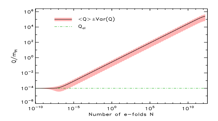
Figure 5: Evolution of $\left\langle Q\right\rangle$ (solid black line) calculated from Eq. (73) (but with the inflaton noise taken into account) and compared with the corresponding classical evolution (dotted-dashed green line) $Q_{\mathrm{cl}}$. The dashed area represents the zone $\pm\sigma$ around the mean value where $\sigma$ has been obtained with the help of Eq. (81). The difference between $\left\langle Q\right\rangle$ and $Q_{\mathrm{cl}}$ at the end of inflation can be many orders of magnitude (and is, in the present case, of about $8$ orders of magnitude) demonstrating that it is crucial to take into account the quantum effects during inflation. The curves have been obtained for a massive chaotic model, i.e. $n=2$ and for the Ratra-Peebles potential with $\alpha=6$. The initial value of the inflaton is $\varphi_{\mathrm{in}}=5.4\times 10^{6}m_{{}_{\mathrm{P}l}}$ corresponding to an initial energy density of $V_{\mathrm{in}}=0.5\times m_{{}_{\mathrm{P}l}}^{4}$. The initial value of the quintessence field is $Q_{\mathrm{in}}=10^{-4}m_{{}_{\mathrm{P}l}}$ corresponding to $W_{\mathrm{in}}=1.25\times 10^{-99}m_{{}_{\mathrm{P}l}}^{4}$.

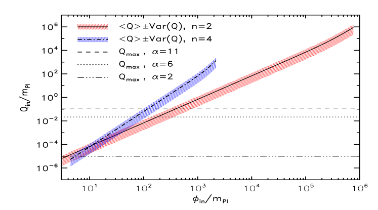
Figure 6: The quantity $\left\langle Q\right\rangle$ at the end of inflation versus the initial value of the inflaton field calculated according to Eq. (83) for two chaotic models, $n=2$ and $n=4$. As noticed in the text, $\left\langle Q\right\rangle$ at the end of inflation does not depend on the initial value of the quintessence field because there is an attractor solution given by Eq. (76). The fact that the final value does not depend on the parameter $\alpha$ is due to the description of the classical drift term by means of the reflecting wall. The two curves start and stop at different values of the initial inflaton field because the minimal value (defined to be the one which leads to at least $60$ e-folds) and the maximal value (defined to be the one which corresponds to $V_{\mathrm{in}}=m_{{}_{\mathrm{P}l}}^{4}$) are not the same according to the model (i.e. $n$) under considerations (for instance, $\varphi_{\mathrm{in}}=3.1m_{{}_{\mathrm{P}l}}$ for $n=2$ while $\varphi_{\mathrm{in}}=4.4m_{{}_{\mathrm{P}l}}$ for $n=4$). The horizontal lines represent the maximal values of $\left\langle Q\right\rangle$ (for different values of the index $\alpha$) at the end of inflation such that the attractor is joined today. These values are computed by means of Eq. (85).

If we insert Eq. (71) into Eqs. (73) and (74), one obtains the mean value $\left\langle Q\right\rangle$ and the variance $\sigma_{Q}^{2}$ as functions of the inflaton and/or the number of e-folds. At initial time, one has $\sigma_{0}\rightarrow 0$ and therefore $\left\langle Q\right\rangle\rightarrow Q_{\mathrm{in}}$, where we have used the fact that $\mathrm{Erf}(z)\rightarrow 1$ when $z\rightarrow+\infty$. For the variance, one has in the same regime (i.e. initially for $\varphi\rightarrow\varphi_{\mathrm{in}}$ and $\sigma_{0}(t)\ll Q_{\mathrm{in}}$)

$$\sigma_{Q}^{2}\rightarrow\sigma_{0}^{2}(t)\,,$$ (75)

where we have used Eq. (74) and the behavior of the mean at initial times. This means that, in this regime, we recover the previous results obtained by means of the perturbative approach.

One can also study what happens at late times when $\sigma_{0}(t)\gg Q_{\mathrm{in}}$. In this case, one has

$$\left\langle Q\right\rangle\rightarrow\sqrt{\frac{2}{\pi}}\sigma_{0}(t)\,.$$ (76)

The situation is reminiscent to the behavior of quintessence in the more traditional situation where the background evolution is dominated either by radiation or matter. Indeed, as it is the case in this well-studied context and as explained before, the late time evolution of $\left\langle Q\right\rangle$ is independent on the initial conditions, i.e. on $Q_{\mathrm{in}}$. In other words, there is an attractor for $\left\langle Q\right\rangle$ given by Eq. (76). In this situation, the final value of the quintessence field only depends on the initial value of the inflaton field (and, of course, on which kind of potential is responsible for inflation: in the present context, it only depends on $n$). However, this conclusion should be toned down because we will see in the following that another quantity of interest, namely the probability that the quintessence field be on tracks today (or, equivalently, that its value at the end of inflation be in a given range) does depend on $Q_{\mathrm{in}}$ (and, in fact, also on $\varphi_{\mathrm{in}}$).

Using the above expression, the variance of the quintessence field at late times can also be estimated. It is given by

$$\sigma_{Q}^{2}\rightarrow\left(1-\frac{2}{\pi}\right)\sigma_{0}^{2}(t)\,.$$ (77)

We see that, as $\sigma_{0}(t)$ increases and as the probability that the random-walking field is reflected by the wall becomes non negligible, the mean value $\left\langle Q\right\rangle$ is shifted toward higher values while its variance slightly shrinks.

We are now in a position where we can come back to one of our starting questions, namely the influence of the inflaton noise. In particular, we study whether including the inflaton fluctuations can cause significant deviations from the above results and, if so, under which physical conditions this is the case. In order to take into account this effect, we re-start from Eq. (70). In this formula, the argument of the Hubble parameter is no longer the classical inflaton but the stochastic process studied in the previous section. Then, one can use the perturbative treatment studied before but, and this is of course the crucial point, only for the inflaton field. Indeed, we have seen before that this perturbative treatment (contrary to the perturbative treatment for the quintessence field) is almost always reliable. Performing a Taylor expansion of Eq. (70), one obtains

$$Q = Q_{\mathrm{in}}+\frac{1}{2\pi}\int_{t_{\mathrm{in}}}^{t}\kern-5.0pt\mathrm{d}\tau\biggl{\{}H^{3/2}(\varphi_{\rm cl})+\frac{3}{2}H^{\prime}(\varphi_{\rm cl})H^{1/2}(\varphi_{\rm cl})\delta\varphi_{1}(\tau)+\frac{3}{2}H^{\prime}(\varphi_{\rm cl})H^{1/2}(\varphi_{\rm cl})\delta\varphi_{2}(\tau)$$ (78)

$$+\frac{1}{2}\biggl{[}\frac{3}{2}H^{\prime\prime}(\varphi_{\rm cl})H^{1/2}(\varphi_{\rm cl})+\frac{3}{4}H^{\prime 2}(\varphi_{\rm cl})H^{-1/2}(\varphi_{\rm cl})\biggr{]}\delta\varphi_{1}^{2}(\tau)+\cdots\biggr{\}}\xi(\tau)\,.$$

Equipped with this solution, one can now reintroduce the reflecting wall and recalculate the various moments. Clearly, since the solution is still linear in the quintessence noise, the probability function of the quintessence field, taking into account the wall, is still given by Eq. (72) but, in the expression of $P(Q,t)$, $\sigma_{0}$ should now be replaced by another function (of the classical inflaton noise or of the number of e-folds) that, in the following, we simply denote by $\sigma$ (not to be confused with $\sigma_{Q}$). The replacement of $\sigma_{0}$ by $\sigma$ is the only change needed. Otherwise the expression of the new $P(Q,t)$ is similar to the one given by Eq. (72). Let us now determine $\sigma$ explicitly. As before, $\sigma$ is simply given by the variance deduced from Eq. (78) using the fact that we have white noises. Eq. (78) implies that $\sigma^{2}$ is given by

$$\sigma^{2}(t)=\int_{t_{\mathrm{in}}}^{t}\kern-5.0pt\mathrm{d}\tau\frac{\left\langle H^{3}(\varphi)\right\rangle}{4\pi^{2}}\,,$$ (79)

where the mean value in the integral can be expressed through a power expansion of $H^{3}(\varphi)$ up to second order about its classical value yielding

$$\left\langle H^{3}(\varphi)\right\rangle=H^{3}(\varphi_{\mathrm{cl}})+3H^{2}H^{\prime}\left\langle\delta\varphi_{2}\right\rangle\\ +3\left[H(H^{\prime})^{2}+\frac{H^{2}H^{\prime\prime}}{2}\right]\left\langle\delta\varphi_{1}^{2}\right\rangle\,,$$ (80)

that can now be easily integrated. The final result is

$$\sigma^{2}(t) = \sigma_{0}^{2}(t)+\frac{16m_{{}_{\mathrm{P}l}}^{2}}{3n}\frac{V_{0}^{2}}{m_{{}_{\mathrm{P}l}}^{8}}\Biggl{\{}\frac{4}{3n}\left(\frac{\varphi_{\mathrm{in}}}{m_{{}_{\mathrm{P}l}}}\right)^{n/2+2}\left[\left(\frac{\varphi_{\mathrm{in}}}{m_{{}_{\mathrm{P}l}}}\right)^{3n/2}-\left(\frac{\varphi_{\mathrm{cl}}}{m_{{}_{\mathrm{P}l}}}\right)^{3n/2}\right]+\left(\frac{\varphi_{\mathrm{in}}}{m_{{}_{\mathrm{P}l}}}\right)^{4}\left[\left(\frac{\varphi_{\mathrm{in}}}{m_{{}_{\mathrm{P}l}}}\right)^{2n-2}-\left(\frac{\varphi_{\mathrm{cl}}}{m_{{}_{\mathrm{P}l}}}\right)^{2n-2}\right]$$ (81)

$$-\frac{n}{n+1}\left[\left(\frac{\varphi_{\mathrm{in}}}{m_{{}_{\mathrm{P}l}}}\right)^{2n+2}-\left(\frac{\varphi_{\mathrm{cl}}}{m_{{}_{\mathrm{P}l}}}\right)^{2n+2}\right]\Biggr{\}}\,$$

Let us now compare the function $\sigma(N)$ with the function $\sigma_{0}(N)$. At early times, i.e. when $\varphi_{\mathrm{cl}}(t)\sim\varphi_{\mathrm{in}}$, a linearization is sufficient in order to obtain a good approximation (and this is in fact the case for a large part of inflation). A striking feature of the above result is that the extra term coming from the inflaton quantum fluctuations cancel out, the first non-vanishing contribution being of order $\mathcal{O}[(N/N_{{}_{\rm T}})^{2}]$, where we remind that $N_{{}_{\rm T}}$ is the total number of e-folds. Therefore, for the main part of the inflationary era we can safely consider that $\sigma(t)\simeq\sigma_{0}(t)$. Again, we reach the conclusion that the effects originating from the inflaton noise do not play a crucial role. Conversely, at late times, when $\varphi_{\mathrm{cl}}(t)\ll\varphi_{\mathrm{in}}$, the above expression yields

$$\sigma^{2}(t)=\sigma_{0}^{2}(t)\left[1+\frac{(n+2)(7n+4)}{3n(n+1)}\frac{V_{\mathrm{in}}}{m_{{}_{\mathrm{P}l}}^{4}}\right]\,,$$ (82)

meaning that, as could be expected, the contribution of the inflaton quantum fluctuations is significant only when inflation starts near the Planck scale, while it becomes negligible for smaller values of the initial energy density.

We are now in a position where one can compute the new mean and variance exactly. As already mentioned, the new probability function is given by Eq. (72) with $\sigma_{0}$ replaced by $\sigma$. This immediately means that $\left\langle Q\right\rangle$ and $\sigma_{Q}^{2}$ are given by Eqs. (73) and (74) with $\sigma_{0}$ replaced by $\sigma$. The evolution of $\left\langle Q\right\rangle$ versus the number of e-folds is displayed in Fig. 5. At initial times, one has $\left\langle Q\right\rangle\simeq Q_{\mathrm{in}}$ and $\sigma_{Q}^{2}\simeq\sigma^{2}\simeq\sigma_{0}^{2}$, the last approximate equality coming from the property established before Eq. (82). On the other hand, the mean value and the variance of the quintessence field at late times read (if the initial condition for the inflaton field is large enough in order to reach the regime where $\sigma\gg Q_{\mathrm{in}}$)

$$\left\langle Q\right\rangle=\sqrt{\frac{2}{\pi}}\;\sigma\,,\quad\sigma_{Q}=\sqrt{1-\frac{2}{\pi}}\;\sigma$$ (83)

where in the above equations $\sigma$ is the $\sigma(t)$ calculated at the end of inflation, which is given by

$$\sigma=\varphi_{\mathrm{in}}\sqrt{\frac{16}{3n(n+2)}\frac{V_{\rm in}}{m_{{}_{\mathrm{P}l}}^{4}}\left[1+\frac{(n+2)(7n+4)}{3n(n+1)}\frac{V_{\mathrm{in}}}{m_{{}_{\mathrm{P}l}}^{4}}\right]}\,,$$ (84)

where we have used Eq. (82) and an approximation for $\sigma_{0}$ valid at late times. One notices that the two quantities of Eq. (83) growing function of $\varphi_{\mathrm{in}}$. This can be checked explicitly in Fig. 6 where the final values of $\left\langle Q\right\rangle$ versus $\varphi_{\mathrm{in}}$ are represented.

There is another important consequence that can be deduced from what has been discussed so far. As already mentioned, the energy density of the quintessence field at the beginning of the radiation era (i.e. at the end of inflation) must be such that $10^{-113}m_{{}_{\mathrm{P}l}}^{4}<\rho_{Q}<10^{-9}m_{{}_{\mathrm{P}l}}^{4}$ if one wants $Q$ to be on tracks today. Assuming for simplicity that the field starts at rest, this implies

$$\frac{Q_{\rm min}}{m_{{}_{\mathrm{P}l}}}\equiv 10^{-107/\alpha}<\frac{Q}{m_{{}_{\mathrm{P}l}}}<10^{-9/\alpha}\equiv\frac{Q_{\rm max}}{m_{{}_{\mathrm{P}l}}}\,.$$ (85)

Since, during inflation, $Q$ is a stochastic quantity, one can study the probability for a given model (that is to say for a given choice of the power indices and of the initial conditions $Q_{\mathrm{in}}$ and $\varphi_{\mathrm{in}}$) that the field is in the appropriate range. This probability allows us to evaluate the likelihood of the various models under considerations, rejecting those for which this quantity is small. In this way, we can thus constrain the value of the initial conditions for the fields and exclude a portion of the parameter space. Two remarks are in order here. Firstly, as is clear from Eq. (72), the probability will depend on $Q_{\mathrm{in}}$. Therefore, although the late time evolution of $\left\langle Q\right\rangle$ is independent of $Q_{\mathrm{in}}$, this dependence is reintroduced via the calculation of the probabilities. Secondly, the result will also depend on $\varphi_{\mathrm{in}}$. As a consequence, for a fixed value of $n$ and $\alpha$, one can hope to derive constraints on the initial value of the quintessence field but also on the total number of e-folds during inflation.

A given model will be accepted if a large part of its probability distribution calculated at the end of inflation is contained within the allowed range. A rough estimate of this constraint can be obtained by simply requiring that the mean value of the distribution falls in this range within one square root of the variance. Using the previous results of this section, one finds that imposing that $\left\langle Q\right\rangle\pm\sigma_{Q}$ falls between $Q_{\rm min}$ and $Q_{\rm max}$ yields

$$Q_{\rm min}<\left(\sqrt{\frac{2}{\pi}}\pm\sqrt{1-\frac{2}{\pi}}\right)\sigma<Q_{\rm max}\,.$$ (86)

Therefore, in order to obtain a probability of order one must have that $\sigma\lesssim Q_{\rm max}$. This implies an upper bound on $\varphi_{\mathrm{in}}$ that can be roughly estimated to (neglecting the contribution from inflaton fluctuations)

$$\frac{\varphi_{\mathrm{in}}}{m_{{}_{\mathrm{P}l}}}\lesssim\left(\frac{m_{{}_{\mathrm{P}l}}^{2}}{\sqrt{V_{0}}}\frac{Q_{\rm max}}{m_{{}_{\mathrm{P}l}}}\right)^{2/(n+2)}\sim 10^{10(\alpha-2)/[\alpha(n+2)]}\,.$$ (87)

It is easy to see from the above formula that this constraint is quite stringent. Let us also notice that this also a constraint on the total number of e-folds during inflation, very roughly speaking $N_{{}_{\rm T}}\lesssim 10^{20(\alpha-2)/[\alpha(n+2)]}$.

More precisely, if one uses the probability density function given by Eq. (72) (with, as already discussed at length, $\sigma_{0}$ replaced by $\sigma$ if one wants to take into account the inflaton noise at the end of inflation), one can calculate the exact probability for the quintessence to be on tracks today. One arrives at

$$P(Q_{\rm min}<Q<Q_{\rm max}|Q_{\mathrm{in}},\alpha,\phi_{\mathrm{in}},n) = \frac{1}{2}\biggl{[}{\rm Erf}\left(\frac{Q_{\rm max}-Q_{\mathrm{in}}}{\sqrt{2}\sigma}\right)-{\rm Erf}\left(\frac{Q_{\rm min}-Q_{\mathrm{in}}}{\sqrt{2}\sigma}\right)+{\rm Erf}\left(\frac{Q_{\rm max}+Q_{\mathrm{in}}}{\sqrt{2}\sigma}\right)$$ (88)

$$-{\rm Erf}\left(\frac{Q_{\rm min}+Q_{\mathrm{in}}}{\sqrt{2}\sigma}\right)\biggr{]}\,.$$

\psfrag{!}{\!\!/}\includegraphics[width=203.80193pt,height=173.44534pt]{proba_alpha2.eps}

\psfrag{!}{\!\!/}\includegraphics[width=203.80193pt,height=173.44534pt]{contour_alpha2.eps}

\psfrag{!}{\!\!/}\includegraphics[width=203.80193pt,height=173.44534pt]{proba_alpha6.eps}

\psfrag{!}{\!\!/}\includegraphics[width=203.80193pt,height=173.44534pt]{contour_alpha6.eps}

\psfrag{!}{\!\!/}\includegraphics[width=203.80193pt,height=173.44534pt]{proba_alpha11.eps}

\psfrag{!}{\!\!/}\includegraphics[width=203.80193pt,height=173.44534pt]{contour_alpha11.eps}

Figure 7: Probability computed from Eq. (88) that the quintessence field is on tracks today for various models with $n=2$ and different power indices $\alpha$ (from top to bottom, $\alpha=2,6,11$). For all the models under consideration, the maximum allowed value of the initial inflaton is $\varphi_{\mathrm{in}}=7.6\times 10^{5}m_{{}_{\mathrm{P}l}}$ (coming from the fact that $V_{\mathrm{in}}<m_{{}_{\mathrm{P}l}}^{4}$). From the plots, one notices that values larger than $27m_{{}_{\mathrm{P}l}}$, $1.3\times 10^{3}m_{{}_{\mathrm{P}l}}$ and $3.0\times 10^{3}m_{{}_{\mathrm{P}l}}$ respectively (corresponding to an initial energy density $V_{\mathrm{in}}$ of $1.3\times 10^{-9}m_{{}_{\mathrm{P}l}}^{4}$, $2.9\times 10^{-6}m_{{}_{\mathrm{P}l}}^{4}$ and $1.5\times 10^{-5}m_{{}_{\mathrm{P}l}}^{4}$) are excluded at $99\%$ CL. One also notices that, since the confidence region enlarges for increasing values of $\alpha$, large values of the power index $\alpha$ are statistically preferred.

The detailed behavior of this probability as a function of the initial conditions $\varphi_{\mathrm{in}}$ and $Q_{\mathrm{in}}$ is shown in Fig. 7 for $n=2$ and different power indices $\alpha$. We see that a large portion of the parameter space can be excluded. Actually, for $n=2$, the largest allowed initial condition is $\varphi_{\mathrm{in}}\simeq 7.6\times 10^{5}m_{{}_{\mathrm{P}l}}$, corresponding to the Planck energy density. However, at $99\%$ of confidence level, initial values larger than $27m_{{}_{\mathrm{P}l}}$ ($\alpha=2$), $1.3\times 10^{3}m_{{}_{\mathrm{P}l}}$ ($\alpha=6$) or $3.0\times 10^{3}m_{{}_{\mathrm{P}l}}$ ($\alpha=11$) are excluded. This also shows that, since the confidence region enlarges with the power index $\alpha$, large values of $\alpha$ are statistically more favored than small values.

V Discussion and Conclusions

In this section, we briefly discuss other aspects of the question studied in this article and present our conclusions.

In the preceding sections, we have calculated the evolution of the quintessence field during inflaton taking into account the quantum effects. What about these quantum effects in the subsequent cosmological eras? After the reheating, during the radiation and matter dominated phases, it is easy to show that the quintessence field evolves classically starting from the value reached at the end of inflation and determined by its random walk during inflation. Indeed, since the noise in the Langevin equation is controlled by the quantum fluctuations of the modes leaving the horizon, it rapidly becomes negligible as the accelerated expansion stops and the modes start to reenter the horizon.

However, a new phase of accelerated expansion driven by the quintessence field is now taking place and, clearly, the above argument does not apply in this case. Therefore, one may wonder whether the influence of the quantum effects should not be taken into account when one computes the evolution of $Q$ at present time. This could have important observational consequences, in particular if the stochastic behavior of $Q$ modifies the value of the equation of state. However, it is easy to demonstrate that this is not so. The problem is in fact very similar to calculating the evolution of the inflaton field during inflation since, at present time, the quintessence field is no longer a test field but actually determines the evolution of the background. Therefore, even though the slow roll approximation might not be so satisfactory in this case, we can at least estimate the relevance of these late stochastic fluctuations by simply setting $n=-\alpha$ into Eq. (22) (since, in some sense, the Ratra-Peebles potential is nothing but an inflationary chaotic potential with a negative index). This equation, provided one substitutes $\varphi_{\mathrm{cl}}$ with $Q_{\mathrm{cl}}$ and $V(\varphi_{\mathrm{cl}})$ with $W(Q_{\mathrm{cl}})$, should be a reasonable estimate of $\left\langle\delta Q^{2}\right\rangle/Q^{2}$. Since the quintessence field is now on the attractor, its value must be of the order of the Planck mass. In addition, it is slowly rolling down its potential toward higher values. As a consequence, from Eq. (22), one gets the following rough estimate

$$\frac{\left\langle\delta Q^{2}\right\rangle}{Q^{2}}\bigg{|}_{\mathrm{now}}\lesssim\frac{W(Q_{\rm now})}{m_{{}_{\mathrm{P}l}}^{4}}\simeq 10^{-123}\,,$$ (89)

meaning that any stochastic deviation from the classical trajectory is completely negligible at present time.

Let us now end this work by reviewing what are the main conclusions of our study. The main result is that, taking into account the quantum effects during inflation is important since the stochastic diffusion term dominates over the classical drift term and that, as a consequence, the value of $\left\langle Q\right\rangle$ can differ from $Q_{\mathrm{cl}}$ by several orders of magnitude. For the first time to our knowledge, we have given an analytical estimate describing the evolution of $\left\langle Q\right\rangle$ during inflation, see Eq. (73).

Another new result is the fact that, requiring the quintessence field to have a large probability to be on tracks today, allows us to put quite stringent constraints on the initial conditions $Q_{\mathrm{in}}$ and $\varphi_{\mathrm{in}}$. Typically, the quintessence field must start from small values. We have also established that large values of $\alpha$ are favored (we notice in passing that, if we consider the Ratra-Peebles potential only and not the SUGRA one, the same conclusion is reached from the constraints that exist on the equation of state today). Another interesting result is that the inflaton field must also start from quite small values. This implies that the total number of e-folds during inflation is also limited. On the other hand, we have remarked the existence of an attractor for $\left\langle Q\right\rangle$, see Eq. (76), due to the fact that the final value of $\left\langle Q\right\rangle$ is independent of $Q_{\mathrm{in}}$. However, a dependence in the initial conditions is reintroduced in the calculation of the probability which has allowed us to put the constraints mentioned just before.

One of the main purpose of our paper was also to study the influence of the inflaton noise on the evolution of the quintessence field. The approximation consisting in neglecting the inflaton fluctuations has been shown to be justified in most cases, basically because the corresponding contributions to the mean value and/or to the variance are proportional to $V_{\mathrm{in}}/m_{{}_{\mathrm{P}l}}^{4}$, see for instance Eq. (83). Even in the extreme case of Planckian initial conditions for the inflaton field (i.e. $V_{\mathrm{in}}\sim m_{{}_{\mathrm{P}l}}^{4}$), the inflaton noise is unlikely to modify $\left\langle Q\right\rangle/m_{{}_{\mathrm{P}l}}$ by more than one order of magnitude compared to what is obtained taking into account the quintessence noise only.

It is also interesting to compare these results to those obtained in the paper [15] which was the first to take into account the quantum effects in the calculation of the evolution of $\left\langle Q\right\rangle$. Basically, our findings confirm and/or justify the results of Ref. [15] and somewhat extend their validity. We have recovered the same equation for the variance and our new equation (73) for the mean value of $Q$ confirms the conclusions that can be drawn from the figures of Ref. [15], namely that the quantum effects can play an important role during inflation. In Ref. [15], the inflaton noise has not been considered and, as mentioned above, we have demonstrated that this is, in most cases, a good approximation.

Finally, let us describe some questions that are left unanswered and some possible improvements to the present study. In order to be able to find analytical solutions, we have modeled the classical drift term with a reflecting wall. The price to pay is that we have lost the dependence in the parameter $\alpha$. The drift term acts differently for different Ratra-Peebles potentials while the wall repels the field regardless to $\alpha$. Although we do not expect a strong dependence, it would be interesting to quantify this effect. The problem is that, if one includes the exact classical term, then the Langevin equation is no longer analytically solvable. The only way out seems to numerically integrate this equation. However, even this solution could be difficult because a term like $Q^{-\alpha}$ can rapidly become very large and, hence, problematic from the numerical point of view.

Another interesting question would be to study what happens when one considers the case of a colored noise since it is clear that a white noise is not, physically, the most relevant case. Concretely, this amounts to replace the Heaviside function in the expansion of the field by a smooth function and, in principle, this could affect the evolution of the quintessence field during inflation although, again, we do not expect a very important effect.

For the moment, we postpone the study of all the issues to future works.

Acknowledgments

We wish to thank S. Matarrese for many enlightening comments and discussions.

Appendix A Reflecting Wall for the Inflaton

Another way to look at the quantum evolution of the inflaton is the following. From Eq. (31), it is clear that the variance of $\Psi(t)$ is a growing function of time. However, in order for the solution of Eq. (28) to be defined we need to impose the condition $\Psi(t)<1$. Otherwise, this equation is clearly meaningless and, of course, if this condition is not satisfied, the series of Eq. (33) is not convergent. This is probably the reason for the problems encountered before. The above condition can be thought of as constraining the random walk of $\Psi$ with a reflecting wall. As explained in the preceding section, see also Ref. [29], the resulting probability distribution for $\Psi$ with the wall located at $\Psi=1$ is given by

$$P(\Psi,t)=\frac{{\rm e}^{-\Psi^{2}/\left(2\left\langle\Psi^{2}\right\rangle\right)}+{\rm e}^{-(\Psi-2)^{2}/\left(2\left\langle\Psi^{2}\right\rangle\right)}}{\sqrt{2\pi\left\langle\Psi^{2}(t)\right\rangle}}\,,$$ (90)

and the corresponding probability distribution for $\varphi$, obtained via the relation $P[\varphi,t]=P[\Psi(\varphi),t]|{\rm d}\Psi/{\rm d}\varphi|$, becomes

$$P(\varphi,t)=P\left[\Psi(\varphi)\right]\frac{2}{\varphi_{\mathrm{cl}}}\left(\frac{\varphi_{\mathrm{cl}}}{\varphi}\right)^{3}\,.$$ (91)

This probability distribution has a finite mean value that can be expressed as [this equation can also be obtained by using the link between $\Psi$ and $\varphi$ given by Eq. (28) and the probability distribution of $\Psi$ given by Eq. (90)]

$$\left\langle\varphi\right\rangle=\varphi_{\mathrm{cl}}\frac{{\rm e}^{-1/\left(4\left\langle\Psi^{2}\right\rangle\right)}}{\sqrt{\left\langle\Psi^{2}\right\rangle}}\sqrt{\frac{\pi}{2}}I_{-1/4}\!\!\left(\frac{1}{4\left\langle\Psi^{2}\right\rangle}\right),$$ (92)

where $I_{\nu}(x)$ is the modified Bessel function of the first kind. For small values of $\left\langle\Psi^{2}\right\rangle$, the mean value reads

$$\left\langle\varphi\right\rangle=\varphi_{\mathrm{cl}}\left[1+\frac{3}{8}\left\langle\Psi^{2}\right\rangle+\mathcal{O}\left(\left\langle\Psi^{2}\right\rangle^{2}\right)\right],$$ (93)

yielding therefore the same results as (33). Let also notice that all higher moments are divergent in accordance with the discussion presented in the section on the evolution of the inflaton field.

Appendix B Perturbative solution for the quintessence field

B.1 Solution at First Order

In this appendix, we present the explicit expressions (as a function of the classical inflaton field and/or of the number of e-folds) of $\left\langle\delta Q_{1}^{2}\right\rangle$ given by Eqs. (61) and (62) and of $\left\langle\delta Q_{2}\right\rangle$ given by Eq. (64). We start with Eq. (62) which is the sum of two terms. In order to evaluate the first term coming from the inflaton noise, i.e. $\left\langle\delta Q_{1}^{2}\right\rangle|_{\xi_{\varphi}}$, one must calculate the two-point correlation function of $\delta\varphi_{1}$. Using the solution of Eq. (19), one obtains

$$\left\langle\delta\varphi_{1}(\tau)\delta\varphi_{1}(\eta)\right\rangle=\frac{1}{4\pi^{2}}H^{\prime}(\tau)H^{\prime}(\eta)\left[\int_{t_{\mathrm{in}}}^{\eta}\frac{H^{3}(\sigma)}{H^{\prime 2}(\sigma)}{\rm d}\sigma+\Theta(\eta-\tau)\int_{\eta}^{\tau}\frac{H^{3}(\sigma)}{H^{\prime 2}(\sigma)}{\rm d}\sigma\right]\,.$$ (94)

In the above expression, $\Theta(z)$ is the Heaviside function, i.e. is zero if $z<0$ and one otherwise. Then, using the link between the cosmic time and the classical inflaton field in the slow-roll approximation, the remaining integrations can be easily performed since they just boil down to integrating power-law functions. One obtains

$$\frac{\left\langle\delta Q_{1}^{2}\right\rangle}{m_{{}_{\mathrm{P}l}}^{2}}\biggl{|}_{\xi_{\varphi}} = \frac{4\alpha^{2}}{3n^{2}}\frac{W_{0}}{V_{0}}\frac{W_{0}}{m_{{}_{\mathrm{P}l}}^{4}}\left(\frac{Q_{\mathrm{cl}}}{m_{{}_{\mathrm{P}l}}}\right)^{-2\alpha-2}\Biggl{\{}\frac{1}{8-n}\left[\left(\frac{\varphi_{\mathrm{cl}}}{m_{{}_{\mathrm{P}l}}}\right)^{-n/2}-\left(\frac{\varphi_{\rm in}}{m_{{}_{\mathrm{P}l}}}\right)^{-n/2}\right]\times\left[\left(\frac{\varphi_{\mathrm{cl}}}{m_{{}_{\mathrm{P}l}}}\right)^{-n/2+4}-\left(\frac{\varphi_{\rm in}}{m_{{}_{\mathrm{P}l}}}\right)^{-n/2+4}\right]$$ (95)

$$+\frac{1}{n}\left(\frac{\varphi_{\rm in}}{m_{{}_{\mathrm{P}l}}}\right)^{4}\left[\left(\frac{\varphi_{\mathrm{cl}}}{m_{{}_{\mathrm{P}l}}}\right)^{-n/2}-\left(\frac{\varphi_{\rm in}}{m_{{}_{\mathrm{P}l}}}\right)^{-n/2}\right]\times\left[\left(\frac{\varphi_{\mathrm{cl}}}{m_{{}_{\mathrm{P}l}}}\right)^{-n/2}-\left(\frac{\varphi_{\rm in}}{m_{{}_{\mathrm{P}l}}}\right)^{-n/2}\right]$$

$$-\frac{4}{(4-n)(8-n)}\left[\left(\frac{\varphi_{\mathrm{cl}}}{m_{{}_{\mathrm{P}l}}}\right)^{4-n}-\left(\frac{\varphi_{\rm in}}{m_{{}_{\mathrm{P}l}}}\right)^{4-n}\right]-\frac{1}{8-n}\left(\frac{\varphi_{\rm in}}{m_{{}_{\mathrm{P}l}}}\right)^{-n/2+4}\left[\left(\frac{\varphi_{\mathrm{cl}}}{m_{{}_{\mathrm{P}l}}}\right)^{-n/2}-\left(\frac{\varphi_{\rm in}}{m_{{}_{\mathrm{P}l}}}\right)^{-n/2}\right]$$

$$+\frac{1}{8-n}\left(\frac{\varphi_{\rm in}}{m_{{}_{\mathrm{P}l}}}\right)^{-n/2}\left[\left(\frac{\varphi_{\mathrm{cl}}}{m_{{}_{\mathrm{P}l}}}\right)^{-n/2+4}-\left(\frac{\varphi_{\rm in}}{m_{{}_{\mathrm{P}l}}}\right)^{-n/2+4}\right]\Biggr{\}}\,.$$

The evolution of $\left\langle\delta Q_{1}^{2}\right\rangle|_{\xi_{\varphi}}$ as a function of the number of e-folds is displayed in Fig. 8. The main feature of this formula is that it is proportional to $(W_{0}/V_{0})\times(W_{0}/m_{{}_{\mathrm{P}l}}^{4})$ which is, as discussed before, very small. This is confirmed by the plot, see the left panel in Fig. 8.

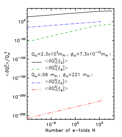
Figure 8: Left panel: evolution of $\langle\delta Q_{1}^{2}\rangle/Q_{\mathrm{cl}}^{2}$ calculated in the perturbative regime for two different set of initial conditions (i.e. two different values of $\varphi_{\mathrm{in}}$ and $Q_{\mathrm{in}}$) and for a model with $n=2$ and $\alpha=6$. For each set of initial conditions specified explicitly in the figure, the contribution coming from the quintessence noise and the contribution originating from the inflaton noise are represented. The perturbative treatment is under control only in the case $\varphi_{\mathrm{in}}=221m_{{}_{\mathrm{P}l}}$ and $Q_{\mathrm{in}}=0.06m_{{}_{\mathrm{P}l}}$ corresponding to initial energy densities given by $V_{\mathrm{in}}=3.7\times 10^{-8}m_{{}_{\mathrm{P}l}}^{4}$ and $W_{\mathrm{in}}=2.8\times 10^{-114}m_{{}_{\mathrm{P}l}}^{4}$ (since all the corresponding curves lie in the region $\langle\delta Q_{1}^{2}\rangle/Q_{\mathrm{cl}}^{2}<1$). The plot demonstrates clearly that, in the perturbative regime, the inflaton noise is totally negligible. Right panel: evolution of $\langle\delta Q_{2}\rangle/Q_{\mathrm{cl}}$ for the initial conditions $\varphi_{\mathrm{in}}=221m_{{}_{\mathrm{P}l}}$ and $Q_{\mathrm{in}}=0.06m_{{}_{\mathrm{P}l}}$. The five curves correspond to the five contributions of Eq. (64). Again, it is obvious that the four contributions originating from the inflaton noise are unimportant.

Let us now turn to the term sourced only by the quintessence noise. Using the fact that the quintessence noise is white the second term of Eq. (61) becomes

$$\left\langle\delta Q_{1}^{2}\right\rangle|_{\xi_{Q}}=\frac{W^{\prime 2}(Q_{\rm cl})}{4\pi^{2}}\!\!\int_{t_{\mathrm{in}}}^{t}\kern-5.0pt\mathrm{d}\tau\frac{H^{3}(\varphi_{\rm cl})}{W^{\prime 2}(Q_{\rm cl})},$$ (96)

Then, using the expression of the inflaton and quintessence potentials, straightforward calculations lead to the following formula in terms of hypergeometric functions

$$\frac{\left\langle\delta Q_{1}^{2}\right\rangle}{m_{{}_{\mathrm{P}l}}^{2}}\biggl{|}_{\xi_{Q}} = \frac{16}{3n(2-n)\mu}\frac{V_{0}}{m_{{}_{\mathrm{P}l}}^{4}}\left(\frac{Q_{\mathrm{cl}}}{Q_{\rm in}}\right)^{-2\alpha-2}\times\Delta^{-\nu}$$ (97)

$$\times \Biggl{\{}\left(\frac{\varphi_{\mathrm{cl}}}{m_{{}_{\mathrm{P}l}}}\right)^{\mu(n-2)}{}_{2}F_{1}\left[\nu,\mu,\mu+1,\frac{\Delta(\varphi_{\rm in}/m_{{}_{\mathrm{P}l}})^{2-n}-1}{\Delta}\left(\frac{\varphi_{\mathrm{cl}}}{m_{{}_{\mathrm{P}l}}}\right)^{n-2}\right]$$

$$- \left(\frac{\varphi_{\rm in}}{m_{{}_{\mathrm{P}l}}}\right)^{\mu(n-2)}{}_{2}F_{1}\left[\nu,\mu,\mu+1,\frac{\Delta(\varphi_{\rm in}/m_{{}_{\mathrm{P}l}})^{2-n}-1}{\Delta}\left(\frac{\varphi_{\rm in}}{m_{{}_{\mathrm{P}l}}}\right)^{n-2}\right]\Biggr{\}}\,,$$

where we have used the definitions

$$\mu\equiv\frac{n+2}{n-2}-\frac{2(\alpha+1)}{\alpha+2}\,,\quad\nu\equiv-\frac{2(\alpha+1)}{\alpha+2}\,,\quad\Delta\equiv\frac{\alpha(\alpha+2)}{n(n-2)}\Upsilon\,,\quad\Upsilon\equiv\frac{W_{0}}{V_{0}}\left(\frac{m_{{}_{\mathrm{P}l}}}{Q_{\rm in}}\right)^{\alpha+2}\,,$$ (98)

and where we have assumed that $n\neq 2$. The number $\mu$ is always positive for $n\leq 6$ which is the case we are mostly interested in and the number $\nu$ is, on the contrary, always negative. The evolution of $\left\langle\delta Q_{1}^{2}\right\rangle|_{\xi_{Q}}$ is represented in Fig. 8. The presence of the hypergeometric functions is linked to the fact that the classical quintessence field is not totally frozen. Looking at Eq. (50), one sees that the term responsible for the slight evolution of $Q_{\mathrm{cl}}$ is in fact proportional to $\Delta$. Indeed, in the limit $\Delta\rightarrow 0$, or equivalently $\Upsilon\rightarrow 0$, the classical quintessence field becomes $Q=Q_{\rm in}$, i.e. is actually frozen. In this case, one has

$${}_{2}F_{1}\left[\nu,\mu,\mu+1,\frac{\Delta(\varphi_{\rm in}/m_{{}_{\mathrm{P}l}})^{2-n}-1}{\Delta}\left(\frac{\varphi_{\mathrm{cl}}}{m_{{}_{\mathrm{P}l}}}\right)^{n-2}\right]\rightarrow\left(\frac{\varphi_{\mathrm{cl}}}{m_{{}_{\mathrm{P}l}}}\right)^{-\nu(n-2)}\Delta^{\nu}\frac{\mu}{\mu-\nu}\,,$$ (99)

and Eq. (97) reads

$$\frac{\left\langle\delta Q_{1}^{2}\right\rangle}{m_{{}_{\mathrm{P}l}}^{2}}\biggl{|}_{\xi_{Q}}\rightarrow\frac{16}{3n(n+2)}\frac{V_{0}}{m_{{}_{\mathrm{P}l}}^{4}}\left[\left(\frac{\varphi_{\rm ini}}{m_{{}_{\mathrm{P}l}}}\right)^{n+2}-\left(\frac{\varphi_{\mathrm{cl}}}{m_{{}_{\mathrm{P}l}}}\right)^{n+2}\right]\,,$$ (100)

which is exactly the expression derived in Ref. [15]. This term is proportional to the factor $V_{0}/m_{{}_{\mathrm{P}l}}^{4}$ which is much larger than $(W_{0}/V_{0})\times(W_{0}/m_{{}_{\mathrm{P}l}}^{4})$. As a result, we expect the term originating from the quintessence noise to dominate over the term originating from the inflaton noise and, as already mentioned, this conclusion is confirmed by the plots in Fig. 8. A priori this conclusion is valid only in the regime where the above expressions have been established, i.e. in the perturbative regime.

We have noticed before that the solution expressed in terms of the hypergeometric function is valid provided $n\neq 2$. The case $n=2$, for which the evolution of the classical quintessence field is given by Eq. (51), requires a special treatment. In this case, one finds

$$\frac{\left\langle\delta Q_{1}^{2}\right\rangle}{m_{{}_{\mathrm{P}l}}^{2}}\biggl{|}_{\xi_{Q}} = \frac{16}{3\times 8}\frac{V_{0}}{m_{{}_{\mathrm{P}l}}^{4}}\left(\frac{Q_{\mathrm{cl}}}{Q_{\rm in}}\right)^{-2\alpha-2}\left(\frac{\varphi_{\rm in}}{m_{{}_{\mathrm{P}l}}}\right)^{4}\left[\frac{8}{\alpha(\alpha+2)\Upsilon}\right]^{\nu}\exp\left[\frac{8}{\alpha(\alpha+2)\Upsilon}\right]$$ (101)

$$\times \left\{\gamma\left[\frac{3\alpha+4}{\alpha+2},\frac{8}{\alpha(\alpha+2)\Upsilon}-4\ln\frac{\varphi_{\mathrm{cl}}}{\varphi_{\rm in}}\right]-\gamma\left[\frac{3\alpha+4}{\alpha+2},\frac{8}{\alpha(\alpha+2)\Upsilon}\right]\right\}\,,$$

where $\gamma(\beta,x)$ is the incomplete gamma function defined by

$$\gamma(\beta,x)\equiv\int_{0}^{x}{\rm e}^{-t}t^{\beta-1}{\rm d}t\,.$$ (102)

In the limit $\Upsilon\rightarrow 0$, using the formula $\gamma(\beta,x)\simeq\Gamma(\beta)-x^{\beta-1}{\rm e}^{-x}$ when $x\rightarrow 0$, one obtains

$$\frac{\left\langle\delta Q_{1}^{2}\right\rangle}{m_{{}_{\mathrm{P}l}}^{2}}\biggl{|}_{\xi_{Q}}\rightarrow\frac{16}{3\times 8}\frac{V_{0}}{m_{{}_{\mathrm{P}l}}^{4}}\left[\left(\frac{\varphi_{\rm ini}}{m_{{}_{\mathrm{P}l}}}\right)^{4}-\left(\frac{\varphi}{m_{{}_{\mathrm{P}l}}}\right)^{4}\right]\,,$$ (103)

which is again the expression found in Ref. [15], specialized to the case $n=2$. The previous conclusion, namely that this term dominates the contribution coming from the inflaton noise, is not modify in this particular case.

B.2 Solution at Second Order

We now turn to the calculation of the mean value of $\delta Q_{2}$ given by the sum of five contributions as can be seen in Eq. (64). In principle, the calculations of these five terms can be performed in the general case, where the classical quintessence field in given either by Eq. (50) or Eq. (51). However, for simplicity, we give only the expressions corresponding to the case where $Q_{\mathrm{cl}}$ is frozen, i.e. to the limit $\Upsilon\rightarrow 0$. In this case, all the integrations become trivial since they only involve integrals of power-law functions. The first term, $\left\langle\delta Q_{2}\right\rangle|_{\delta\varphi_{2}}$, originates from the term $\delta\varphi_{2}$ only. It is given by

$$\frac{\left\langle\delta Q_{2}\right\rangle}{m_{{}_{\mathrm{P}l}}}\biggl{|}_{\delta\varphi_{2}} = -\frac{\alpha}{12n}\frac{W_{0}}{m_{{}_{\mathrm{P}l}}^{4}}\left(\frac{Q_{\rm in}}{m_{{}_{\mathrm{P}l}}}\right)^{-\alpha-1}\Biggl{\{}(n+2)\left[\left(\frac{\varphi_{\mathrm{cl}}}{m_{{}_{\mathrm{P}l}}}\right)^{2}-\left(\frac{\varphi_{\rm in}}{m_{{}_{\mathrm{P}l}}}\right)^{2}\right]+(n-2)\left(\frac{\varphi_{\rm in}}{m_{{}_{\mathrm{P}l}}}\right)^{4}\left[\left(\frac{\varphi_{\mathrm{cl}}}{m_{{}_{\mathrm{P}l}}}\right)^{-2}-\left(\frac{\varphi_{\rm in}}{m_{{}_{\mathrm{P}l}}}\right)^{-2}\right]$$ (104)

$$+\frac{16}{n}\left(\frac{\varphi_{\rm in}}{m_{{}_{\mathrm{P}l}}}\right)^{n/2+2}\left[\left(\frac{\varphi_{\mathrm{cl}}}{m_{{}_{\mathrm{P}l}}}\right)^{-n/2}-\left(\frac{\varphi_{\rm in}}{m_{{}_{\mathrm{P}l}}}\right)^{-n/2}\right]\Biggr{\}}\,,$$

The main feature of the above term is the presence of the overall factor $W_{0}/m_{{}_{\mathrm{P}l}}^{4}\times\left(Q_{\mathrm{in}}/m_{{}_{\mathrm{P}l}}\right)^{-\alpha-1}$ (of course, the powers of the inflaton field can also play a role but for a crude order of magnitude estimate, one can ignore them). The second term participating to the expression of $\left\langle\delta Q_{2}\right\rangle$ comes from $\delta\varphi_{1}^{2}$. It is given by

$$\frac{\left\langle\delta Q_{2}\right\rangle}{m_{{}_{\mathrm{P}l}}}\biggl{|}_{\delta\varphi_{1}^{2}}=\frac{\alpha(n+2)}{12n}\frac{W_{0}}{m_{{}_{\mathrm{P}l}}^{4}}\left(\frac{Q_{\rm in}}{m_{{}_{\mathrm{P}l}}}\right)^{-\alpha-1}\Biggl{\{}\left[\left(\frac{\varphi_{\mathrm{cl}}}{m_{{}_{\mathrm{P}l}}}\right)^{2}-\left(\frac{\varphi_{\rm in}}{m_{{}_{\mathrm{P}l}}}\right)^{2}\right]+\left(\frac{\varphi_{\rm in}}{m_{{}_{\mathrm{P}l}}}\right)^{4}\left[\left(\frac{\varphi_{\mathrm{cl}}}{m_{{}_{\mathrm{P}l}}}\right)^{-2}-\left(\frac{\varphi_{\rm in}}{m_{{}_{\mathrm{P}l}}}\right)^{-2}\right]\Biggr{\}}\,.$$ (105)

We see that this term also scales as $W_{0}/m_{{}_{\mathrm{P}l}}^{4}\times\left(Q_{\mathrm{in}}/m_{{}_{\mathrm{P}l}}\right)^{-\alpha-1}$. Therefore, we expect the previous contribution and this term to be of the same order of magnitude. This can be checked explicitly in Fig. 8. The third term comes from $\delta\varphi_{1}\delta Q_{1}$ where it should be understood that, in $\delta Q_{1}$, only the term proportional to the inflaton noise matters. One obtains

$$\frac{\left\langle\delta Q_{2}\right\rangle}{m_{{}_{\mathrm{P}l}}}\biggl{|}_{\delta\varphi_{1}\delta Q_{1}}=-\frac{2\alpha^{2}(\alpha+1)}{3n^{2}}\frac{W_{0}}{m_{{}_{\mathrm{P}l}}^{4}}\frac{W_{0}}{V_{0}}\left(\frac{Q_{\rm in}}{m_{{}_{\mathrm{P}l}}}\right)^{-2\alpha-3}\Biggl{\{}\frac{1}{n}\left(\frac{\varphi_{\rm in}}{m_{{}_{\mathrm{P}l}}}\right)^{4}\left[\left(\frac{\varphi_{\mathrm{cl}}}{m_{{}_{\mathrm{P}l}}}\right)^{-n}-\left(\frac{\varphi_{\rm in}}{m_{{}_{\mathrm{P}l}}}\right)^{-n}\right]$$

$$-\frac{16}{n(8-n)}\left(\frac{\varphi_{\rm in}}{m_{{}_{\mathrm{P}l}}}\right)^{-n/2+4}\left[\left(\frac{\varphi_{\mathrm{cl}}}{m_{{}_{\mathrm{P}l}}}\right)^{-n/2}-\left(\frac{\varphi_{\rm in}}{m_{{}_{\mathrm{P}l}}}\right)^{-n/2}\right]-\frac{n}{(4-n)(8-n)}\left[\left(\frac{\varphi_{\mathrm{cl}}}{m_{{}_{\mathrm{P}l}}}\right)^{-n+4}-\left(\frac{\varphi_{\rm in}}{m_{{}_{\mathrm{P}l}}}\right)^{-n+4}\right]\Biggr{\}}\,,$$ (106)

In comparison with the two previous terms, we see that there is an extra overall factor equal to $W_{0}/V_{0}\times\left(Q_{\mathrm{in}}/m_{{}_{\mathrm{P}l}}\right)^{-\alpha-2}$. As a consequence, this term is expected to be sub-dominant with respect to the two previous contributions and, again, this can be checked explicitly in Fig. 8. Of course, one could try to compensate the smallness of $W_{0}/V_{0}$ by a large value of $\left(Q_{\mathrm{in}}/m_{{}_{\mathrm{P}l}}\right)^{-\alpha-2}$, i.e. by a large value of the index $\alpha$ but this would lead to very artificial, hence unphysical, models. Then, the fourth term, originating from the term $\delta Q_{1}^{2}(\xi_{Q})$, can be written as

$$\frac{\left\langle\delta Q_{2}\right\rangle}{m_{{}_{\mathrm{P}l}}}\biggl{|}_{\delta Q_{1}^{2}(\xi_{Q})} = \frac{8\alpha(\alpha+1)(\alpha+2)}{3n^{2}(n+2)}\frac{V_{0}}{m_{{}_{\mathrm{P}l}}^{4}}\frac{W_{0}}{V_{0}}\left(\frac{Q_{\rm in}}{m_{{}_{\mathrm{P}l}}}\right)^{-\alpha-3}\Biggl{\{}\frac{1}{4}\left[\left(\frac{\varphi_{\mathrm{cl}}}{m_{{}_{\mathrm{P}l}}}\right)^{4}-\left(\frac{\varphi_{\rm in}}{m_{{}_{\mathrm{P}l}}}\right)^{4}\right]$$ (107)

$$+\frac{1}{n-2}\left(\frac{\varphi_{\rm in}}{m_{{}_{\mathrm{P}l}}}\right)^{n+2}\left[\left(\frac{\varphi_{\mathrm{cl}}}{m_{{}_{\mathrm{P}l}}}\right)^{2-n}-\left(\frac{\varphi_{\rm in}}{m_{{}_{\mathrm{P}l}}}\right)^{2-n}\right]\Biggr{\}}\,.$$

If we compare this term with the two first contributions, we see that there is an extra overall factor equal to $\left(Q_{\mathrm{in}}/m_{{}_{\mathrm{P}l}}\right)^{-2}$. Since $Q_{\mathrm{in}}/m_{{}_{\mathrm{P}l}}$ is small one expects the previous contribution to be dominant. In Fig. 8, this contribution is represented by the solid black line which is indeed the most important one. Finally, the last term coming, from $\delta Q_{1}^{2}(\xi)$, reads

$$\frac{\left\langle\delta Q_{2}\right\rangle}{m_{{}_{\mathrm{P}l}}}\biggl{|}_{\delta Q_{1}^{2}(\xi)} = \frac{2\alpha^{3}(\alpha+1)(\alpha+2)}{3n^{3}}\frac{W_{0}}{m_{{}_{\mathrm{P}l}}^{4}}\frac{W_{0}^{2}}{V_{0}^{2}}\left(\frac{Q_{\rm in}}{m_{{}_{\mathrm{P}l}}}\right)^{-3\alpha-5}\Biggl{\{}\frac{n}{2(3-n)(4-n)(8-n)}\left[\left(\frac{\varphi_{\mathrm{cl}}}{m_{{}_{\mathrm{P}l}}}\right)^{6-2n}-\left(\frac{\varphi_{\rm in}}{m_{{}_{\mathrm{P}l}}}\right)^{6-2n}\right]$$ (108)

$$+\frac{32}{n(4-3n)(8-n)}\left(\frac{\varphi_{\rm in}}{m_{{}_{\mathrm{P}l}}}\right)^{4-n/2}\left[\left(\frac{\varphi_{\mathrm{cl}}}{m_{{}_{\mathrm{P}l}}}\right)^{2-3n/2}-\left(\frac{\varphi_{\rm in}}{m_{{}_{\mathrm{P}l}}}\right)^{2-3n/2}\right]$$

$$+\frac{1}{2n(n-1)}\left(\frac{\varphi_{\rm in}}{m_{{}_{\mathrm{P}l}}}\right)^{4}\left[\left(\frac{\varphi_{\mathrm{cl}}}{m_{{}_{\mathrm{P}l}}}\right)^{2-2n}-\left(\frac{\varphi_{\rm in}}{m_{{}_{\mathrm{P}l}}}\right)^{2-2n}\right]$$

$$+\frac{4}{n(n-2)(4-n)}\left(\frac{\varphi_{\rm in}}{m_{{}_{\mathrm{P}l}}}\right)^{4-n}\left[\left(\frac{\varphi_{\mathrm{cl}}}{m_{{}_{\mathrm{P}l}}}\right)^{2-n}-\left(\frac{\varphi_{\rm in}}{m_{{}_{\mathrm{P}l}}}\right)^{2-n}\right]\Biggr{\}}\,.$$

This term is proportional to $(W_{0}/V_{0})^{2}$ which is a tiny factor. Therefore, the above contribution is expected to be the smallest contribution to $\left\langle\delta Q_{2}\right\rangle$ and, in fact, to be totally negligible. This is confirmed in Fig. 8.

References

- [1] S. Perlmutter et al. , Nature (London)391, 51 (1998); S. Perlmutter et al. , Astrophys. J. 517, 565 (1999); P.M. Garnavich et al. , Astrophys. J. 493, L53 (1998); A.G. Riess et al. , Astron. J. 116, 1009 (1998).
- [2] C. L. Bennet et al. , Astrophys. J. Suppl. 148, 1 (2003), eprint astro-ph/0302207; G. Hinshaw et al. , Astrophys. J. Suppl. 148, 135 (2003), eprint astro-ph/0302217; L. Verde et al. , Astrophys. J. Suppl. 148, 195 (2003), eprint astro-ph/0302218; H. V. Peiris et al. Astrophys. J. Suppl. 148, 213 (2003), eprint astro-ph/0302225; A. Kogut et al. , Astrophys. J. Suppl. 148, 161 (2003), eprint astro-ph/0302213.
- [3] M. Tegmark et al. , Phys. Rev. D69, 103501 (2004).
- [4] P. Fosalba et al. , Astrophys. J. 597, L89 (2003); R. Scranton et al. , astro-ph/0307335; S. Boughn and R. Crittenden, Nature (London) 427, 45 (2004).
- [5] S. Weinberg, Rev. Mod. Phys. 61, 1 (1989).
- [6] B. Ratra and P.J.E. Peebles, Phys. Rev. D37, 3406 (1988).
- [7] C. Wetterich, Astron. Astrophys. 301, 321 (1995); P.G. Ferreira and M. Joyce, Phys. Rev. D58, 023503 (1998).
- [8] I. Zlatev, L. Wang and P.J. Steinhardt, Phys. Rev. Lett. 82, 896 (1999); P.J. Steinhardt, L. Wang and I. Zlatev, Phys. Rev. D59, 123504 (1999).
- [9] P. Binetruy, Phys. Rev. D60, 063502 (1998); P. Binetruy, Int. J. Theor. Phys. 39, 1859 (2000).
- [10] P. Brax and J. Martin, Phys. Lett. 468B, 40 (1999).
- [11] P. Brax and J. Martin, Phys. Rev. D61, 103502 (2000).
- [12] P. Brax, J. Martin and A. Riazuelo, Phys. Rev. D62, 103505 (2000).
- [13] P. Brax, J. Martin and A. Riazuelo, Phys. Rev. D64, 083505 (2001).
- [14] C. Kolda and D. Lyth, Phys. Lett. 458B, 197 (1999); A. Masiero, M. Pietroni and F. Rosati, Phys. Rev. D61, 023504 (2000); E. J. Copeland, N. J. Nunes and F. Rosati, Phys. Rev. D62, 123503 (2000); R. Kallosh, A. Linde, S. Prokushkin and M. Shmakova, Phys. Rev. D66, 123503 (2002); M. Gutperle, R. Kallosh and A. Linde, JCAP 0307, 001 (2003).
- [15] M. Malquarti and A. R. Liddle, Phys. Rev. D66, 023524 (2002).
- [16] H. Risken, The Fokker-Planck Equation: methods of solution and applications, Springer-Verlag, Berlin (1984).
- [17] A. A. Starobinsky, in Field Theory, Quantum Gravity and Strings, H. J. De Vega, N. Sanchez Eds., 107 (1986); A. S. Goncharov, A. D. Linde and V. F. Mukhanov, Int. J. Mod. Phys. A 2, 561 (1987); S. J. Rey, Nucl. Phys. B 284, 706 (1987); K. I. Nakao, Y. Nambu and M. Sasaki, Prog. Theor. Phys. 80, 1041 (1988); H. E. Kandrup, Phys. Rev. D 39, 2245 (1989); Y. Nambu and M. Sasaki, Phys. Lett. B 219, 240 (1989); Y. Nambu, Prog. Theor. Phys. 81, 1037 (1989); A. D. Linde, D. A. Linde and A. Mezhlumian, Phys. Rev. D 49, 1783 (1994).
- [18] S. Winitzki and A. Vilenkin, Phys. Rev. D 61, 084008 (2000); B. L. Hu, J. P. Paz and Y. H. Zhang, Phys. Rev. D 45, 2843 (1992); H. Casini, R. Montemayor and P. Sisterna, Phys. Rev. D59, 063512 (1999); B. L. Hu, J. P. Paz and Y. H. Zhang, in Chateau du Pont d’Oye 1992, Proceedings, The origin of structure in the universe, E. Gunzig, P. Nardone Eds., 227-251 (1992); S. Matarrese, M. A. Musso and A. Riotto, JCAP 05, 005 (2004); M. Liguori, S. Matarrese, M. Musso and A. Riotto, astro-ph/0405544.
- [19] A. A. Starobinsky and J. Yokoyama, Phys. Rev. D 50, 6357 (1994).
- [20] S. Habib, Phys. Rev. D 46, 2408 (1992); E. Calzetta and B. L. Hu, Phys. Rev. D52, 6770 (1995); A. Matacz, Phys. Rev. D 55, 1860 (1997).
- [21] A. D. Linde, Particle Physics and Inflationary Cosmology (Harwood Academic, New York, 1990).
- [22] G. F. Smooth et al. , Astrophys. J. 396, L1 (1992).
- [23] J. E. Lidsey et al. , Rev. Mod. Phys. 69, 373 (1997); J. Martin and D. J. Schwarz, Phys. Rev. D62, 103520 (2000).
- [24] S. Leach and A. R. Liddle, Phys. Rev. D68, 123508 (2003).
- [25] H. M. Hodges, Phys. Rev. D 39, 3568 (1989).
- [26] I. Yi, E. T. Vishniac and S. Mineshige, Phys. Rev. D 43, 362 (1991); I. Yi and E. T. Vishniac, Phys. Rev. D 45, 3441 (1992); I. Yi and E. T. Vishniac, Astrophys. J. Suppl. 86, 333 (1993);
- [27] I. S. Gradshteyn and I. M. Ryshik, Table of Integrals, Series and Products, (Academic Press, New York, 1980); M. Abramowitz and I. A. Stegun, Handbook of Mathematical Functions, (Dover publications, New York, 1964).
- [28] S. Matarrese, A. Ortolan and F. Lucchin, Phys. Rev. D 40, 290 (1989).
- [29] S. Chandrasekhar, Rev. Mod. Phys. 15, 1 (1943).