Applications to cosmological models of a complex scalar field coupled to a $U(1)$ vector gauge field

Abstract

We consider the Abelian model of a complex scalar field coupled to a gauge field within the framework of General Relativity and search for cosmological solutions. For this purpose we assume a homogeneous, isotropic and uncharged Universe and a homogeneous scalar field. This model may be inserted in several contexts in which the scalar field might act as inflaton or quintessence, whereas the gauge field might play the role of radiation or dark matter, for instance. Particularly, we propose two such models: (i) in the first, the inflaton field decays to massive vector bosons that we regard as dark-matter; (ii) in the second, due to its coupling to radiation the scalar field is displaced from its ground state and drives an accelerated expansion of the Universe, playing the role of quintessence. We observe that the equations are quite simplified and easier to be solved if we assume a roughly monochromatic radiation spectrum.

1 Introduction

The study of scalar fields in cosmological models has been proven to be very fruitful both in inflationary theories and in quintessence models. [1, 2, 3, 4, 5, 6]

It turns out that the success of these models also raises the need to investigate the interaction of these scalar fields with other forms of matter.

The inflationary theories are based upon the dynamical evolution of a scalar field whose coupling to other fields is normally ignored until reheating process takes place [1, 3, 4, 7]. In the first reheating models a phenomenological friction term $\Gamma\dot{\phi}$ was inserted into the equation of motion of the scalar field in order to simulate the energy transfer to other forms of matter [8]. The theories of reheating have been improved since then, and today they are very more sophisticated, taking under consideration quantum effects and many kinds of possible decays of the inflaton to other particles [9, 10]. Anyway, how reheating really occurred is still an object of intense investigation [11].

The very recent measurements of type-IA supernovae [12] and the analysis of the power spectrum of the CMBR [13] provided strong evidence for a present accelerated expansion of the Universe [14, 15]. That offered a new setting for the scalar field cosmological models. In these contexts they are named quintessence fields [5], and recently many interesting phenomenological models of interacting quintessence have been proposed [16].

In the present work a very simple cosmological model is investigated in which a complex scalar field interacts with a vector field. We believe that the kind of interaction treated in this model is very special because it raises naturally by requiring a local $U(1)$ gauge symmetry. This is the principle beyond the electromagnetic interaction and it inspired the development of the other fundamental interactions. According to the current view all the forms of interactions are completely determined by certain internal symmetry groups [17].

Our starting point will be the following Lagrangian:

$${\cal L}_{\rm mat}=D_{\mu}\phi(D^{\mu}\phi)^{*}-V(\phi\phi^{*})-{1\over 4}F_{\mu\nu}F^{\mu\nu},$$ (1)

where

$$D_{\mu}\equiv\nabla_{\mu}+iqA_{\mu},\qquad F_{\mu\nu}\equiv\partial_{\mu}A_{\nu}-\partial_{\nu}A_{\mu}.$$ (2)

The Lagrangian (1) is clearly invariant under local $U(1)$ gauge transformations: $\phi\rightarrow\exp[{iq\alpha(x)}]\phi$ and $A_{\mu}\rightarrow A_{\mu}-\partial_{\mu}\alpha(x)$, and associated with this symmetry is the conservation of the four-current

$${\cal J}^{\mu}=iq[\phi(D^{\mu}\phi)^{*}-\phi^{*}(D^{\mu}\phi)].$$ (3)

Our basic procedure will be to introduce the Lagrangian (1) in the action with the Einstein-Hilbert Lagrangian and derive the Einstein’s equations for that system (Sec.2). Then we shall investigate solutions to those equations that may be applicable in cosmological models. In Sec.3 we ascribe an interpretation to the contribution of each field for the energy density. We also discuss about the flow of energy among the fields. The Fourier expansion of the vector field and spatial average procedures are performed in Sec.4 as a first step towards the application to concrete models. Considerations about the possibilities of such applications comes in Sec.5, and the equations are solved for the simplified case of a roughly monochromatic radiation spectrum. Finally, we conclude in Sec.6 with brief remarks and future prospects. All the fields are treated classically. We choose units such that $c=\hbar=k=1$ and adopt the convention that Greek indices run from $0$ to $3$ whereas Latin indices run from $1$ to $3$.

2 Field equations

As was previously mentioned, this model can describe the interaction of the scalar field with the electromagnetic field, provided we identify the gauge vector field with the electromagnetic four-potential [17]. For the time being, that is what we shall bear in mind in our procedure. However, in later sections we will investigate cases in which spontaneous symmetry breaking occurs, so it is convenient to keep an open mind in the sense that the vector field $A_{\mu}$ does not necessarily need to be identified with the electromagnetic vector potential.

Let us consider the action:

$$S=\int d^{4}x\sqrt{-g}\left[{R\over 16\pi G}+D_{\mu}\phi(D^{\mu}\phi)^{*}-V(\phi\phi^{*})-{1\over 4}F_{\mu\nu}F^{\mu\nu}\right].$$ (4)

By varying the action with respect to $\phi^{*}$, $\phi$ and $A_{\mu}$, we obtain the equations:

$$D_{\mu}D^{\mu}\phi=-{\partial V\over\partial\phi^{*}},\qquad(D_{\mu}D^{\mu}\phi)^{*}=-{\partial V\over\partial\phi},\qquad{F^{\mu\nu}}_{;\nu}=-{\cal J}^{\mu},$$ (5)

respectively. By the anti-symmetry of $F^{\mu\nu}$ and the symmetry of $R_{\mu\nu}$, eq.(5)₃ implies that ${{\cal J}^{\mu}}_{;\mu}=-{F^{\mu\nu}}_{;\nu;\mu}=-R_{\mu\nu}F^{\mu\nu}=0$.

The Einstein’s field equations follow by requiring a stationary action with respect to variations of the metric $g_{\mu\nu}$, and turn out to be:

$$G_{\mu\nu}=-8\pi G\left\{T_{\mu\nu}^{\rm rad}+2D_{(\mu}\phi[D_{\nu)}\phi]^{*}-g_{\mu\nu}\left[D_{\sigma}\phi(D^{\sigma}\phi)^{*}-V(\phi\phi^{*})\right]\right\},$$ (6)

where $T_{\mu\nu}^{\rm rad}$ is the well-known Maxwell energy-momentum tensor of the electromagnetic field [18]: $T_{\mu\nu}^{\rm rad}={F_{\mu}}^{\sigma}F_{\sigma\nu}+g_{\mu\nu}F_{\alpha\beta}F^{\alpha\beta}/4$.

We are interested in solutions to those equations that describe a homogeneous scalar field interacting with a homogeneous and isotropic fluid of incoherent radiation. In that purpose, we will stress some points and make some considerations:

(i) the space-time geometry will be that of a plane Robertson-Walker metric, $ds^{2}=dt^{2}-a(t)^{2}(dx^{2}+dy^{2}+dz^{2})$;

(ii) we will assume a homogeneous scalar field, $\phi=\phi(t)$;

(iii) we will describe an uncharged Universe, such that the charge density ${\cal J}^{0}=0$;

(iv) the above conditions together with ${{\cal J}^{\mu}}_{;\mu}=0$ imply that $\partial_{i}A^{i}=0$ . But that does not completely determine the field $A^{\mu}$, and we still have the gauge freedom to choose $A^{0}=0$ (Coulomb gauge);

(v) the choice $A^{0}=0$ and the $\mu=0$ component of eq. (5)₃ imply that $\dot{\phi}\phi^{*}-\phi{\dot{\phi}}^{*}=0$. By writing $\phi$ as $\phi_{1}+i\phi_{2}$, we see that the last equality means that $\phi_{2}=\alpha\phi_{1}$, and that allows us to define the real field $\Phi$ such that $\Phi^{2}\equiv\phi\phi^{*}=\phi_{1}^{2}+\phi_{2}^{2}=(1+\alpha^{2})\phi_{1}^{2}$;

(vi) by considering the free-field Lagrangian ${\cal L}_{\phi}^{\rm free}=\partial_{\mu}\phi\partial^{\mu}\phi^{*}-V(\phi\phi^{*})$, we can use Noether’s theorem to derive the canonical energy-momentum tensor for the scalar field, $S_{\mu\nu}^{\phi}=2\partial_{(\mu}\phi\partial_{\nu)}\phi^{*}-g_{\mu\nu}(\partial_{\sigma}\phi\partial^{\sigma}\phi^{*}-V)$. Regarding $S_{\mu\nu}^{\phi}$ as the stress-tensor of a perfect-fluid, we can make the following identifications:

$$\rho_{\Phi}={S_{0}}^{0}=\dot{\Phi}^{2}+V(\Phi^{2}),\qquad p_{\Phi}=-{1\over 3}{S_{i}}^{i}=\dot{\Phi}^{2}-V(\Phi^{2}),$$ (7)

where $\rho_{\Phi}$ and $p_{\Phi}$ are the energy density and pressure of the scalar field, respectively;

(vii) we will assume that $T_{\mu\nu}^{\rm rad}$ is the energy-momentum tensor of a homogeneous and isotropic fluid of incoherent radiation. That means that in a co-moving system there is no average net flow of electromagnetic energy in any direction [19, 20], so that $T_{\mu\nu}^{\rm rad}$ is diagonal and $p_{\rm r}=\rho_{\rm r}/3$, where $p_{\rm r}$ is the radiation pressure and $\rho_{\rm r}$ is the radiation energy density given by $\rho_{\rm r}=T_{00}^{\rm rad}$.

In view of the above considerations we can write the system of equations for $a(t)$, $\Phi(t)$, and $A_{i}(x^{\mu})$ (bearing in mind that $A_{0}=0$) as:

$$H^{2}={8\pi G\over 3}\left[\rho_{\rm r}+\rho_{\Phi}-q^{2}A_{i}A^{i}\Phi^{2}\right],$$ (8)

$${\ddot{a}\over a}=-{4\pi G\over 3}\left[\rho_{\rm r}+\rho_{\Phi}+3(p_{\rm r}+p_{\Phi})\right],$$ (9)

$$\ddot{\Phi}+3H\dot{\Phi}+{1\over 2}{dV\over d\Phi}=q^{2}A_{i}A^{i}\Phi,$$ (10)

$$\partial^{\mu}\partial_{\mu}A_{i}+H\dot{A}_{i}=-2q^{2}\Phi^{2}A_{i}.$$ (11)

Equations (8) and (9) refer to the two linearly independent Einstein’s field equations (6), whereas (10) and (11) follow from (5).

3 Balance equations and interpretation

It is well-known from elementary electromagnetic theory [18] that the magnetostatic energy of a current distribution is: $U={1\over 2}\int_{V}\mathbf{J}\cdot\mathbf{A}dV$, where $\mathbf{J}$ is the current density and $\mathbf{A}$ is the magnetic vector potential. Hence, it is possible to associate an energy density ${1\over 2}\mathbf{J}\cdot\mathbf{A}$ to a system of currents. Regarding to our system, in which ${\cal J}^{i}=-2q^{2}A^{i}\Phi^{2}$, the current energy density is given by

$$\rho_{\cal J}={1\over 2}A_{i}{\cal J}^{i}=-q^{2}A_{i}A^{i}\Phi^{2}.$$ (12)

Therefore, we can rewrite the Friedmann equation (8) in its familiar form $H^{2}=8\pi G\rho/3$, and ascribe to it a simple physical interpretation: the total energy density of the system, $\rho$, is the sum of three forms:

(i) $\rho_{\rm r}$, the energy density of the electromagnetic field, which may also be regarded as the radiation energy;

(ii) $\rho_{\Phi}$, the energy density of the scalar field;

(iii) $\rho_{\cal J}$, the current energy density. Moreover, the current pressure is given by $p_{\cal J}=-\rho_{\cal J}/3$, as can be seen by identifying the energy-momentum tensor ${T_{\mu}}^{\nu}$ with that of a perfect fluid: ${T_{\mu}}^{\nu}={\rm diag}(\rho,-p,-p,-p)$, where $\rho=\rho_{\rm r}+\rho_{\Phi}+\rho_{\cal J}$ and $p=p_{\rm r}+p_{\Phi}+p_{\cal J}$.

Let us now write the balance equations for $\rho_{\rm r}$, $\rho_{\Phi}$, and $\rho_{\cal J}$. First from ${T^{\mu\nu}_{\rm rad}}_{;\nu}=-F^{\mu\nu}{\cal J}_{\nu}$ it follows the balance equation for the energy density of the radiation field, i.e.,

$$\dot{\rho}_{\rm r}+3H(\rho_{\rm r}+p_{\rm r})=-{\cal J}^{i}{\dot{A}_{i}}.$$ (13)

We note that the term $-{\cal J}^{i}\dot{A}_{i}=-\mathbf{J}\cdot\mathbf{E}$ represents the power flux transfered to the electromagnetic field due to the currents motion [18]. Next, differentiation of $\rho_{\Phi}=\dot{\Phi}^{2}+V(\Phi^{2})$ with respect to time together with (10) lead to

$$\dot{\rho}_{\Phi}+3H(\rho_{\Phi}+p_{\Phi})=2q^{2}A_{i}A^{i}\Phi\dot{\Phi},$$ (14)

which is the balance equation for energy density of the scalar field. Finally, from the expression for $\rho_{\cal J}$, eq. (12), it follows the balance equation for the energy density of the currents

$$\dot{\rho}_{\cal J}+3H(\rho_{\cal J}+p_{\cal J})={\cal J}^{i}\dot{A}_{i}-2q^{2}A_{i}A^{i}\Phi\dot{\Phi}.$$ (15)

Summation of eqs. (13), (14) and (15) leads to the balance equation for the total energy density of the system

$$\dot{\rho}+3H(\rho+p)=0,$$ (16)

naturally not independent of the Friedmann equation (8) and of the acceleration equation (9).

The interactions among the fields might be depicted in the form of a diagram, as shown below:

$${\mathchoice{\vbox{\vbox{\hrule height=0.4pt\hbox{\vrule width=0.4pt,height=17.2pt\kern 17.2pt\vrule width=0.4pt} \hrule height=0.4pt}}}{\vbox{\vbox{\hrule height=0.4pt\hbox{\vrule width=0.4pt,height=16.4pt\kern 16.4pt\vrule width=0.4pt} \hrule height=0.4pt}}}{\vbox{\vbox{\hrule height=0.3pt\hbox{\vrule width=0.3pt,height=5.0pt\kern 5.0pt\vrule width=0.3pt} \hrule height=0.3pt}}}{\vbox{\vbox{\hrule height=0.3pt\hbox{\vrule width=0.3pt,height=11.6pt\kern 11.6pt\vrule width=0.3pt} \hrule height=0.3pt}}}}\!\!\!\!\!\!\!\!\rho_{\rm r}\;\;\buildrel-{\cal J}^{i}\dot{A}_{i}\over{\longleftrightarrow}\;\;{\mathchoice{\vbox{\vbox{\hrule height=0.4pt\hbox{\vrule width=0.4pt,height=17.2pt\kern 17.2pt\vrule width=0.4pt} \hrule height=0.4pt}}}{\vbox{\vbox{\hrule height=0.4pt\hbox{\vrule width=0.4pt,height=16.4pt\kern 16.4pt\vrule width=0.4pt} \hrule height=0.4pt}}}{\vbox{\vbox{\hrule height=0.3pt\hbox{\vrule width=0.3pt,height=5.0pt\kern 5.0pt\vrule width=0.3pt} \hrule height=0.3pt}}}{\vbox{\vbox{\hrule height=0.3pt\hbox{\vrule width=0.3pt,height=11.6pt\kern 11.6pt\vrule width=0.3pt} \hrule height=0.3pt}}}}\!\!\!\!\!\!\!\!\rho_{\cal J}\;\;\buildrel 2q^{2}A^{i}A_{i}\Phi\dot{\Phi}\over{\longleftrightarrow}\;\;{\mathchoice{\vbox{\vbox{\hrule height=0.4pt\hbox{\vrule width=0.4pt,height=17.2pt\kern 17.2pt\vrule width=0.4pt} \hrule height=0.4pt}}}{\vbox{\vbox{\hrule height=0.4pt\hbox{\vrule width=0.4pt,height=16.4pt\kern 16.4pt\vrule width=0.4pt} \hrule height=0.4pt}}}{\vbox{\vbox{\hrule height=0.3pt\hbox{\vrule width=0.3pt,height=5.0pt\kern 5.0pt\vrule width=0.3pt} \hrule height=0.3pt}}}{\vbox{\vbox{\hrule height=0.3pt\hbox{\vrule width=0.3pt,height=11.6pt\kern 11.6pt\vrule width=0.3pt} \hrule height=0.3pt}}}}\!\!\!\!\!\!\!\!\rho_{\Phi}$$

4 Fourier expansion and spatial average procedure

We now turn to the problem of finding a solution to the system of equations (8) through (11). Since we will have to deal with a partial differential equation for the field $A_{i}$, our approach will be to expand it in a Fourier series and make some simplifying assumptions in order to make the analysis manageable. All of these assumptions turn out to be quite reasonable, and as we shall argue later, are quite well justified.

The expansion for the vector potential in a triple Fourier series can be written as:

$$A_{i}(t,\mathbf{x})=\sum_{\mathbf{k}}M_{i}^{\mathbf{k}}(t)e^{i\mathbf{k}\cdot\mathbf{x}},$$ (17)

where the coefficients in the expansion are related by $M_{i}^{\mathbf{-k}}=({M_{i}^{\mathbf{k}}})^{*}$, since $A_{i}$ is real. From the condition $\partial_{i}A^{i}=0$ it follows that for each $\mathbf{k}$, $k_{i}M_{i}^{\mathbf{k}}=0$, where $k_{i}$ refers to the components of the wavevector $\mathbf{k}$.

The equation satisfied by the coefficients $M_{i}^{\mathbf{k}}(t)$ follows from (11), and reads:

$$\ddot{M}_{i}^{\mathbf{k}}+H\dot{M}_{i}^{\mathbf{k}}+{k^{2}\over a^{2}}M_{i}^{\mathbf{k}}=-2q^{2}\Phi^{2}M_{i}^{\mathbf{k}}.$$ (18)

Now, we argue that an average procedure is needed in order to describe a homogeneous and isotropic radiation field [19, 20]. To that end we define the volumetric spatial average [21] of a quantity $\psi$ at time $t$ by:

$$\overline{\psi}={1\over V}\int_{V}\psi\sqrt{-g}d^{3}x,$$ (19)

where $V\equiv L^{3}$ is the volume of a fundamental cube.

Imposing periodic boundary conditions, the summation in expression (17) extends over the discrete spectrum of modes of the wavevector $\mathbf{k}$ whose components run through the values $k_{i}={2\pi n_{i}/L}$, $n_{i}$ assuming integer values. In the limit that $L$ is large compared to the length scale in which homogeneity holds, the passage to the continuum description is well justified.

In the light of this we shall replace the expressions for $A_{i}A_{i}$ and $\rho_{\rm r}=T^{\rm rad}_{00}$ by its averaged values in order to make explicit their exclusive dependence on the variable $t$. In this case from

$$A_{i}A_{i}=\left[\sum_{\mathbf{k}}M_{i}^{\mathbf{k}}(t)e^{i\mathbf{k}\cdot\mathbf{x}}\right]\left[\sum_{\mathbf{k^{\prime}}}M_{i}^{\mathbf{k^{\prime}}}(t)e^{i\mathbf{k^{\prime}}\cdot\mathbf{x}}\right],$$ (20)

$$\rho_{\rm r}={1\over{2a^{2}}}\left[\dot{A}_{i}\dot{A}_{i}+{1\over a^{2}}(\partial_{i}A_{j}\partial_{i}A_{j}-\partial_{i}A_{j}\partial_{j}A_{i})\right],$$ (21)

we get the averaged values

$$\overline{A_{i}A_{i}}(t)=\sum_{\mathbf{k}}M_{i}^{\mathbf{k}}(t){M_{i}^{\mathbf{k}}}(t)^{*},$$ (22)

$$\overline{\rho_{\rm r}}(t)={1\over 2a(t)^{2}}\sum_{\mathbf{k}}\left[\dot{M}_{i}^{\mathbf{k}}(t){\dot{M}}_{i}^{\mathbf{k}}(t)^{*}+{k^{2}\over a(t)^{2}}M_{i}^{\mathbf{k}}(t){M_{i}^{\mathbf{k}}}(t)^{*}\right].$$ (23)

We remark that the average procedure adopted here, besides making $A_{i}A_{i}$ and $\rho_{\rm r}$ functions of time $t$ only, accounts for the vanishing of the off-diagonal components of the energy-momentum tensor $T_{\mu\nu}$, which is required for self-consistency since the Einstein tensor $G_{\mu\nu}$ is diagonal in our homogeneous and isotropic geometry.

Now, since $M_{i}^{\mathbf{k}}(t)$ is a complex quantity, we will write it in its polar form:

$$M_{i}^{\mathbf{k}}(t)=P_{i}^{\mathbf{k}}(t)e^{i\omega_{i}^{\mathbf{k}}(t)},$$ (24)

and the equations for the real coefficients $P_{i}^{\mathbf{k}}(t)$ and $\omega_{i}^{\mathbf{k}}(t)$ can be obtained by inserting (24) into (18). Hence it follows

$$\ddot{\omega}_{i}^{\mathbf{k}}+H\dot{\omega}_{i}^{\mathbf{k}}+2{\dot{P}_{i}^{\mathbf{k}}\over P_{i}^{\mathbf{k}}}\dot{\omega}_{i}^{\mathbf{k}}=0,\qquad(i=1,2,3),$$ (25)

which can be readily integrated and gives:

$$\dot{\omega}_{i}^{\mathbf{k}}={k\over a}{c_{i}^{\mathbf{k}}\over{P_{i}^{\mathbf{k}}}^{2}},$$ (26)

where $c_{i}^{\mathbf{k}}$ is a constant. Moreover,

$$\ddot{P}_{i}^{\mathbf{k}}+H\dot{P}_{i}^{\mathbf{k}}+{k^{2}\over a^{2}}\left(P_{i}^{\mathbf{k}}-{{c_{i}^{\mathbf{k}}}^{2}\over{P_{i}^{\mathbf{k}}}^{3}}\right)=-2q^{2}\Phi^{2}P_{i}^{\mathbf{k}}.$$ (27)

In terms of $P_{i}^{\mathbf{k}}(t)$ (and dropping bars), we have:

$$A_{i}A_{i}(t)=\sum_{\mathbf{k},i}{P_{i}^{\mathbf{k}}(t)}^{2},$$ (28)

$$\rho_{\rm r}(t)={1\over 2a(t)^{2}}\sum_{\mathbf{k},i}\left[{\dot{P}_{i}^{\mathbf{k}}(t)}^{2}+{k^{2}\over a(t)^{2}}\left({P_{i}^{\mathbf{k}}(t)}^{2}+{{c_{i}^{\mathbf{k}}}^{2}\over{P_{i}^{\mathbf{k}}(t)}^{2}}\right)\right].$$ (29)

In short, we have the system of equations (9), (10), and (27) to be solved for the functions $a(t)$, $\Phi(t)$ and the infinitely many $P_{i}^{\mathbf{k}}(t)$ coefficients. Solving for each $P_{i}^{\mathbf{k}}(t)$ means to find out how each frequency band of the radiation spectrum interacts and evolves. This task is certainly worth being investigated, and will be performed in a future work. Here, for the sake of simplicity we shall solve the problem for the particular case in which all the frequencies can be ignored except a specific one, i.e., for the case of a monochromatic spectrum. This procedure, to be considered in the next section, will make the analysis more tractable and will allow us to gain insight on the qualitative dynamical behavior of the model.

5 Monochromatic spectrum

For a monochromatic spectrum, the system of equations (9), (10), and (11) is simplified and reads:

$${\ddot{a}\over a}=-{4\pi G\over 3}\left[\rho_{\rm r}+\rho_{\Phi}+3(p_{\rm r}+p_{\Phi})\right],$$ (30)

$$\ddot{\Phi}+3H\dot{\Phi}+{1\over 2}{dV\over d\Phi}=-{q^{2}\over a^{2}}A_{i}A_{i}\Phi,$$ (31)

$$\partial_{0}^{2}(A_{i}A_{i})+H\partial_{0}(A_{i}A_{i})=-4q^{2}\Phi^{2}A_{i}A_{i}+4a^{2}\rho_{\rm r}-4{k^{2}\over a^{2}}A_{i}A_{i},$$ (32)

where $\rho_{\Phi}=\dot{\Phi}^{2}+V$, $p_{\Phi}=\dot{\Phi}^{2}-V$, $\rho_{\cal J}=q^{2}A_{i}A_{i}\Phi^{2}/a^{2}$ and $\rho_{\rm r}$ is given by the Friedmann equation, namely,

$$H^{2}={8\pi G\over 3}(\rho_{\rm r}+\rho_{\Phi}+\rho_{\cal J}),$$

and is related to its pressure by $p_{\rm r}=\rho_{\rm r}/3$.

That system describes a homogeneous and uncharged Universe filled with monochromatic radiation coupled to a homogeneous scalar field. Once we have chosen an appropriate potential $V(\Phi^{2})$ and the initial amount of energy of each field, that system will yield a unique solution describing the subsequent evolution of the Universe and its constituents.

Now it is an opportune moment to discuss the choices for the scalar field potential $V(\Phi^{2})$. Up to now we have been identifying the vector field $A_{\mu}$ with the electromagnetic vector potential. The scalar field potentials $V(\Phi^{2})$ that fit in this case are those which have a minimum at $\Phi=0$. However, potentials whose lowest state is not at $\Phi=0$ might not be suitable as concerns to radiation, since the symmetry will be spontaneously broken and the ”photons” will become massive. Therefore, we will distinguish between two classes of potentials $V(\Phi^{2})$: the ones with non-degenerate minimum and the rest.

In what follows we shall investigate the solutions to equations (30), (31) and (32) in two contexts: reheating (subsection 5.1) and quintessence (subsection 5.2).

5.1 Reheating and Dark-Matter

Among the several situations in which this model may be applied, perhaps the most straightforward one is the period that succeeds the end of inflation, when the energy stored in the inflaton field decays to radiation and reheats the Universe. The most suitable potentials $V(\Phi^{2})$ in this case are $V\propto\Phi^{2}$ or $V\propto\Phi^{4}$. Investigation of eqs. (30) to (32) in this context does not reveal any new feature than those already known from the literature in reheating processes [11, 10]. In fact, this description faces the very difficulties that decaying oscillating scalar fields display, namely, that the decay products of the scalar field are ultrarelativistic and their energy densities decreases due to expansion much faster than the energy of the oscillating field, which goes as $\propto 1/a^{3}$. Therefore the energy stored in the inflaton field never decays completely, even when the coupling $q^{2}$ is large. As was remarked in [10], reheating can be complete only if the decay rate of the scalar field decreases more slowly than $t^{-1}$. Typically this requires either spontaneous symmetry breaking or coupling of the inflaton to fermions with $m_{\psi}<m_{\phi}/2$.

Nevertheless, this model also exhibits effects of resonance [10, 9] that may turn reheating efficient, although that requires a good amount of fine tuning in the value of $k$ (see eq.(32)), that is, the system (30), (31) and (32) would not be the most appropriate to allow for resonance behavior, and for a more accurate description the full spectrum of radiation must be taken into account.

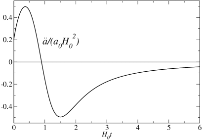
Figure 1: The exit of inflation and the beginning of deceleration.

Let us now lay radiation aside and allow the photons to gain mass. In that purpose, we will choose the potential $V(\Phi^{2})=\mu e^{-\lambda\Phi^{2}}$, where $\mu$ and $\lambda$ are constants. It is clear that, as $\Phi$ rolls down the potential hill towards non-zero values, the photons acquire an effective mass. Therefore this choice of potential can describe a scalar field that decays to massive vector bosons, which, in turn, can be responsible for dark matter in the Universe. To carry that out, we have to abandon our previous interpretation of the energy density of the fields which distinguish between $\rho_{\cal J}$ and $\rho_{\rm r}$, and ascribe to the massive vector field the energy density $\rho_{\rm dm}=\rho_{\rm r}+\rho_{\cal J}$ and pressure $p_{\rm dm}=p_{\rm r}+p_{\cal J}$, where the subscript alludes to dark matter. In this redefinition, $\rho_{\rm r}$ accounts for the kinetic part of the energy of the massive photons, while $\rho_{\cal J}$ owes to the contribution of its mass.

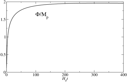
Figure 2: The growth of the scalar field.

By numerical analysis we extract the general features of the model. In figures 1 to 3 we plot the relevant intervals for $\ddot{a}(t)$, $\Phi(t)$ and the energy densities of the fields for a particular choice of parameters:

$$k=2a_{0}H_{0},\qquad q^{2}=0.05H_{0}^{2}M_{p}^{-2},\qquad\lambda=10M_{p}^{-2},\qquad\mu=0.7\rho_{0},$$

and initial conditions:

$$\cases{a(0)=a_{0},\qquad\dot{a}(0)=a_{0}H_{0},\qquad V(0)=0.6\rho_{0},\cr\dot{\Phi}(0)=0,\qquad\rho_{\rm r}(0)=k^{2}A_{i}A_{i}(0)/a_{0}^{4},\qquad\partial_{0}(A_{i}A_{i})(0)=0,}$$

where $M_{p}$ is defined by $M_{p}\equiv\sqrt{3/(8\pi G)}$ and $\rho_{0}=H_{0}^{2}M_{p}^{2}$. However, the behavior displayed is quite general and can be modeled by an adjustment of the parameters and initial conditions. It is described as follows: during inflation the scalar field is next to $\Phi=0$, where the potential $V(\Phi^{2})$ is nearly flat and attains its maximal value. When the scalar field begins to depart from $\Phi=0$ and roll down the potential, inflation ends and the scalar field decays to massive vector bosons. The decay process is not abrupt; rather, there is a smooth transition from a domination of the scalar field to a domination of matter. Numerical solutions show that when the decay rate $2q^{2}A_{i}A^{i}\Phi\dot{\Phi}$ of the inflaton (see eq. (14)) ceases to be significant, the scalar field attains a roughly constant value, $\Phi_{\rm c}$, implying an effective mass of the vector bosons $m_{\rm dm}=\sqrt{2}q\Phi_{\rm c}$ (see eq. (11)), which, by this time, behave as ordinary matter with $p_{\rm dm}\approx 0$ and $\rho_{\rm dm}$ scaling as $\propto 1/a^{3}$, whereas $\rho_{\Phi}$ decays faster than $\propto 1/a^{4}$.

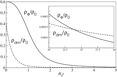
Figure 3: The behavior of the energy densities of the dark matter (dashed line) and of the scalar field (straight line) and the smooth transition from the domination of the scalar field to the domination of the massive vector field.

5.2 Quintessence

By taking another look at the equation of motion for the scalar field:

$$\ddot{\Phi}+3H\dot{\Phi}+{1\over 2}V^{\prime}=-{q^{2}\over a^{2}}A_{i}A_{i}\Phi$$

we can spot a new term at the right hand side of the equality which is absent in the case of a non-interacting scalar field. This term shows up due to the interaction with the vector field, and it resembles an elastic force ($F=-kx$) whose time-dependent “elastic constant” is $q^{2}A_{i}A_{i}/a^{2}$. This force acts on the motion of the scalar field by drawing it towards the position $\Phi=0$. When the scalar field is subject to a potential $V(\Phi^{2})$ whose minimum lies at $\Phi=0$ the influence of this force will not alter significantly the qualitative behavior of the scalar field, but, on the contrary, if $\Phi=0$ is not a minimum, there must arise relevant modifications in its motion.

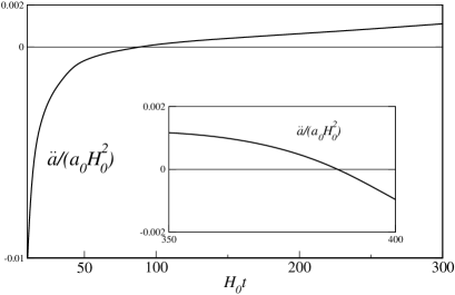
Figure 4: Accelerated expansion driven by the quintessence field. In the small frame: end of quintessence era.

That is what we shall investigate in this section by considering the “Mexican Hat” potential

$$V(\Phi^{2})=\lambda(\Phi^{2}-\Phi^{2}_{0})^{2},\qquad\hbox{where}\qquad\Phi^{2}=\Phi^{2}_{0}$$

corresponds to the lowest state. It is clear that the vacuum solution $\Phi^{2}=\Phi^{2}_{0}$ and $A_{\mu}=0$ satisfies eqs. (10) and (11).

However, in the presence of vector bosons (i.e., if $A_{i}A_{i}\not=0$), the ground state for the scalar field becomes an unstable position, for if we place $\Phi$ at $\Phi_{0}$, it will be pulled toward the origin due to the term $-q^{2}A_{i}A_{i}\Phi/a^{2}$.

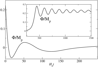
Figure 5: The behavior of the field $\Phi$: (i) during the quintessence era; (ii) in the subsequent period when it rolls back to its potential minimum and oscillates about it (small frame).

With the following choice of parameters:

$$k^{2}=0.7a_{0}^{2}H_{0}^{2},\quad q^{2}=0.5H_{0}^{2}M_{p}^{-2},\quad\lambda=0.01H_{0}^{2}M_{p}^{-2},\quad\Phi_{0}^{2}=0.05M_{p}^{2},$$

we have solved numerically the system (30), (31) and (32) with initial conditions

$$\cases{a(0)=a_{0},\qquad\dot{a}(0)=a_{0}H_{0},\qquad\Phi(0)=\Phi_{0},\cr\dot{\Phi}(0)=0,\qquad\rho_{\rm r}(0)=k^{2}A_{i}A_{i}(0)/a_{0}^{4},\quad\partial_{0}(A_{i}A_{i})(0)=0,}$$

that corresponds to placing $\Phi$ in its ground state ($\rho_{\Phi}=0$) and filling the Universe with radiation. In figures 4 to 6 we plot the relevant intervals for $\ddot{a}(t)$, $\Phi(t)$ and the energy densities of the fields.

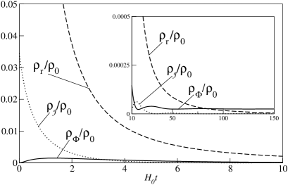
Figure 6: The coupling to radiation transfers energy to the field $\Phi$, which later comes to dominate and behaves as quintessence (small frame). Energy densities: scalar field – straight line; current field – dotted line; radiation field – dashed line.

The coupling of the scalar field to radiation removes it from its ground state and makes it climb up the potential hill to positions near the origin. That raises its potential energy and confers on it a quintessential behavior. During the period that $\Phi$ remains next to $\Phi=0$ the acceleration becomes positive, $\rho_{\rm r}$ goes as $\propto 1/a^{4}$ and the vector bosons can be, meanwhile, regarded as radiation. This period can be made as long as one wishes by a suitable choice of the parameters. But, ultimately, the force that keeps $\Phi$ next to zero becomes too weak and $\Phi$ rolls back to (one of) its ground state(s), oscillating about it. Consequently, the symmetry is spontaneously broken, the photons become massive , and the expansion decelerates again.

As a final remark we note that, in this model, the positive acceleration of the Universe is not due to a small non-zero vacuum energy [14, 22, 5]. Here, the vacuum energy is indeed zero, but the point is that the Universe is not in the vacuum state. It is filled with particles that, due to their interactions, displace the fields from their ground states and make them act as dark energy. Motivated by this we suggest that a possible explanation for the present acceleration of the Universe might reside in the fact that the Universe is (obviously) not in vacuum although its energy density is very small, and the interactions among its constituents, which so far have been commonly neglected, might be responsible for the dark energy.

6 Conclusions and Outlook

To sum up, we remark that the qualitative treatment performed here point out to interesting mechanisms of accounting for the dark-matter in the Universe (or at least a part of it), and also provides a possible candidate for quintessence. However, the quintessence behavior displayed here differs from the usual quintessence models in the sense that the scalar field is not tending asymptotically to the minimum of its potential. Rather, its minimum is not a stable position and the scalar field is removed from its ground state due to its coupling to a background field of vector bosons.

All the same, our study is not complete and a quantitative confrontation of the predictions yield by these models to observations is needful. Besides taking into account the full spectrum, it is also necessary to address the issue of whether the models treated here satisfy the constraints from the anisotropy of the CMBR, the large-scale galaxy distribution and the SN-Ia data. That will be performed in a future work.

References

References

- [1] Ratra B and Peebles P J E 1988 Phys. Rev. D 37 3406 Guth A H 1981 Phys. Rev. D 23 347 Olive K A 1990 Phys. Rep. 190 307
- [2] Kremer G M and Devecchi F P 2002 Phys. Rev. D 66 063503 Kremer G M and Devecchi F P 2003 Phys. Rev. D 67 047301 Kremer G M 2003 Gen. Relat. Grav. 35 1459 Kremer G M 2003 Phys. Rev. D 68 123507 Kremer G M and Alves D S M 2004 Gen.Rel.Grav. 36 2039
- [3] Linde A 1990 Particle Physics and Inflationary Cosmology (Chur: Harwood Academic Publishers)
- [4] Kolb E W and Turner M S 1990 The Early Universe (Boulder: Westview Press)
- [5] Peebles P J E and Ratra B 2003 Rev. Mod. Phys. 75 559 Padmanabhan T 2003 Phys. Rept. 380 235
- [6] Wetterich C 1988 Nucl. Phys. B 302 668 Ratra B Peebles P J 1988 Phys. Rev. D 37 3406 Frieman J A, Hill C T, Stebbins A and Waga I 1995 Phys. Rev. Lett. 75 2077 Caldwell R R, Dave R and Steinhardt P J 1998 Phys. Rev. Lett. 80 1582 Zlatev I, Wang L and Steinhardt P J 1999 Phys. Rev. Lett 82 896 Uzan J P 1999 Phys. Rev. D 59 123510 Chiba T 1999 Phys. Rev. D 60 083508 Amendola L 1999 Phys. Rev. D 60 043501
- [7] Linde A D 1982 Phys. Lett. 108B 389 Abbot L F, Fahri E and Wise M 1982 Phys. Lett. 117B 29 Dolgov A D and Linde A D 1982 Phys. Lett. 116B 329 Lyth D H and Riotto A 1999 Phys. Rept. 314 1
- [8] Albrecht A, Steinhardt P J, Turner M S and Wilczek F 1982 Phys. Rev. Lett. 48 1437
- [9] Dolgov A D and Kirilova D P 1990 Sov. J. Nucl. Phys. 51 172 Traschen J H and Brandenberger R H 1990 Phys. Rev. D 42 2491
- [10] Kofman L, Linde A and Starobinsky A A 1997 Phys. Rev. D 56 3258
- [11] Kofman L, Linde A and Starobinsky A A 1994 Phys. Rev. Lett. 73 3195
- [12] Perlmutter S et al1999 Astrophys. J. 517 565 Riess A G et al2001 Astrophys. J. 560 49 Turner M S and Riess A G 2002 Astrophys. J. 569 18 Tonry J et al2003 Astrophys. J. 594 1
- [13] Bennett C L et al2003 Astrophys. J. Suppl. 148 1 Peiris H V et al2003 Astrophys. J. Suppl. 148 213 Netterfield C et al2002 Astrophys. J. 571 604 Halverson N et al2002 Astrophys. J. 568 38 Spergel D N et al2003 Astrophys. J. Suppl. 148 175 Riess A G et al1998 Astrophys. J. 116 1009
- [14] Carroll S M 2003 Preprint astro-ph/0310342
- [15] Schmidt B et al1998 Astrophys. J. 507 46 Turner M S and Riess A G 2002 Astrophys. J. 569 18 Efstathiou G et al1998 Preperint astro- ph/9812226 Huterer D and Turner M S 1999 Phys. Rev. D 60 081301
- [16] Nesteruk A V 1999 Gen. Rel. Grav. 31 983 Zimdahl W, Balakin A, Schwarz D and Pavón D 2002 Grav. Cosmol. 8 158 Billyard A P and Coley A A 2000 Phys. Rev. D 61 083503 Berera A 1995 Phys. Rev. Lett. 75 3218 Wetterich C 1995 Astron. Astrophys. 301 321 de Oliveira H P and Ramos R O 1998 Phys. Rev. D 57 741 Cardone V F, Troisi A and Capozziello S 2004 Phys. Rev. D 69 083517 Copeland E J, Nunes N J and Pospelov M 2004 Phys. Rev. D 69 023501 Chimento L P, Jakubi A S, Pavón D and Zimdahl W 2003 Phys. Rev. D 67 083513 Amendola L 2000 Phys. Rev. D 62 043511
- [17] Bailin D & Love A 1993 Introduction to Gauge Field Theory (Philadelphia: IOP Publishing)
- [18] Landau L and Lifshitz E M 1989 The Classical Theory of Fields 4th ed (New York: Pergamon Press)
- [19] Tolman R 1987 Thermodynamics and Cosmology (New York: Dover Publications)
- [20] Tolman R and Ehrenfest P 1930 Phys. Rev. 36 1791
- [21] Novello M, Bergliaffa S E P and Salim J 2003 Preprint astro-ph/0312093
- [22] Carroll S M 2001 Liv. Rev. Rel. 4 1
- [23] Felder G, Kofman L, Linde A and Tkachev I 2000 J. High Energy Phys. JHEP08(2000)010