Towards characterization of exoplanetary atmospheres with the VLT Interferometer

Abstract

The direct observation of extrasolar planets and their spectra is coming into reach with the new generation of ground-based near-IR interferometers, like the Very Large Telescope Interferometer (VLTI). The high contrast between star and planet requires an excellent calibration of atmospheric distortions. Proposed techniques are the observation of color-differential or closure phases. The differential phase, however, is only in a first order approximation independent of atmospheric influences because of dispersion effects. This might prevent differential phase observations of extrasolar planets. The closure phase, on the other hand, is immune to atmospheric phase errors and is therefore a promising alternative. We have modeled the response of the closure phase instrument AMBER at the VLTI to realistic models of known extrasolar planetary systems taking into account their theoretical spectra as well as the geometry of the VLTI. We present a strategy to determine the geometry of the planetary system and the spectrum of the extrasolar planet from closure phase observations in a deterministic way without any a priori assumptions. We show that the nulls in the closure phase do only depend on the system geometry but not on the planetary or stellar spectra. Therefore, the geometry of the system can be determined by measuring the nulls in the closure phase and braking the remaining ambiguity due to the unknown system orientation by means of observations at different hour angles. Based on the known geometry, the planet spectrum can be directly synthesized from the closure phases.

1 Introduction

Since the first extrasolar planet candidate was discovered in 1995 orbiting the solar-like star 51 Peg (Mayor & Queloz 1995), more than 130 extrasolar planets have been detected by radial velocity surveys (e.g. Mayor et al. 2003 for recent discoveries). So far, the only observational information on the spectrum of an extrasolar planet has been obtained for the transiting system HD209458 (e.g. Charbonnneau et al. 2002, Vidal-Madjar et al. 2004).

Figure 1: Spectral signal of planet in the closure phase. Top panel: theoretical near-IR spectrum of the extrasolar planet orbiting 51 Peg displaying CO and H₂O absorption bands (Sudarsky, Burrows & Hubeny 2003). Bottom panel: closure phases in milliradian calculated by us based on the theoretical spectrum of 51 Peg b shown above as well as on the stellar spectrum for a simulated observation with the near-IR instrument AMBER/VLTI using the three telescopes UT1, UT3 and UT4 (baseline length 102m, 62m, 130m). It is evident that the spectrally resolved closure phases contain a wealth of spectral information of the planet.

In order to gain deeper insights into the physics of extrasolar planets and directly detect e.g. their atmospheres, observations with milliarcsec spatial resolution and at an unprecedented dynamical range are required (e.g. 10^-5 in the near-IR for 51 Peg). Such observations are coming into reach with the new generation of ground-based near-IR interferometers, like the VLTI. Observations of high contrast systems, like extrasolar planets, require an excellent calibration of atmospheric distortions. It has been proposed to observe extrasolar planets and their spectra through the differential phase or closure phase method (e.g. Quirrenbach & Mariotti 1997, Akeson & Swain 1999, Quirrenbach 2000, Lopez & Petrov 2000, Segransan 2001, Vannier et al. 2004). An overview of the mathematical basis for the observations of interferometric phases of extrasolar planets has also been provided by Meisner (2001) and in particular on the web page referenced therein.

Differential phases are measured between different wavelength bands, which, in a first order approximation, are subject to the same optical path length fluctuations introduced by atmospheric turbulence. The resulting differential phase errors can therefore be eliminated in the data reduction to a certain degree. However, higher order effects due to random dispersion in the atmosphere as well as in the delay lines (caused mainly by variations of the humidity of the air) can be a significant source of systematic errors and might prevent one from reaching the necessary precision to observe differential phases of extrasolar planets.

A more promising approach is the observation of closure phases, which are measured for a closed chain of three or more telescopes. The closure phase $\Phi_{\mathrm{cl}}$ is the sum of the individual single-baseline phases $\Phi_{ij}$ measured on the baseline between telescope $i$ and $j$ of the array:

$$\Phi_{\mathrm{cl}}=\Phi_{12}+\Phi_{23}+\Phi_{31}.$$

The closure phase is independent of atmospheric phase errors and allows therefore a self-calibration, which was first recognized by Jennison (1958).

Closure phase observations from the ground will be possible with the AMBER (Astronomical Multi-BEam combineR) instrument at the VLTI operated by ESO (Petrov et al. 2003, Malbet et al. 2004) . AMBER is operating in the near-IR J, H, and K bands from 1.1 to 2.4$\mu$m. It is currently undergoing commissioning at Cerro Paranal and is scheduled to be available for regular observations in 2005. With a multi-beam combiner element and a fringe dispersing mode, it has the capability of combining the light of three telescopes (UTs or ATs), and performing spectrally resolved differential and closure phase observations. There are three different spectral resolutions available: low (R=$\lambda$/$\Delta\lambda$=35), medium (R=500…1000) and high (R=10000…15000).

We have modeled the response of the AMBER instrument at the VLTI for known extrasolar planetary systems taking into account their theoretical spectra as well as the geometry of the VLTI. The closure phase depends not only on the contrast ratio between planet and star but also on the (generally unknown) system geometry as well as on the interferometer geometry and the hour angle of observation. In the following, we present a method to determine the planetary system geometry and the planet spectrum from closure phase observations in a deterministic way without any a priori assumptions.

Figure 2: Relation between the closure phase and the corresponding single-baseline phases. The figure shows simulated phase measurements for a system comprised of two point sources with a 3 milliarcsec separation and a constant flux ratio of the components of 10^-3 observed at zenith with the VLTI telescopes UT1, UT3 and UT4. The three top panels display the phases calculated for the single-baselines B₁₂, B₂₃ and B₃₁. (We note that they cannot be measured without a phase reference (e.g. PRIMA) and are displayed here only for theoretical considerations.) The bottom panel shows the simulated closure phase for these three telescopes. All phases are in millirad. It is evident that the nulls in the closure phase are always also nulls in the single-baselines phases. In particular, every second null of a single-baseline phase is also a null in the closure phase.

2 Modeling of closure phases of exoplanets

We have written a code to simulate closure phase observations with AMBER for known extrasolar planetary systems, taking into account their theoretical spectra as well as the geometry of the VLTI. We use theoretical spectra, which have been calculated by Sudarsky, Burrows & Hubeny 2003 (see their paper for details). For the separation between star and planet the published semi-major axis is taken, whereas the orientation of the system is unknown and an arbitrary value was chosen for the purpose of the simulations.

Fig.1 displays in the top panel a theoretical spectrum of the giant irradiated planet orbiting the solar-like star 51 Peg. The bottom panel of Fig. 1 shows the modeled closure phase response to the planetary system 51 Peg in a simulated observation with AMBER and the three 8 m unit telescopes UT1, UT3 and UT4 (baseline lengths 102m, 62m, 130m).

It can be seen from Fig.1 that the spectrally resolved closure phases contain information on the planetary spectrum. However, they also depend on the interferometer geometry, the hour angle of the observations, the spectra of the star, and on the planetary system geometry. The latter is generally unknown for radial velocity planets.

Further results of the simulations are shown in Fig.2 and Fig.3 and are discussed in the following sections.

3 Nulls in the closure phase

We show in this section that the nulls in the closure phase are independent of the planet / star contrast ratio but do only depend on the planetary system geometry, i.e. separation and orientation of the system. Therefore, the measurement of the wavelength for which the closure phase is zero, is the first step in disentangling the planet spectrum from the closure phase.

In a mathematical sense, the condition for single-baseline phases $\Phi_{ij}$ to be zero is that the dot product between separation vector $\vec{s}$ (pointing from the star to the planet) and the corresponding projected baseline $\vec{B_{ij}}$ equals multiples of $\lambda/2$:

$$\vec{s}*\vec{B_{ij}}=n\cdot\lambda/2\quad\Longrightarrow\quad\Phi_{ij}=0.$$ (1)

Thus, the nulls in the single-baseline phase depend only on the interferometer geometry $\vec{B_{ij}}$ and the planetary system geometry $\vec{s}$, but are independent of the planet and star spectra. (We note that the absolute interferometric phase measured on a single-baseline is not an accessible quantity without phase referencing, as planned for example for the instrument PRIMA, which is under development for the VLTI.)

We have shown analytically (Joergens & Quirrenbach 2004) that there is also a simple condition for nulls in the closure phase: the closure phase is zero if the dot product between separation vector $\vec{s}$ and one of the involved baseline vectors $\vec{B_{ij}}$ equals multiples of $\lambda$:

$$\vec{s}*\vec{B_{ij}}=n\cdot\lambda\quad\Longleftrightarrow\quad|s|\cdot|B_{ij}|~{}\vartheta_{ij}=n\cdot\lambda$$ (2)

$$\Longrightarrow\quad\Phi_{\mathrm{cl}}=\sum_{ij}\Phi_{ij}=0$$ (3)

with $\vartheta_{ij}$ being the angle between $\vec{s}$ and $\vec{B_{ij}}$.

Comparison with Eqn. 1 shows that for every second null in a single-baseline phase, the closure phase has also a null.

This is illustrated by Fig.2, which displays the simulated single-baseline as well as closure phases for two point sources with a constant contrast ratio of 10^-3 for all wavelengths. Considering such a ’flat spectrum’ allows us to show the relation between the closure phase and the corresponding individual phases without the complication of the complex spectral features of the source. It can be seen from the plot that the nulls in the closure phase are always also nulls in one of the corresponding single-baseline phases. Furthermore, every second null of a single-baseline phase is also a null in the closure phase.

This shows that the nulls in the closure phase are also independent of the planet / star contrast ratio and do only depend on the system geometry.

4 Earth rotational synthesis

We now proceed to describe an algorithm to determine the spectrum of a planet and the geometry of the star-planet system (i.e. the angular separation and position angle of the planet with respect to the star at the time of observation) from closure phase observations, without any a priori knowledge of these quantities. The stellar spectrum can be presumed to be known, however, since this is easily measurable with a simple spectrograph. Determining the planet spectrum is therefore equivalent to measuring the planet / star contrast ratio.

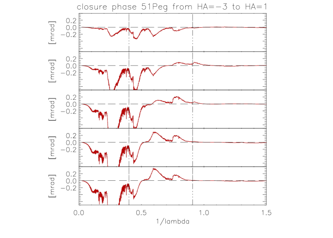
Figure 3: Closure phase time series for the planet system 51 Peg. Simulations for observations with the VLTI array UT1, UT3, UT4 for hour angles HA = -3, -2, -1, 0, +1 hr (from top to bottom). Vertical lines indicate the wavelength range covered by AMBER (the near-IR bands between 1.1 $\mu$m and 2.5 $\mu$m).

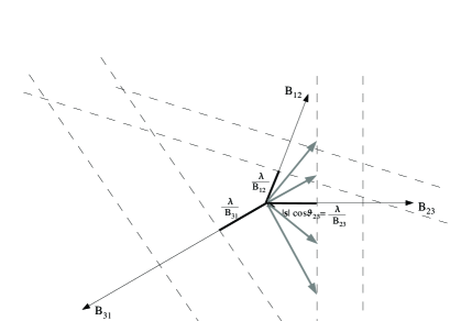
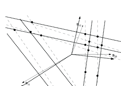
Figure 4: Possible geometries of a star – planet system as derived from nulls of the closure phase. Left: Determination of the nulls in the closure phase signal of a planetary system at a certain hour angle is a measure for the projection of the separation vector $\vec{s}$ between star and planet onto one of the three projected baselines. Due to the unknown orientation $\vartheta_{ij}$ we do not know onto which one. The dashed lines indicate the possible locations of $\vec{s}$ for the nulls corresponding to $n=1$ and 2. Right: Observations at a later hour angle gives another set of lines. The possible locations for $\vec{s}$ are now reduced to several grid points as marked by the intersections with the former lines. With a third observation, it will be possible to select the correct intersection point.

As described in the previous section, the nulls of the closure phase contain information about the system geometry because they are related to the nulls of the single-baseline phases. However, it is not known a priori to which single baselines the individual nulls in the closure phase correspond. We can thus interpret Eqn. 2 as follows: By determining a wavelength for which the closure phase is zero, we have a measure for the projection $|\vec{s}|\cdot\vartheta_{ij}$ of the separation vector $\vec{s}$ onto one of the individual baselines $\vec{B_{ij}}$ but we do not know onto which one. Furthermore, we do not necessarily know the order $n$ of the null. The geometrical locus of all possibilities for $\vec{s}$ is therefore a set of straight lines, as shown in the left panel of Fig. 4. Each line in this figure is perpendicular to one of the baselines and corresponds to an assumed set of $i,j,n$. For clarity only the lines corresponding to $n$ = 1 and $n$ = 2 are shown.

The set of projected baseline vectors formed by the three telescopes changes with time due to Earth’s rotation. Therefore, a second observation gives an independent constraint on the geometry as shown in the right panel of Fig. 4. The possible system geometries are now the intersections of the set of lines corresponding to the first observation with the set corresponding to the second. This discrete set of points has been marked with filled circles in the figure. A third observation will produce yet another independent set of lines. In general, this set will pass through only one of the previously marked points: this is the true separation vector. It is thus possible to derive the system geometry unambiguously with three observations.

Once the separation vector is known, it is straightforward to determine the planet / star contrast ratio for each wavelength through a numerical inversion of the expression for the closure phase. The only difficulty occurs at or very close to the nulls, where the signal-to-noise is zero or very low. However, since three observations are needed in any case for the determination of $\vec{s}$, one can perform the three inversions and combine them with (wavelength-dependent) weights appropriate for their respective signal-to-noise ratios. Consider, for example, the wavelength range around $\lambda=1.67\,\mu$m ($1/\lambda=0.6\,\mu$m^-1) in Fig. 3. The observation at $-1$ hr (third panel) gives very low signal-to-noise close to the null near $1/\lambda=0.6\,\mu$m^-1, but observations at other times can be used to infer the planet spectrum in this wavelength region.

5 Outlook

We have shown that the separation vector and spectrum of extrasolar planets can be determined from closure phase measurements in a deterministic way, with a non-iterative algorithm, and without any a priori assumptions. For a practical application of this technique, a few additional complications will have to be considered:

• The assumption that the star and the planet are point sources will have to be relaxed. Taking into account that the star is slightly resolved by the interferometer complicates the analysis and implies that the relation between nulls in the closure phase and the single-baseline phases is only approximately fulfilled.

• For observations from the ground, the useful wavelength range in the near-infrared is limited to the atmospheric windows and thus non-contiguous.

• The finite signal-to-noise ratio of realistic observations will lead to an uncertainty in determining the exact wavelengths of closure phase nulls. The lines and intersection points of Fig. 4 will thus be broadened.

• The non-zero time needed to accumulate sufficient signal-to-noise on the closure phase means that the interferometer geometry will change slightly during the observations. This is again equivalent to a slight broadening of the allowed regions in Fig. 4.

• If the time required to accumulate all observations is not short compared to the orbital period of the planet, the motion of the planet will also contribute an uncertainty in the derived geometry.

These practical complications will certainly be at least partially compensated by a larger number of observations; one would probably take ten or more rather than the minimum three. One could also combine the algorithm presented here with a global $\chi^{2}$ minimization, in which the orbital parameters and spectrum of the planet are fitted to the observations. The purpose of our algorithm would then consist of providing a robust starting point for the $\chi^{2}$ minimization algorithm, which is usually crucial to ensure convergence to the correct minimum.

The AMBER instrument has arrived on Cerro Paranal this year and the first commissioning runs have taken place. It is now necessary to determine if the required closure phase precision (better than 0.1 mrad, see Fig. 1) can be reached. If so, the VLTI will provide unprecedented opportunities for observations of extrasolar planets and their spectra.