Error analysis of quadratic power spectrum estimates for CMB polarization: sampling covariance
Abstract
Quadratic methods with heuristic weighting (e.g. pseudo- or correlation function methods) represent an efficient way to estimate power spectra of the cosmic microwave background (CMB) anisotropies and their polarization. We construct the sample covariance properties of such estimators for CMB polarization, and develop semi-analytic techniques to approximate the pseudo- sample covariance matrices at high Legendre multipoles, taking account of the geometric effects of mode coupling and the mixing between the electric () and magnetic () polarization that arise for observations covering only part of the sky. The - mixing ultimately limits the applicability of heuristically-weighted quadratic methods to searches for the gravitational-wave signal in the large-angle -mode polarization, even for methods that can recover (exactly) unbiased estimates of the -mode power. We show that for surveys covering one or two per cent of the sky, the contribution of -mode power to the covariance of the recovered -mode power spectrum typically limits the tensor-to-scalar ratio that can be probed with such methods to .
keywords:
cosmic microwave background – methods: analytical: – methods: numerical.1 Introduction
With the recent results from the Degree Angular Scale Interferometer (DASI; Kovac et al. 2002; Leitch et al. 2004), the Cosmic Anisotropy Mapper (CAPMAP; Barkats et al. 2005) and the Cosmic Background Imager (CBI; Readhead et al. 2004), and the imminent two-year results from the Wilkinson Microwave Anisotropy Probe (WMAP; Kogut et al. 2003), the characterization of the polarization of the cosmic microwave background (CMB) polarization is gathering pace. The ultimate goal of such experiments is to constrain parameters describing the cosmological model and its fluctuations, and hence test models for the generation of these fluctuations, such as inflation. In Gaussian theories, all of the cosmological information encoded in the CMB anisotropies and their polarization is contained in their power spectra. For this reason, estimating CMB power spectra is a useful and efficient form of data compression in analysis pipelines (Bond, Jaffe & Knox, Bond et al.2000). However, estimating the spectra is not enough: it is also essential to have an accurate covariance matrix, and preferably an accurate model for the shape of the likelihood function (see e.g. Bond et al.2000; Efstathiou 2004). Modelling the covariance matrix for a particularly efficient class of polarization power spectra estimators – heuristically-weighted quadratic estimators, or pseudo-s – is the subject of this paper.
The polarization field can be decomposed uniquely on the full sky into a gradient part, with electric () parity, and a curl part with magnetic () parity (Kamionkowski, Kosowsky & Stebbins, Kamionkowski et al.1997; Seljak & Zaldarriaga, 1997). The cosmological importance of this decomposition is that linear density perturbations cannot produce magnetic polarization, and so, in standard scenarios and at linear order, large-angle -mode polarization is produced solely by gravitational waves. Second-order effects, most notably weak gravitational lensing by large-scale structure, can generate modes from primary modes (Zaldarriaga & Seljak, 1998). The lens-induced modes have a blue spectrum, and should dominate any primary signal from gravitational waves on sub-degree scales. On larger scales, they may still dominate if the gravitational wave amplitude is sufficiently low. Either way, the variance of the modes is expected to be much smaller than that of the modes. Given the different parity properties of the and fields, CMB polarization in a statistically-isotropic and parity-respecting universe is characterized by two power spectra, and , and also the cross-power between and the temperature anisotropies.
A number of different methods have been developed to estimate these CMB polarization power spectra. The optimal method, brute-force maximum likelihood (e.g. Górski 1994; Bond, Jaffe & Knox Bond et al.1998), and its quadratic approximation (Tegmark & de Oliveira-Costa, 2002), should produce the most accurate (minimum-variance) estimates. However, these methods require the inversion of matrices, where is the number of pixels in the map, which is prohibitively slow for the analysis of mega-pixel maps. Given these limitations, a number of fast alternative methods have been suggested (Hansen & Górski, 2003; Kogut et al., 2003; Chon et al., 2004) building on earlier work on the analysis of the temperature anisotropies (Szapudi, Prunet & Colombi, Szapudi et al.2001, Wandelt et al.2001; Hivon et al., 2002; Hansen, Górski & Hivon, Hansen et al.2002). These fast methods are closely related, and all involve compressing heuristically-weighted maps of the Stokes parameters into a set of pseudo-s making use of spherical transforms – a step that requires only operations with fast Fourier transform methods on iso-latitude pixelisations such as the widely-used HEALPix (Górski et al., 2004). The methods differ in the details of how they transform the pseudo-s to power spectrum estimates. In the absence of instrument noise, the mean of the pseudo-s is linear in the true power spectra, so, for observations over a large enough part of the sky, unbiased power spectrum estimates can be obtained by applying the inverse operation to the pseudo-s (Kogut et al., 2003). If the observed part of the sky is sufficiently small, direct inversion is not possible and some form of regularisation is required. Hansen & Górski (2003) advocate using likelihood methods, while Chon et al. (2004) make use of correlation functions as an intermediate data product. A notable feature of the latter approach is that the inversion is constructed so that electric and magnetic polarization power is not mixed in the mean. Pseudo- methods have now been applied to a number of real data sets, both for temperature (Netterfield et al., 2002; Hinshaw et al., 2003) and polarization analyses (Kogut et al., 2003; Ponthieu et al., 2005).
Despite the attention that pseudo- techniques have received, relatively little work has been done on trying to understand their error properties. This paper aims to fill that gap by providing the basis for a reliable, semi-analytic error analysis technique for CMB polarization power spectrum estimates obtained with pseudo- methods. This extends earlier analytic work that discusses temperature anisotropies only (Hinshaw et al., 2003; Efstathiou, 2004), and the recent thesis work by one of us (Chon, 2003) where both temperature and polarization are considered. A significant complication that arises for polarized data is the mixing of and modes for observations covering only part of the sky (Lewis, Challinor & Turok, Lewis et al.2002; Bunn et al., 2003). We develop approximations to the pseudo- sample covariances, taking this mixing into account at leading order for maps with smoothly-apodized edges. Our approximations are accurate in the regime where the mixing is perturbative, i.e. for , where is the effective band-limit of the function used to weight the Stokes parameters. It is difficult to construct good approximations for the covariance on large scales, . This is partly because of the increased importance of - mixing there, but also because the polarization power spectra do not go smoothly to zero on large scales in the presence of reionization. (The behaviour of the temperature-anisotropy power spectrum on large scales produces a similar effect for the temperature pseudo- covariance.) Following Efstathiou (2004), the low- sector of the covariance matrices can be constructed directly with exact methods, and used to overwrite the inaccurate approximation. Being able to evaluate accurate covariances efficiently is important in any application where multiple evaluations are required. Examples include parameter estimation, where the covariance generally depends on position in parameter space, and optimising the design and analysis of surveys, where one might wish to assess a large number of weighting schemes.
Throughout, we ignore the effects of instrument noise so we deal only with the sample covariance of the . This is to highlight the geometric effects of heuristic weighting that are peculiar to polarization analysis, particularly - mixing. An obvious extension of this work that will be required for application to real data is to include the contribution from instrument noise. For uncorrelated noise this should be straightforward, but in a more realistic set-up, one will probably have to resort to Monte-Carlo simulations for the noise contribution.
As noted above, one of the future goals of CMB polarization observations is to detect (or constrain) the stochastic gravitational wave background via its signature in large-angle -mode polarization (Seljak & Zaldarriaga, 1997; , Kamionkowski et al.1997). Magnetic polarization allows much smaller amplitude gravitational wave backgrounds to be detected than with temperature or electric polarization alone, since, in the latter case, the gravitational-wave signal is swamped by the cosmic variance of the signal from the dominant density perturbations. Methods to separate out exactly pure magnetic modes from observations with incomplete sky coverage exist at the map level (, Lewis et al.2002; Bunn et al., 2003; Lewis, 2003). Such methods have the desirable property that quadratic power spectrum estimates formed from the pure- modes have no cosmic variance if the -mode power is zero. Were it not for gravitational lensing, separating modes at the level of the map would thus allow the detection of arbitrarily low amplitude gravitational wave backgrounds in the absence of instrument noise. In practice, imperfections in removing the lensing signal limit the amplitude to tensor-to-scalar ratios111Our definition of the tensor-to-scalar ratio follows Martin & Schwarz (2000), i.e. it is the ratio of the primordial gravitational wave and curvature power spectra. (Kesden, Cooray & Kamionkowski Kesden et al.2002; Knox & Song 2002; see Seljak & Hirata 2004 for refinements from more optimal lensing-reconstruction methods). Heuristically-weighted pseudo- methods do not share the property that the cosmic variance of the estimated is immune to -mode power, even if we take care to construct unbiased estimates so that e.g. the mean of our estimator decouples from (Chon et al., 2004). We investigate this issue further here, exploring the limits of detectability for that arise solely from cosmic variance of the -mode polarization leaking into the variance of quadratic estimates of .
This paper is organised as follows. Section 2 reviews the properties of the polarization pseudo-s and establishes our notation. Following a brief discussion of the exact pseudo- covariance matrices in Section 3, we develop analytic approximations to them that can be rapidly computed in Section 4. We begin with a toy model, based on a Gaussian weight function applied to a small survey area in the flat-sky limit. (Some of the more involved manipulations are relegated to Appendix A.) This instructive example illustrates the key issues that are specific to the analysis of polarization, i.e. the geometric mixing of and modes. We then move on to develop approximations for arbitrary (smooth) weight functions, and test these against the exact covariances in cases where we can easily compute the latter (in particular, for azimuthally-symmetric weight functions). Simple rules-of-thumb for band-power variances are also derived in Section 4.4 as limiting cases of the more general expressions; some of the manipulations of the symbols required for these derivations are relegated to Appendix B. Finally, in Section 5 we consider the implications of our results for the detection of gravitational waves with -mode polarization estimated with pseudo- methods.
Throughout, we illustrate our results with the best-fitting power-law concordance CDM model to the Wilkinson Microwave Anisotropy Probe (WMAP) and 2dF Galaxy Redshift Survey data (Spergel et al. 2003; Table 7), but with the tensor-to-scalar ratio corresponding to inflation. We include the effects of gravitational lensing in the -mode power spectrum, but ignore effects due to its non-Gaussianity. Theoretical power spectra, pseudo-s and estimated power spectra in all figures include the smoothing effect of a Gaussian beam of ten-arcmin FWHM.
2 Properties of polarization pseudo-s
We define Stokes parameters along the line of sight using the basis vectors of a spherical polar coordinate system. We take the local axis to be and the axis ; these form a right-handed triad with the radiation propagation direction which defines the local axis. The complex polarization is then spin -2 (Newman & Penrose, 1966) and can properly be expanded in terms of spin-2 spherical harmonics (see e.g. Lewis et al.2002 for a review):
| (1) |
Reality of the Stokes parameters ensures that and similarly for , while under parity transformations (electric parity) but (magnetic parity). The polarization power spectra are defined in statistically-isotropic and parity-respecting models by
| (2) |
The - power vanishes (and is uncorrelated with the temperature anisotropies) by parity.
In pseudo- methods, one adopts a heuristic weighting of the complex polarization with a scalar function . The weight is necessarily zero in those regions that are not observed, but typically it is desirable to excise a larger region to remove further regions of high foreground emission. One can attempt to choose to improve the accuracy of subsequent power spectrum estimates. For example, on small scales, where the instrument noise dominates the signal, the optimal weighting is essentially inverse-noise-variance weighting (Efstathiou, 2004), while on large scales uniform weighting is preferable. In this paper we shall assume that the weight is chosen to be real and to go smoothly to zero as excised regions are approached. The former restriction ensures that the weighting does not alter the polarization direction, while the latter makes approximately band-limited to some . Such edge apodization allows us to deal with the effects of the resulting - mixing in the pseudo- covariance matrices in a perturbative manner; see Section 4. The problem of - mixing without edge apodization, i.e. taking everywhere one or zero, is discussed extensively by (Lewis et al.2002) and Lewis (2003) in the context of isolating modes at the map level.
Following Hansen & Górski (2003), we define pseudo-multipoles and to be the and -mode multipoles of the weighted polarization map, so that
| (3) |
where are the Hermitian coupling matrices
| (4) |
Using , and the reality of , we have which ensures that and a similar result for . If we expand the weight function in terms of its spherical multipoles, , the coupling matrices can be evaluated in terms of Wigner- symbols:
| (5) |
From equation (3) we can separate the and pseudo-multipoles as
| (6) | |||||
| (7) |
where we define the Hermitian to be
| (8) |
Given the and , we form their pseudo-s according to
| (9) |
We could also form , but, as we show shortly, this vanishes in the mean in the absence of parity violations. However, it may provide a useful test on parity-violating physics or unaccounted-for systematics, and so future data should, of course, be validated with .
In the absence of instrument noise, the mean pseudo-s (i.e. averaged over CMB realisations) are related to the true power spectra by convolutions. We find (Hansen & Górski, 2003)
| (10) |
where
| (13) | |||||
| (16) |
Here and we have introduced the power spectrum of the weight function . A non-zero matrix biases the pseudo-s by mixing e.g. -mode power into . For observations with uniform weight over the full sky, and since then only is non-zero and the symbol forces and hence to be even. The sum of and is approximately equal to the matrix that relates the temperature s to the mean pseudo-s (Hivon et al., 2002) at high . Their sum differs from the temperature case only by the presence of non-zero azimuthal quantum numbers in the symbol. The mean of evaluates to
| (17) |
and so vanishes if parity is preserved in the mean ().

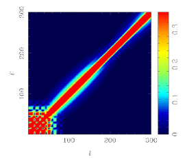
An example of the mean pseudo-s for observations over a circular region of radius is shown in Fig. 1. The weight function is uniform inside a circle of radius , but the remaining is apodized as so that falls smoothly to zero at the edge of the observed region. For this weight function the matrix is roughly two orders of magnitude larger than , and both are narrow compared to features in and except for the reionization signal on the largest scales. On small scales the mean pseudo-s can be approximated by removing and from the convolutions in equation (10) to give
| (18) |
For the mixing term described by is essentially negligible, and the mean of is approximately a scaled version of the underlying power spectrum. The relevant scaling is discussed below. For mixing is important, despite dominating over , since . This additional contribution to from geometric mixing of and modes can be clearly seen in Fig. 1, and, as expected, looks like a scaled version of the -mode power spectrum.
The normalisations and evaluate to
| (19) | |||||
| (20) |
where is defined by , and is the fraction of sky with non-zero weighting. Equation (19) follows from the expansions of and in equations (13) and (16), and the orthogonality of the symbols. It is the same normalisation as for the temperature anisotropies. Equation (20) can be established following the method used to derive equation (66) in Chon et al. (2004); see also Appendix B. Note that for much greater than the assumed band-limit of , the normalisation is suppressed by a factor compared to . This is consistent with the expectation that - mixing is suppressed at high (, Lewis et al.2002; Bunn et al., 2003). We can gain further insight into this result by noting that [for smooth ]
| (21) | |||||
| (22) |
where is smoothed with a top-hat (-space) filter. For band-limited weight functions, at the smoothing has little effect and so to leading order
| (23) |
At a given scale , the relative importance of mixing of - and -mode power in the pseudo-s is thus controlled by times the ratio of the average squared gradient of the weight function to the average square weight function.
2.1 Inversion of the pseudo-s
For the purpose of parameter estimation, it is not strictly necessary to attempt to invert the pseudo-s to (unbiased) power spectrum estimates. Forming the pseudo-s can be regarded as a mildly-lossy form of data compression of the maps of Stokes parameters, and inferences about cosmological models can be made directly from them if their covariance – or, better, their full sampling distribution – can be calculated (, Wandelt et al.2001). The calculation of the signal contribution to these covariances is the main topic of this paper. However, for presentation purposes it is useful to be able to plot quantities that are simply related to the underlying power spectra. At the least this requires some approximate deconvolution of the geometric effects of the weight function from the pseudo-s.
For observations covering enough of the sky222The criterion for invertibility is equivalent to being able to estimate the correlation functions for all angular separations (Chon et al., 2004). A sufficient condition is thus that the observed region has pixels separated by all angles between 0 and ., the matrices and will be invertible. In this case we easily obtain unbiased estimates of and from
| (24) |
Alternatively, we can form unbiased estimates of the correlation functions of the Stokes parameters from the polarization pseudo-s (or directly from the maps), and then invert these with the appropriate Legendre transforms (Chon et al., 2004). For observations over smaller parts of the sky, and will not be invertible. In this case we do not have the spectral resolution to obtain unbiased estimates of the s at every . Various approaches have been suggested to regularise the inversion including the use of band-powers (Hivon et al., 2002; , Hansen et al.2002), or apodized Legendre transforms of the (incomplete) correlation functions (, Szapudi et al.2001; Chon et al., 2004). The latter method provides estimates of the s convolved with a window function that depends only on the choice of apodizing function that is applied to the correlation function. Chon et al. (2004), building on earlier work by Crittenden et al. (2002), showed how to generalise the correlation function method to ensure that the estimated polarization power spectra did not mix and power in the mean. This is particularly useful for visualisation of the -mode power spectrum which can easily be swamped by the dominant modes. We do not reproduce the method of Chon et al. (2004) here, but note only that it provides a convenient way of constructing pseudo-inverses and to and respectively with the properties that
| (25) |
These relations ensure that our estimates of the power spectra,
| (26) |
satisfy and the equivalent relation for . The normalised window function , where is given by (Chon et al., 2004)
| (27) |
Here, are the reduced Wigner rotation matrices and is the apodizing function that is applied to the correlation functions. An example of the pseudo-inverses obtained via this route is shown in Fig. 1, along with the mean of the recovered s. The correlation functions have been apodized with a Gaussian with HWHM of . The apodizing function was deliberately chosen to be narrow to ensure that the resulting pseudo-inverses and are well localised. Given that the pseudo-inverses are significantly broader than and , the window function (not shown in the figure) inherits the width of the pseudo-inverses. For this reason the spectral resolution of the recovered s is rather poor compared to what should ultimately be achievable for a -radius survey. The effect of this is that the recovered s accurately follow the true s only for .
3 Exact covariance properties
The covariance of any quadratic power spectrum estimates that derive from the pseudo-s by linear transformations follow simply from the covariance of the latter. For this reason, in this paper we concentrate on the pseudo- covariance. Furthermore, we focus on the sample covariance (i.e. we neglect instrument noise) to highlight those aspects specific to CMB polarization that arise from mode-mixing on the incomplete sky. Including instrument noise is obviously important for application to near-future surveys since it will dominate sample variance. Extending the analytic results derived in this paper to include simple white noise should be straightforward (see Efstathiou 2004 for the case of the temperature anisotropies). However, for more realistic correlated noise, Monte-Carlo simulations will probably be required to account properly for the noise contribution to the covariances. We shall assume throughout that the CMB signal is Gaussian. If the initial fluctuations were very-nearly Gaussian, as expected in simple single-field inflation models (e.g. Bartolo et al. 2004), non-linear effects will introduce only a small level of non-Gaussianity into modes on the scales of interest for primary CMB science (e.g. Mollerach, Harari & Matarrese Mollerach et al.2004). However, if the primordial tensor-to-scalar ratio , then the dominant power in modes is expected to come from gravitational-lensing conversion of Gaussian modes into non-Gaussian modes. In this limit, our assumption of Gaussianity will be violated and the expressions derived in this paper will require some modification to account for the non-zero connected four-point function. While a full treatment of the pseudo- covariance in the presence of lens-induced modes is beyond the scope of the current paper, we note that the lensing contribution to has been calculated recently for uniform weighting in the flat-sky limit (Smith, Hu & Kaplinghat, Smith et al.2004).
In this section we calculate the exact sample covariance of and (see also Hansen & Górski 2003 for a similar calculation) and present the results of numerical computations for two types of survey: a full-sky survey with a simple Galactic cut, and a -radius circular survey of the type that is optimal for gravitational wave searches in the presence of instrument noise at the level achievable with current technology (Jaffe, Kamionkowski & Wang, 2000; , Lewis et al.2002).
For Gaussian CMB fields, the pseudo-multipoles are also Gaussian, so the covariance of their power spectra are given by e.g.
| (28) |
If we expand the pseudo-multipoles in terms of the true multipoles using equation (3), we find
| (29) | |||||
| (30) | |||||
| (31) |
Evaluating these expressions numerically is straightforward in principle, but is computationally expensive, with an operation count of if multipoles up to are retained. This is prohibitive for above a few hundred, and so, in general, there is a need for faster approximate calculations. One such approximation is to compute the covariances from Monte-Carlo simulations; this has the benefit of allowing one easily to include a number of real-world effects that are more difficult to include in the analytic calculation. An alternative, which is developed here in Section 4, is to use analytic approximations (that can be calibrated with simulations if required). As we show later, it is difficult to find good analytic approximations at low because of the expected sharp rise in the polarization s there, and the increased importance of - mixing. A similar problem arises for the temperature anisotropies because the s do not go smoothly to zero as . Efstathiou (2004) suggests replacing the block of the approximate covariance matrices with small and with the exact expression, since the latter can be calculated quickly at small and . For diagonally-dominant matrices, this procedure returns an accurate covariance matrix; a similar procedure can be implemented for polarization using equations (29)–(31) and the approximations developed in Section 4.
3.1 Examples
As our first application of equations (29)–(31), we consider a full-sky survey from which we remove a band around the Galactic plane. We adopt a north-south symmetric weighting which is uniform (which we expect to be nearly optimal in the noise-free limit) except for the edge of the retained survey which we apodize with the square of a cosine. In the northern hemisphere
| (32) |
Since is azimuthally-symmetric, the matrices are block diagonal and the covariances can be evaluated exactly in operations.
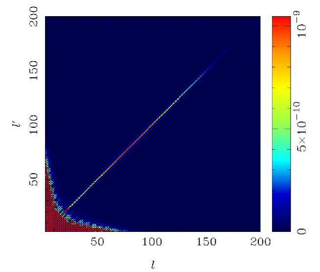
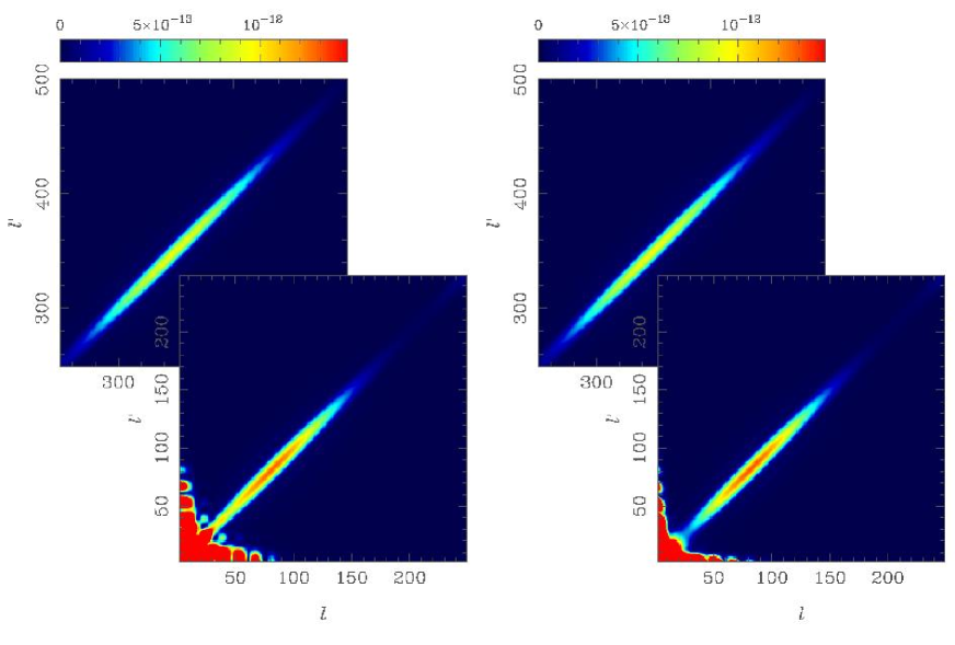
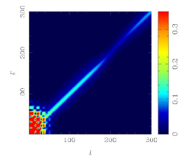
Figures 2–4 show the exact covariance matrices , and respectively. The prefactors have been chosen to make the elements near the diagonal more nearly uniform. Given that the weight function is symmetric under parity, and , so that and vanish if is odd, while vanishes if is even (and hence on the diagonal). In each of the three covariance matrices, the intense feature for and (which saturates the colour scale) arises predominantly from the additional power in on large scales due to reionization. (It vanishes if we substitute for power spectra with no reionization.)
In the case of , the first term inside the summation over and in equation (29) is always dominant. The covariance is thus very similar to that for the temperature anisotropies with the same weight function. The matrix is diagonally dominant, except on large scales, with width inversely related to the angular dimension of the retained region. On large scales the covariance matrix is dominated by the additional polarized power generated by reionization. Note that this power propagates to somewhat smaller scales in the pseudo- covariance due to residual Fourier ringing in the matrix . (For the weight function adopted here, the width of the main peak of is given by the inverse of the survey size, but the effective band-limit is larger being set by the inverse size of the apodized region.)
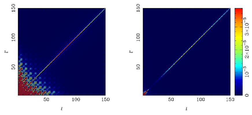
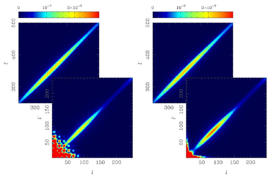
To emphasise the importance of - mixing in the structure of the covariance matrix for , in Fig. 3 we show both the exact and the matrix we obtain by setting . The latter is very inaccurate on the diagonal at , where - mixing is most important, and particularly so at the largest scales where it further fails to pick up the additional power in from reionization. Setting to zero also artificially suppresses the correlations: there is significantly more structure off the diagonal in the left-hand plot in Fig. 3 than on the right. This reflects the fact that is intrinsically broader than (see Fig. 1).
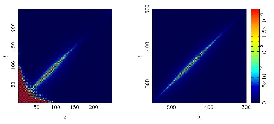
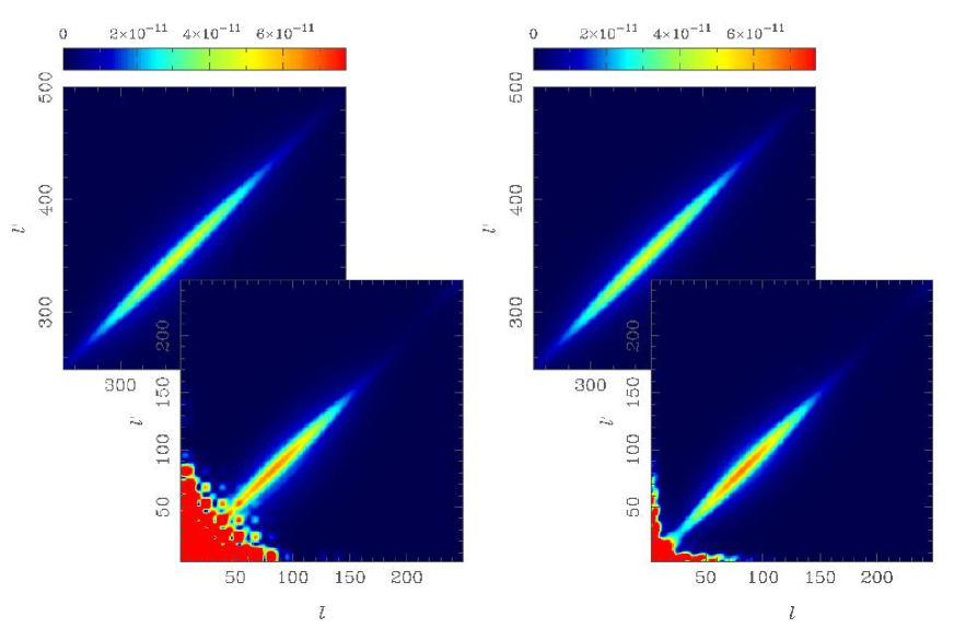
The covariance matrix , shown in Fig. 4, is only non-zero because of - mixing. It is correspondingly broader than . The dominant contribution is from -mode power, so the covariance matrix peaks near the diagonal at the positions of the acoustic peaks in .
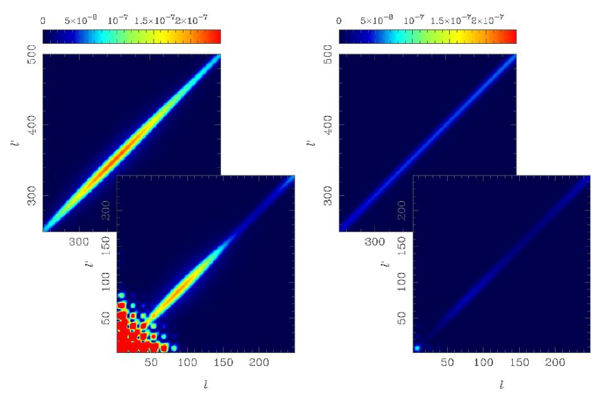
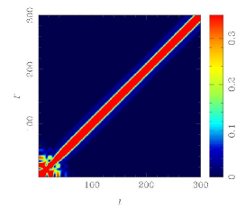
As our second example we consider the -radius survey with cosine apodization over the last that we used in Fig. 1. We should expect the relative importance of - mixing to extend to higher for this smaller survey, and this is indeed seen in Fig. 5 where we compare the exact with the covariance obtained by setting . The -mode power dominates the covariance for all scales plotted (maximum ), and the magnitude of the diagonal follows the acoustic peaks in . Surveys of this size are being considered by a number of upcoming experiments targeting -mode polarization from gravitational waves. It is clear that, even for the relatively optimistic tensor-to-scalar ratio adopted here (), the application of pseudo- techniques to such surveys will demand careful modelling of the impact of - mixing in the covariance matrix for on any scales where sample variance is expected to dominate.
4 Approximate covariances for smooth weighting
Given that exact evaluation of the pseudo- covariance matrices is, in general, prohibitively expensive, in this section we aim to derive accurate analytic approximations that allow fast computation of the covariances at high . This problem has been well-studied for temperature anisotropies (Hinshaw et al., 2003; Chon et al., 2004; Efstathiou, 2004), but, as yet, there has been no comparable treatment for polarization. As with the temperature case, the main simplification arises from assuming that we are working at sufficiently high , and with a weight function that is sufficiently band-limited, that we can approximate the s as being constant over the width of all coupling matrices. This removes the s from all convolutions. For , and its products, this approximation should be good, as in the temperature case, for smoothly-apodized observations covering a connected patch of linear extent more than several degrees. The approximation is poorer for , and breaks down completely if there is no apodization, i.e. the weight function is set to unity or zero. (See Lewis et al.2002 for examples of elements of in this case.) Here we restrict ourselves to situations where these assumptions hold. We first consider a specific case of Gaussian weighting over small patches of the sky, before considering general (but smooth) weighting on the sphere in Section 4.2.
4.1 Gaussian weighting in the flat-sky limit
As a warm-up to the approximate calculation of the pseudo- covariances for general weighting functions , we first consider Gaussian weighting over small patches of the sky. For such observations we can approximate the spherical-harmonic analysis by Fourier analysis, and we are able to make analytic progress more simply than for the general case. The results of this subsection are also of considerable interest for observations of CMB polarization with interferometers [such as DASI (Kovac et al., 2002), CBI (Readhead et al., 2004) and the Array for Microwave Background Anisotropy (AMiBA)333http://amiba.asiaa/sinica.edu.tw/], since they directly sample the Fourier transform of the sky multiplied by the primary beam. The latter thus acts as a weight function for an interferometer. Furthermore, the primary beam can often be approximated as a Gaussian.
In the flat-sky approximation, for lines of sight close to the axis, we adopt a global polarization basis that is aligned with the and axes. The radiation propagation direction at the centre of the field is along . Stokes parameters defined on this basis, and , at position on the sky can be decomposed into Fourier modes and :
| (33) |
From these we can define the Fourier transforms of the electric and magnetic parts of the polarization,
| (34) |
where is the angle between and the axis. Note that this is a rotation of the Stokes parameters in Fourier space onto a basis adapted to the wavevector . The Fourier transforms and can be shown to be related to the spherical multipoles and for by the same correspondence as for the temperature anisotropies, i.e.
| (35) |
A similar relation holds for . In terms of the power spectra, we have e.g. .
If the polarization is weighted by , then the Fourier transform of the Stokes parameters for the weighted field (or the visibilities in the case of an interferometer) are
| (36) | |||||
| (37) |
with a similar expression for . Here is the Fourier transform of . For real, and similarly for . Decomposing and as in equation (34), we find
| (38) |
or equivalently
| (39) | |||||
| (40) |
where the Hermitian [for real] kernels are
| (41) |
These are the flat-sky limits of the in equations (6) and (7). The geometric mixing of e.g. into is suppressed by the trigonometric factor . If the extent of the support of is [i.e. the band-limit of ] then the mixing of into the observable will be for . Clearly this is significant if .
4.1.1 Pseudo- covariance
In the flat-sky limit the pseudo-s are defined by
| (42) |
The signal correlations between the and are discussed in Appendix A. For Gaussian weighting, , and smooth spectra (over a range of multipoles ), we can use equations (150)–(152) to show that
| (43) |
where
| (44) | |||||
| (45) |
These results are consistent with equations (19) and (20), if we use and for , since the (spherical) power spectrum of the Gaussian weight function .
The sample covariances of the pseudo-s are given by the angular average of the squares of the correlators of and :
| (46) | |||||
| (47) | |||||
| (48) |
For an azimuthally-symmetric weight function, the correlators in these integrals are invariant under rigid rotations of and , so the integration over one of and is trivial. To evaluate equations (46)–(48) for the case of Gaussian weighting we make use of the results for the correlators given in Appendix A. The analysis is rather involved so we simplify things a little by considering only the limits and . If we consider the covariance of with itself, the case describes the contribution to the covariance if there were no - mixing, while the case describes the contribution that arises solely from mixing.
Consider first. Then, for azimuthally-symmetric , we have e.g.
| (49) |
where , and similar expressions hold for the other covariances. We have not been able to perform the integrals over exactly, but it is possible to make progress in the limit of large and (). In this limit, we can ignore the terms with factor in equations (152) and (155) in Appendix A. This leaves a factor of multiplying slowly-varying functions of . The exponential peaks sharply around (reflecting the fact that and are only strongly correlated for within a radius of ), so we can accurately handle the inverse powers of and trigonometric terms in equations (152) and (155) with an expansion in . To make this expansion it is useful to note that
| (50) | |||||
| (51) |
Integrating the square of the expansions over then yields a series of modified Bessel functions . These series are cumbersome, so we only give the leading-order results in the asymptotic regime (, ), where we can replace the Bessel functions with their asymptotic expansions:
| (52) | |||||
| (53) | |||||
| (54) |
To obtain these results it is necessary to expand the integrand in equation (49) to . It is straightforward to verify that the covariances of the pseudo-s for the other limit, , can be obtained by interchanging and in these expressions.
To gain an indication of how the covariance of the pseudo-s propagates to estimates of the power spectra, we form simple estimators for and that are local in and by solving equation (43):
| (55) |
where the normalisation . The covariance of these estimators then follows from the covariance of the pseudo-s which we derived above. To leading order, we find
| (56) |
and
| (57) |
Note that these expressions are symmetric in and as required. Equation (57), which gives the covariance of the estimated -mode power if there were no - mixing, is the direct analogue of the asymptotic expression for the temperature anisotropies, where the exact result in the flat-sky limit (for smooth ) is
| (58) |
If we average the estimators into bands of width we obtain quasi-uncorrelated estimates. The variances of these band-powers follows by integrating equations (56) and (57) over and within the band. For wide bands, we find the approximate results
| (59) | |||||
| (60) |
For the case, we recover the approximation given for temperature by Hivon et al. (2002),
| (61) |
noting that, for the case of Gaussian weighting considered here, and . In Section 4.4 we develop more general rules of thumb for arbitrary (but smooth) weight functions; these properly reduce to the expressions derived here for Gaussian weighting in the flat-sky limit.
Our leading-order results show that, for Gaussian weighting, the ratio of the cosmic variance contributions to from and is for . In Section 5 we consider the implications of this residual variance from -mode power in unbiased quadratic estimates of for detecting gravitational waves via -mode polarization.
4.2 Approximations for general weighting
We now consider the case of general (but smooth) weight functions and work on the spherical sky. The starting point is to approximate the correlators of the pseudo-multipoles that appear squared in the pseudo- covariances, equations (29)–(31), by removing the s from the convolutions:
| (62) | |||||
| (63) | |||||
| (64) | |||||
where are the matrices but evaluated with weight function rather than , and is the matrix product .444Due to the Hermiticity of , is also equal to . We now consider the derivation of equations (62)–(64) in detail. We start from the completeness relation which ensures that
| (65) | |||||
For or 0, so that , these relations imply that are projection operators (, Lewis et al.2002). If we express in terms of , using the obvious matrix notation, we find
| (66) |
Adding and subtracting gives
| (67) |
which can be used to verify the second equalities in equations (62)–(64). Note that if were equal to , the correlators would only involve and the construction of the covariances would then be no more difficult than for the temperature anisotropies. The major simplification that arises in this case is that the correlators of the pseudo-multipoles reduce to linear functionals of . For statistically-isotropic CMB signals, the pseudo- covariance must be invariant under rotations of , so that if the correlators are linear in then the covariance matrix can only depend on rotationally-invariant quadratic combinations of the multipoles of , i.e. the power spectrum of . In the general case, where the pseudo-multipole correlators are more-general quadratic functionals of , the covariance matrix can depend on less-specific configurations of the trispectrum of . (The power spectrum of picks up only rather specific – and easy to calculate – configurations of the full trispectrum.)
Forming the covariances from equations (29)–(31), we now find
| (68) | |||||
| (69) | |||||
| (70) | |||||
It is straightforward to compute in terms of Wigner-3 symbols using equation (5):
| (71) |
where are the (scalar) multipoles of , and, as before, . For , we go back one step, taking as our starting point the integral expression for :
| (72) |
Our aim is to find an approximation to that is a functional of the squares of derivatives of , so that its contribution to the covariance matrices will only depend on easily-calculable configurations of the trispectrum of . Writing the spin-2 harmonics in equation (72) in terms of spin-weight derivatives of the scalar harmonics (see e.g. Appendix B of Lewis et al.2002),
| (73) |
which follow from repeated use of
| (74) |
integrating by parts and using , we find that
| (75) |
This result shows explicitly that vanishes if is a constant over the full sky. More generally, for band-limited to , it suggests that for with this leading-order contribution coming from the last two terms in equation (75). Again, this is consistent with our expectation that - mixing is suppressed for . Forming the square of , we find
| (76) | |||||
Although we shall not make use of it here, we note for completeness that the sum over in this equation can be performed exactly as follows: (i) apply the operator to remove the factor ; (ii) perform the resulting summation with the addition theorem; (iii) solve the differential equation away from ; and (iv) enforce the correct behaviour at . The final result is
| (77) |
where . The first two terms can be shown not to contribute to . For our purposes, it is more useful to approximate the sum in equation (76), for , by
| (78) | |||||
Note that this expression only makes sense when considered inside the integrals in equation (76). The justification for the approximation is as follows. Equation (76) may be regarded as a convolution of the slowly-varying with the product of two functions of : one resulting from the integral over , which is localised to within of , and the other from the integral over , which is within of . We can thus replace with in the convolution for and . Furthermore, we can then extend the summation to include the and terms since they sum to a constant plus which, like the first two terms on the right of equation (77), do not contribute to the integral. (These terms would be negligible anyway, for large and .) The presence of the delta function in equation (78) ensures that we achieve our aim of reducing to a linear functional of squares of derivatives of . However, before proceeding we make one further approximation which can easily be relaxed if more accuracy is required. Since is assumed to be slowly varying compared to the spherical harmonics, we ignore terms like compared to e.g. , so that we retain only the leading-order contribution to . Finally, with these approximations we have
| (86) | |||||
where we have used equation (74). Note that this approximation preserves Hermiticity of . In deriving equation (86) we have expanded products of the derivatives of in the appropriate spin-weight harmonics:
| (87) | |||||
| (88) | |||||
| (89) |
Note that is the complex conjugate of since is real, and that the spin-2 multipoles satisfy . Substituting equations (71) and (86) into equations (68) and (69), we have
| (100) | |||||
and
| (111) | |||||
where we have introduced parity eigenstates and for the multipoles of the spin- objects and , which are defined by555Under a parity transformation , and .
| (112) |
Note that the vanish for an azimuthally-symmetric weight function since then . Equations (100) and (111) achieve our goal of finding approximations to the pseudo- covariance matrices that are efficient to compute, but do take account of - mixing effects at leading order for , . Note that, whereas the pseudo- covariance for temperature anisotropies involves only the power spectrum of (e.g. Efstathiou 2004), the polarization covariances also include the auto and cross-power (with ) of the square of the gradient of .
We can make a useful check on our approximation for , equation (86), by setting and and summing on . Inspection of equation (20) shows that
| (113) |
whereas evaluating the left-hand side by summing the approximation for directly gives
| (114) |
Reassuringly, this agrees with the leading-order result for given in equation (23).
Finally we consider the covariance of and , equation (70). This involves evaluating the matrix commutator . Following the procedure that led to equation (75) for , we can express as
| (115) | |||||
This is similar to equation (75) except for the presence of the last term in the curly brackets (and the sign differences). The last term will dominate the integral for , , and in this limit will be close to the equivalent coupling matrix for the temperature anisotropies (see e.g. Hivon et al. 2002). Forming the matrix product from equations (75) and (115), and using the approximation in equation (78), we find at leading order
| (121) | |||||
which is as expected. In deriving equation (121) we have used . Noting that is the Hermitian conjugate of , we have
| (127) | |||||
where we have used the symmetries of the symbols and the reality of . Differencing the previous two equations gives
| (135) | |||||
This can be simplified further by noting that
| (136) |
which follows from a recursion relation for the symbols [equation (4) of Section 8.6.2 of (Varshalovich et al.1988)]. Since , it follows that the commutator is , and so we can safely neglect its contribution compared to that from in equation (70) at high . (The power spectrum prefactors are approximately equal for both terms.) In this limit, is symmetric. Therefore our final approximation for the covariance of and is, after summing over and ,
| (137) |
This, and our approximations for and , can be computed efficiently. For a general weight function , we can compute the multipoles , and as follows. First compute the spin-1 field, ; this can be done, for example, by synthesising with fast spherical transforms (on an iso-latitude pixelisation). Next, form the spin-zero field and the spin-2 field in real space by taking the squared modulus and the square of respectively. The scalar multipoles can then be extracted from the spin-zero field with a (scalar) spherical transform, while and are just the electric and magnetic multipoles of the spin-2 field which can be extracted with spin-2 spherical transforms. At each and , the symbols for all the values required can be computed efficiently with stable recursion relations (Schulten & Gordon, 1976).
4.3 Examples
In this subsection we test the approximate covariance matrices developed above against the exact matrices. Since computing the latter on intermediate and small scales is prohibitively slow for general weight functions, we restrict ourselves to the two azimuthally-symmetric examples considered in Section 3.1. Of course, for any practical application, our approximate covariance matrices should be carefully verified against those obtained from high-volume Monte-Carlo simulations with the chosen survey geometry.
Figure 6 shows the covariance matrix for the -radius survey computed with the approximation (100) and with the exact expression, equation (29). Again, we take the weighting to be uniform except for cosine-squared apodization of the outer annulus. The approximation is very accurate for the covariance of , except on the largest scales, as expected given that our largest potential source of error – the perturbative treatment of - mixing – is irrelevant in this case since . For , the error on the diagonal is better than 2% except around the acoustic trough in , at , where it is around %. Quite generally, the error on the diagonal is largest at the acoustic peaks and troughs; the approximation over-estimates at the peaks, where the curvature of is negative, under-estimates at the troughs, and is best in between where the curvature vanishes. This is consistent with the errors that we would expect from removing from the convolution in equation (29). The magnitude of the correlations for fall to lower than 1% for . For and , the maximum error in those off-diagonal elements with correlations greater than 1% is , but the error is localised to a few elements at the extremes of the diagonal band around the acoustic trough at . This is, however, a very stringent error criterion: to get a 1%-correlated element accurate to 30% with Monte-Carlo methods would require simulations. A more relevant measure for the off-diagonal elements is the absolute error in the correlations, since large fractional errors in elements with small correlation are relatively harmless. With this measure, the maximum error in the correlations for and is . We have made similar comparisons for the case of the Galactic cut described in Section 3.1. In this case, the error on the diagonal is better than 1% for . The only off-diagonal elements with correlations are for and , and for all of these the fractional error is less than 2%.
The same comparisons are made for for the -radius survey in Fig. 7. The dominant contribution to the covariance matrix over the full range plotted is now from -mode power that is mixed into ; see Fig. 5. As expected, the approximate covariance matrix for is less accurate than for since any errors in our modelling of the mixing are important for the former except at very large . The implied improvement in accuracy with increasing is apparent in the figure. More quantitatively, for the error on the diagonal is better than 10%. Interestingly, the error follows the same trend as for , i.e. it is largest in magnitude at the acoustic peaks and troughs of , and vanishes at the inflection points. This suggests that the main source of error here is from removing from the convolution in equation (30) rather than errors in approximating by equation (86). (Since is broader than , the fractional error made in approximating the convolution is worse for the covariance of than for .) Regarding the off-diagonal elements, for and the error in the correlation is for all elements. The correlation matrix is thus accurately determined except on the largest scales, and so, in a practical application, could be used as a template for the shape of the covariance matrix with the variances calibrated off simulations. This procedure is similar to that adopted by WMAP for the analysis of the one-year temperature data (Hinshaw et al., 2003). The over which correlations are significant is scale-dependent for the covariance of unlike that for ; see Fig. 9. The correlations are broadest at the peaks of , where the contribution of modes to the covariance is greatest. This behaviour arises from the different widths of the matrices, and would be lost in any approximation that did not model the - mixing accurately. Repeating the comparison for the case of the Galactic cut, we find that the diagonal elements are accurate to better than 10% for , and better than 1% for . For the off-diagonal elements, the correlations are accurate to better than for and .
Finally, we compare the exact and approximate for the -radius survey in Fig. 8. The error on the diagonal is better than 10% for all , and, as above, arises mainly from removing (which dominates) from the convolution in equation (31), rather than our ignoring the matrix commutator in equation (70). For parameter estimation, the error in the correlation matrix,
| (138) |
is the more relevant quantity. The exact correlation matrix is shown in Fig. 9; there are strong correlations on large scales due to the power in from reionization, but for and , the maximum correlation is only (and occurs on the diagonal). Forming the approximate covariance matrix with equations (100), (111) and (137), we find that the error is better than for all and . For the case of the Galactic cut, the correlations are for and , and the maximum error in our approximate correlation matrix is over the same range.
To summarise, the dominant error in our approximate covariance matrices, for the weight functions tested here, is from the treatment of the power spectra in the convolutions in equations (29)–(31). The biggest errors on large and intermediate scales arise from the terms with the dominant convolved with the broad , and so are most critical for the variance of . In forming the correlation matrices, the convolution error largely cancels and so our approximate correlation matrices are more accurate than the covariances. For small surveys it may be necessary to re-calibrate our approximate variances off simulations. Accurate covariance matrices should then be achievable by combining our approximate correlations matrices with the calibrated variances.
4.4 Approximations for band-power variances
In this subsection we use our approximate expressions for the covariances of the pseudo-s, equations (100), (111) and (137) to derive useful ‘rules of thumb’ for the variances of quasi-uncorrelated band-power estimates of the power spectra. Our results generalise equations (59) and (60), derived earlier for Gaussian weighting in the flat-sky limit, and extend the temperature result of Hivon et al. (2002), given here as equation (61), to polarization.
Following our treatment of Gaussian weighting in Section 4.1, we approximate the inversion from pseudo-s to estimated s by the local transformation
| (139) |
where we have defined and . Recall that e.g. is the contribution of modes to the mean of , and is the contribution from modes. The normalisation . The covariance of the s is thus a scaled version of that for the pseudo-s. As in the flat-sky limit, we consider only the two extreme cases, and , to keep the algebra manageable. Such limits are sufficient to get the dominant contribution to the variance of , and to assess the importance of - mixing for the variance of . We only need perform the calculation for since the other case then follows by symmetry.
We obtain quasi-uncorrelated estimates by averaging the recovered s in bands of width , so we begin by averaging the pseudo- covariances in such bands. Consider first the variance of the binned for . The leading-order contribution is from the term involving in equation (100). To perform the summation over in a band centred on , we first insert a factor , which is effectively unity for in the band provided that . So long as we further choose bands that are broad compared to , we can reduce the lower limit of the summation over to and increase the upper limit to . (Recall that sets the range over which the pseudo-s are significantly correlated.) Finally, if we approximate as constant over a band we can replace it by , and the summation over the square of the symbol can be done in the same way as in the derivation of equations (19) and (20). We find that, at leading-order,
| (140) |
To compute the variance of the binned , we further average over in the same band, treating as constant, to find
| (141) |
This result has the same form as that for the temperature anisotropies.
For the variance of the binned we must retain all terms in equation (111) that survive setting . We perform the summation over in a similar manner to that described above, making use of some additional results for summing products of symbols that are given in Appendix B. Further averaging within the band, we find, at leading order,
| (142) |
This can be simplified further by noting that
| (143) |
and, from equation (112) and the completeness of the spin-weight harmonics,
| (144) |
Putting these results together, we find
| (145) |
Note that in the limit , the variance of arises solely from - mixing which explains why only derivatives of appear in this equation.
The final term we require is . Setting in equation (137) and using similar approximations to those adopted above, the leading-order result is
| (146) | |||||
As expected, the relative sizes of , and for are roughly , and respectively.
We now have all the results required to compute the leading-order variances of the band-power estimates for and . Combining the (co)variances calculated above with equation (139), we find
| (147) | |||||
| (148) |
Here, we have introduced the convenient notation , where , or in the above, and approximated and [see equations (19) and (23)].
To obtain the equivalent results for , one should swap and everywhere in equations (147) and (148). It is straightforward to verify that for a Gaussian weight we recover the variances given in Section 4.1 in the flat-sky limit. We now see, quite generally, that the ratio of the excess sample variance from modes in band-power estimates of to the variance from modes is . We consider the implications of this for -mode detection with pseudo- techniques in the next section.
5 Implications for -mode detection
The realisation that, in linear theory, scalar perturbations do not generate -mode polarization (, Kamionkowski et al.1997; Seljak & Zaldarriaga, 1997) has paved the way for a future generation of instruments designed for high-sensitivity searches for gravitational waves via -mode polarization. Instrument noise can be reduced to the -arcmin level by surveying e.g. a few-hundred square degrees for around a year with arrays of hundreds of detectors. With instrument noise at this level, the sample variance from the modes produced by gravitational lensing of the scalar modes dominates the thermal noise in the random error budget for , assuming perfect isolation of modes. (We are assuming the tensor-to-scalar ratio here, so that sample variance of the linear modes is sub-dominant.) If we make no attempt to reconstruct and subtract the lensing signal, its variance sets a fundamental limit to the one-sigma error of for a full-sky survey in the null hypothesis, . This should be compared with the limit of only obtainable by analysing temperature and electric polarization only. The limit on is much poorer in this case because of the large sample variance of the dominant scalar perturbations.
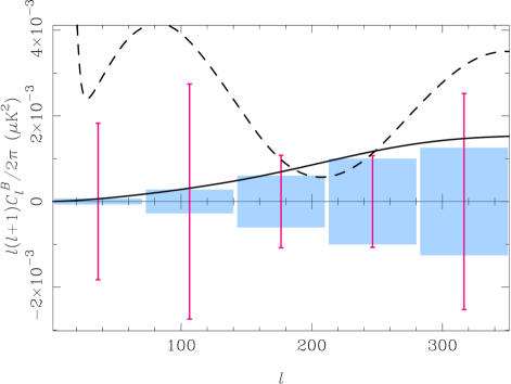
If pseudo- techniques are to be applied to future, high-sensitivity searches for gravitational waves, it is clearly desirable that the imperfect isolation of modes inherent in such methods should not compromise sensitivity to . In Fig. 10 we plot the errors on flat band-power estimates of (with ) obtained by using the unbiased estimator of Chon et al. (2004); see also the discussion in Section 2.1. The weight function applied to the -radius survey, and apodization of the correlation function, are the same as in Fig. 1. The errors are obtained from the exact covariance matrices for the pseudo-s by transforming (two-sidedly) with the appropriate pseudo-inverses and . These pseudo-inverse matrices are shown in Fig. 1. The errors are calculated for in two ways. First, we set so that we obtain the error in the recovered due to sample variance of the lensing modes. These errors are representative of what would be achieved if we were able to separate and modes perfectly, and without loss, on all scales in the maps; they agree very well with the rule of thumb in equation (147) if we swap the roles of and there. We also calculate the band-power errors obtained by setting , i.e. removing the -mode power from lensing; they agree reasonably with the rule of thumb in equation (148). These errors arise because, in any realisation, our chosen estimator receives a contribution from both and modes, despite only coupling to -mode power in the mean. Such errors can only be removed by isolating modes at the level of the map, or by adopting more optimal, non-local weighting of the data, as in maximum-likelihood power spectrum estimation. Critically, we see from Fig. 10 that the errors due to the sample variance of the modes that leak into the estimator dominate the sample variance from lensing modes on large scales, where the gravitational-wave signal resides. We conclude from the figure that pseudo- estimators will be highly non-optimal for future experiments with thermal sensitivity better than -arcmin, targeting -mode polarization over a few-hundred square degrees.666If gravitational lensing were absent, the optimal survey for detecting -mode polarization with a power spectrum of known shape but (low) unknown amplitude is a circle of radius around 10 degrees (Jaffe, Kamionkowski & Wang, 2000; , Lewis et al.2002). This assumes that the sample variance of the modes from gravitational waves does not dominate the error budget. If the lens-induced modes are treated as an additional (Gaussian) noise term, the optimal survey area is increased since sample variance becomes an issue again. The best compromise is roughly to balance the sample variance of the lens-induced modes with the thermal-noise variance. As a specific example, for 200 pairs of polarization-sensitive bolometers, with each bolometer having sensitivity , and one year of integration, a survey covering two per cent of the sky balances the thermal and sample variance.
We can make a quantitative estimate of the impact of the additional sample variance due to leaked modes on the detectability of gravitational waves as follows. To preserve all information in the pseudo-s, we bypass the step of forming unbiased estimates of [which involves the singular transformation in equation (26)], and instead estimate directly from the pseudo-s. We concatenate and into a single data vector , whose covariance matrix then consists of blocks formed from , and . We assume that all parameters except are fixed, and calculate its one-sigma Fisher error from
| (149) |
In practice, we invert the covariance matrix with a singular-value decomposition which projects out any linear dependencies in the due to the finite sky coverage. For the -radius survey, the one-sigma error on in the null hypothesis () is . Our sensitivity to improves dramatically to if we artificially set (and ) in the analysis. This latter case is representative of what could be achieved with lossless separation of the modes, followed by a pseudo- analysis of the Stokes maps of these modes. In practice, - separation is lossy, particularly on the largest scales where there is significant -mode power from reionization (, Lewis et al.2002; Bunn et al., 2003; Lewis, 2003). If we assume, crudely, that large-scale modes with are lost to the separation, we find a for the -radius survey. The effect of not isolating the modes properly in the pseudo- analysis thus degrades the limit on by a factor .
6 Conclusion
Accurate calculation of the covariance matrix is an important part of power spectrum estimation during the analysis of CMB data. A ‘correct’ estimator (i.e. unbiased), but with poorly quantified errors, is useless for subsequent parameter estimation. In this paper we have constructed the contribution from sample variance to the covariance matrices of heuristically-weighted quadratic estimates of the CMB polarization power spectra. Exact calculation of these matrices for general weighting is numerically feasible at large scales ( less than a hundred or so), but the scaling is prohibitive on small scales. To resolve this problem we developed analytic approximations to the polarization covariance matrices, including the effects of mode coupling and, in a perturbative manner, the mixing of and modes that inevitably arises with heuristic weighting. Our approximations, which generalise earlier work on the temperature anisotropies (Hinshaw et al., 2003; Efstathiou, 2004), can be computed efficiently to high . Accurate covariance matrices can be obtained on all scales by replacing the low- sectors of our approximations with a numerical calculation.
We tested the approximations against numerical results for two toy-model surveys for which azimuthal symmetry allows efficient evaluation of the exact covariances. For the more challenging survey, a -radius survey with cosine-squared apodization of the outer , the most significant errors were on the variance of . These errors arise from our local treatment of the -mode power spectrum when it appears in a convolution with the broad kernel that describes the mixing of and modes in equation (30). For the variance of (and the temperature anisotropies) the approximation is more accurate because the dominant convolution involves a kernel that is intrinsically more narrow. It will probably be very difficult to improve the error on the variance of in an analytic treatment. Fortunately, convolution errors tend to cancel in the approximation of the correlation matrices. We observed maximum errors in the correlations, except on the largest scales, suggesting that, in a practical application, it should be possible to construct accurate covariance matrices by combining the approximate correlations with variances calibrated off simulations. By binning our approximate covariances, we also derived useful rules of thumb for the variances of band-power estimates of and . These are particularly simple to evaluate, involving only integrals of products of the weight function and its derivatives.
A further aim of this paper was to quantify the conditions under which pseudo- methods can be applied to gravitational-wave searches via -mode polarization. Measurements of the -mode power spectrum from gravitational waves with future surveys with sub--arcmin thermal noise are potentially limited by the sample variance of lens-induced modes. We showed that for surveys covering one or two per cent of the sky, the additional variance due to leaked modes dominates the lensing noise. Adopting pseudo- methods would therefore by highly sub-optimal: the error on the tensor-to-scalar ratio would be times higher than if modes had been isolated before forming quadratic estimates. Ultimately, this additional variance would limit the tensor-to-scalar ratio that is detectable with pseudo- methods to . Map-level - separation, or more optimal weighting such as in maximum-likelihood power spectrum estimation, will therefore be essential to ensure the maximum returns from future -mode surveys.
Acknowledgments
ADC acknowledges a Royal Society University Research Fellowship. GC acknowledges travel support from Queens’ College, Cambridge and the Cavendish Laboratory. All theoretical power spectra in this paper were computed with CAMB (, Lewis et al.2000). Some of the results in this paper have been derived using the LAPACK777http://www.netlib.org/lapack/ package for matrix decompositions.
References
- Barkats et al. (2005) Barkats D., et al., 2005, ApJ, 619, L127
- Bartolo et al. (2004) Bartolo N., Komatsu E., Matarrese S., Rioto A., 2004, Phys. Rep., 402, 103
- (3) Bond J. R., Jaffe A. H., Knox L., 1998, Phys. Rev. D, 57, 2117
- (4) Bond J. R., Jaffe A. H., Knox L., 2000, ApJ, 533, 19
- Bunn et al. (2003) Bunn E. F., Zaldarriaga M., Tegmark M., de Oliveira-Costa A., 2003, Phys. Rev. D, 67, 3501
- Chon (2003) Chon G., 2003, PhD thesis, University of Cambridge
- Chon et al. (2004) Chon G., Challinor A., Prunet S., Hivon E., Szapudi I., 2004, MNRAS, 350, 914
- Crittenden et al. (2002) Crittenden R. G., Natarajan P., Pen U.-L., Theuns T., 2002, ApJ, 568, 20
- Efstathiou (2004) Efstathiou G., 2004, MNRAS, 349, 603
- Górski (1994) Górski K. M., 1994, ApJ, 430, L85
- Górski et al. (2004) Górski K. M., Hivon E., Banday A. J., Wandelt B. D., Hansen F. K., Reinecke M., Bartelman M., 2004, preprint (astro-ph/0409513)
- Hansen & Górski (2003) Hansen F. K., Górski K. M., 2003, MNRAS, 343, 559
- (13) Hansen F. K., Górski K. M., Hivon E., 2002, MNRAS, 336, 1304
- Hinshaw et al. (2003) Hinshaw G., et al., 2003, ApJS, 148, 135
- Hivon et al. (2002) Hivon E., Górski K. M., Netterfield C. B., Crill B. P., Prunet S., Hansen F., 2002, ApJ, 567, 2
- Jaffe, Kamionkowski & Wang (2000) Jaffe A. H., Kamionkowski M., Wang L., 2000, Phys. Rev. D, 61, 083501
- (17) Kamionkowski M., Kosowsky A., Stebbins A., 1997, Phys. Rev. Lett., 78, 2058
- (18) Kesden M., Cooray A., Kamionkowski M., 2002, Phys. Rev. Lett., 89, 011304
- Knox & Song (2002) Knox L., Song Y.-S., 2002, Phys. Rev. Lett., 89, 1303
- Kogut et al. (2003) Kogut A. et al., 2003, ApJS, 148, 161
- Kovac et al. (2002) Kovac J., Leitch E. M., Pryke C., Carlstrom J. E., Halverson N. W., Holzapfel W. L., 2002, Nature, 420, 772
- Leitch et al. (2004) Leitch E. M., Kovac J. M., Halverson N. W., Carlstrom J. E., Pryke C., Smith M. W. E., 2004, preprint (astro-ph/0409357)
- Lewis (2003) Lewis A., 2003, Phys. Rev. D, 68, 3509
- (24) Lewis A., Challinor A., Lasenby A., 2000, ApJ, 538, 473
- (25) Lewis A., Challinor A., Turok N., 2002, Phys. Rev. D, 65, 023505
- Martin & Schwarz (2000) Martin J., Schwarz D., 2000, Phys. Rev. D, 62, 103520
- (27) Mollerach S., Harari D., Matarrese S., 2004, Phys. Rev. D, 69, 063002
- Netterfield et al. (2002) Netterfield C. B., et al., 2002, ApJ, 571, 604
- Newman & Penrose (1966) Newman E., Penrose R., 1966, J. Math. Phys., 863
- Ponthieu et al. (2005) Ponthieu N., et al., 2005, preprint (astro-ph/0501427)
- Readhead et al. (2004) Readhead A. C. S., et al., 2004, Science, 306, 836
- Schulten & Gordon (1976) Schulten K., Gordon R. G., 1976, Comput. Phys. Commun., 11, 269
- Seljak & Zaldarriaga (1997) Seljak U., Zaldarriaga M., 1997, Phys. Rev. Lett., 78, 2054
- Seljak & Hirata (2004) Seljak U., Hirata C. M., 2004, Phys. Rev. D, 69, 3005
- (35) Smith K. M., Hu W., Kaplinghat, M., 2004, Phys. Rev. D, 70, 043002
- Spergel et al. (2003) Spergel D., et al., 2003, ApJS, 148, 175
- (37) Szapudi I., Prunet S., Colombi S., 2001, ApJ, 561, L11
- Tegmark & de Oliveira-Costa (2002) Tegmark M., de Oliveira-Costa A., 2002, Phys. Rev. D, 64, 063001
- (39) Varshalovich D. A., Moskalev A. N., Khersonskii V. K., 1988, Quantum Theory of Angular Momentum. World Scientific, Singapore
- (40) Wandelt B. D., Hivon E., Górski K. M., 2001, Phys. Rev. D, 64, 083003
- Zaldarriaga & Seljak (1998) Zaldarriaga M., Seljak U., 1998, Phys. Rev. D, 58, 023003
Appendix A Correlators for Gaussian-weighted and
In this appendix we derive approximate analytic expressions for the correlations between the flat-sky Fourier transforms and for a Gaussian weight function . Our expressions are valid for and large compared to . In this limit, the power spectra can be approximated as being constant over the support of ; see Section 4. Using equations (39) and (40) we can approximate the correlators by
| (150) | |||||
| (151) |
For a Gaussian weight function we can evaluate the integrals in these equations analytically; we find
| (152) | |||||
Note that
| (153) |
and the right-hand side is constructed from . This result follows quite generally from equation (41). To calculate the covariance of the errors of the power spectrum estimates we also need the following correlator
| (154) |
The integrals in this expression evaluate to
| (155) | |||||
We now have
| (156) |
and the right-hand side is constructed from . Note that if and are parallel or perpendicular.
Appendix B Useful sums of products of symbols
In Sections 2 and 4.4 we make use of a number of results for summing products of symbols. Some of these follow trivially from the orthogonality properties of the s, but others require more effort. Here, we sketch our derivation of these latter results. We make extensive use of well-known properties of the symbols, such as their symmetries and integral representations (e.g. Varshalovich et al.1988).
In Section 2 we require
| (157) |
It is the presence of the factor of , where , that complicates the evaluation of this summation. To proceed, we express the product of symbols as an integral of reduced Wigner matrices using
| (158) |
so that
| (159) |
The factor has been absorbed in reducing the product of symbols to a square. The summation over can be performed by first expressing in terms of using the recursion relations for the reduced Wigner matrices (, Varshalovich et al.1988), and then using the completeness relation. Full details can be found in Chon et al. (2004), but the final result is
| (160) |
Inserting this into equation (159) gives
| (161) |
Using the differential representation of the reduced Wigner matrices (see Section 4.3.2 of Varshalovich et al.1988), it can be shown that is a polynomial in of degree . It can thus be expanded as the series , i.e. an expansion in Legendre polynomials. Using the orthogonality of the , we see that the integral in equation (161) vanishes if . It can be performed for by replacing by its differential representation and repeatedly integrating by parts. Only boundary terms then survive, and evaluating these establishes the final result (Chon et al., 2004):
| (162) |
In Section 4.4, we require the evaluation of
| (163) |
This follows along similar lines to above. A useful intermediate result is
| (164) |
from which it follows that
| (165) |
The summation thus reduces to
| (166) |
which, again, vanishes if . Inserting the differential representation of and integrating by parts, we find
| (167) |
A further result we require in Section 4.4 is
| (168) |
Using equations (158) and (165), we find
| (169) |
In this case, is a polynomial in of degree and has a root at . It can thus be expanded as a series in with non-zero coefficients for , and so the integral in equation (169) vanishes for . The summation arises when computing band-power variances from equations (100) and (111); it occurs with prefactors and . Since we are assuming the weight function is band-limited, in , so for the contribution from vanishes. The final summation we require in Section 4.4 is
| (170) |
which reduces to
| (171) |
This time, is a polynomial in of degree that has a root at . The summation can thus be expanded in the with , so that, like , it vanishes for . The summation arises from the cross term between and in equations (100) and (111), and so this contribution to the band-power variance can also be assumed to vanish for .