Toward an Improved Analytical Description of Lagrangian Bias

Abstract

We carry out a detailed numerical investigation of the spatial correlation function of the initial positions of cosmological dark matter halos. In this Lagrangian coordinate system, which is especially useful for analytic studies of cosmological feedback, we are able to construct cross-correlation functions of objects with varying masses and formation redshifts and compare them with a variety of analytical approaches. For the case in which both formation redshifts are equal, we find good agreement between our numerical results and the bivariate model of Scannapieco & Barkana (2002; SB02) at all masses, redshifts, and separations, while the model of Porciani et al. (1998) does well for all parameters except for objects with different masses at small separations. We find that the standard mapping between Lagrangian and Eulerian bias performs well for rare objects at all separations, but fails if the objects are highly-nonlinear (low-sigma) peaks. In the Lagrangian case in which the formation redshifts differ, the SB02 model does well for all separations and combinations of masses, apart from a discrepancy at small separations in situations in which the smaller object is formed earlier and the difference between redshifts or masses is large. As this same limitation arises in the standard approach to the single-point progenitor distribution developed by Lacey & Cole (1993), we conclude that a more complete understanding of the progenitor distribution is the most important outstanding issue in the analytic modeling of Lagrangian bias.

1 Introduction

The universe is a complicated place. Not only does cosmological structure formation involve detailed questions of fluid dynamics, radiative transfer, and chemistry, but most of these issues are non-local. The impact of high-redshift supernovae (SNe), for example, is not limited to the host-galaxies in which they are born. Theoretical arguments show that the large numbers of SNe formed in high redshift dwarf galaxies drove global winds of such force that they not only reduced further infall onto their hosts, but also suppressed the formation of neighboring galaxies (e.g. Scannapieco, Ferrara, Broadhurst 2000; Thacker, Scannapieco, & Davis 2003). Observational support of this idea is strong, with large numbers of massive outflowing starbursts directly detected at $z\gtrsim 3$ (Pettini et al. 2001; Frye, Broadhurst, & Benitez 2002; Hu et al. 2002).

Such observations of outflows are complemented by hints that the intergalactic medium (IGM) surrounding high-redshift starbursts has been excavated by outflows out to distances $\sim 1$ Mpc (Adelberger et al. 2003) and that the distribution of intergalactic metals is biased and highly clustered around similar sources (Pichon et al. 2003). Furthermore, quasar absorption line studies have uncovered an inhomogeneous distribution of heavy elements that is already pervasive throughout the intergalactic medium by $z\approx 5$ (e.g. Rauch, Haehnelt, & Steinmetz 1997; Songaila 2001; Schaye et al. 2003; Aracil et al. 2003). This large-scale enrichment further complicates the structure formation process. Metal-line cooling is of crucial importance to the formation history of large galaxies (e.g. Sutherland & Dopita 1993), as low levels of enrichment can produce an order of magnitude change in cooling rates above $10^{5}$ K. Also, the presence of even trace levels of heavy elements in protogalactic material may be sufficient to drastically affect the shape of the stellar initial mass function (e.g. Bromm et al. 2001; Schneider et al. 2002).

But the most highly non-local processes are undoubtedly radiative. The earliest such example is the dissociation of primordial H${}_{2},$ which regulates the formation of the first generation of galaxies in halos with virial temperatures below $10^{4}$ K. As ${\rm H}_{2}$ is easily photo-dissociated by 11.2-13.6 eV photons to which the universe is otherwise transparent, even small numbers of forming stars have the potential to suppress dwarf galaxy formation in large regions of space (e.g. Haiman, Rees, & Loeb 1997), motivating detailed analysis of ${\rm H}_{2}$ formation by X-rays (e.g. Oh 2001) and self-shielding (Yoshida et al. 2003). Secondly, there is the question of reionization. Here the classic picture is of a two-stage process, which begins with sources ionizing their immediate surroundings and ends in a rapid “overlap” phase as H II regions join together, quickly ionizing the remaining neutral regions (e.g. Gnedin 2000). At these times feedback due to photo-evaporation is of primary importance to galaxy formation in $T_{\rm vir}=10^{4}-10^{4.5}$K halos (e.g. Barkana & Loeb 1999), a non-local effect that is only worsened by the fact that similar low-mass galaxies are likely to be the source of the ionizing background in the first place.

This wide range of mechanical, chemical, and radiative feedback processes has necessarily sparked a multifaceted numerical attack on non-local cosmological problems. Recent numerical simulations have included detailed studies of mechanical feedback from galaxy outflows (e.g. Scannapieco, Thacker, & Davis 2001; Springel & Hernquist 2003), the chemical properties of galaxies and the intergalactic medium (e.g. Thacker, Scannapieco, & Davis 2002; Theuns et al. 2002; Tassis et al. 2002) and the formation and propagation of cosmological ${\rm H}_{2}$ dissociation and ionization fronts (e.g. Ricotti, Gnedin, & Shull 2002; Ciardi, Ferrara, & White 2003; Yoshida et al. 2004). These highly non-local studies, unlike earlier investigations, are far outstripping the power of approximate analytic techniques. Thus, in our rush to match the dramatic recent observational advances in cosmology with equally sophisticated numerical work, there is a very real threat that we will soon lack the tools to understand either in a more fundamental context.

The most widely applied analytic method for determining the distribution of halos was first developed by Press & Schechter (1974, hereafter PS), and later refined by Bond et al. (1991), Lacey & Cole (1993), and Sheth, Mo, & Tormen (2001, hereafter SMT01) among others. Yet, despite its widespread utility, this method is limited in that it can only predict the average number density of virialized dark matter halos, and does not supply any information about their relative positions. However, when used in combination with simulations, this model is exceptionally useful since it allows rapid investigation of parameter space. In the absence of this possibility for studying non-local effects, numerical investigations are thus on a surprisingly shaky footing: any such investigation is computationally intensive, and is able to consider only a limited range of possible scenarios and parameters. Yet, at the same time, most processes depend on a large number of uncertain parameters, almost assuring that the simulations will not be able to bracket the full range of physically plausible scenarios. Finally, even in the cases in which simulations are able to assess these uncertainties, the lack of an analytical counterpart frequently leaves us without a basic theoretical understanding.

These limitations are somewhat mitigated by analytical studies of the two-point correlation function, although only recently have these approaches been extended to the point of being useful for feedback. Considerable effort has gone into to modeling the biased clustering of halos at a given epoch in the Eulerian coordinate system in which they are observed, both in mildly-nonlinear (see Bernardeau et al. 2002 for a review) and highly nonlinear contexts (e.g. Mo & White 1996, hereafter MW96; Seljack 2000; Ma & Fry 2000). Limited models have also been developed in the Lagrangian coordinate system in which the halos cell-centers were originally located (Porciani et al. 1998; Sheth & Lemson 1999). In this reference frame, the distance between two objects is closely related to the total mass of material between them, rather than their final comoving distance.

The usefulness of such a reference frame is twofold. Firstly, it is the natural frame for PS-type analytical calculations, which associate peaks in the initial density field with collapsed objects at various redshifts. Secondly, it allows for a more accurate treatment of the propagation of disturbances such as shocks (Scannapieco et al. 2003) or ionization fronts (Iliev et al. 2004) between objects, as these are largely dependent on the total column depth of material separating two perturbations rather than their precise distance in physical space. However, early analytical approaches were unable capture the Lagrangian clustering between halos forming at different epochs, a quantity of crucial importance to modeling non-local effects, as cosmological disturbances take a significant amount of time to propagate from their sources to neighboring objects.

In an attempt to alleviate this shortcoming, we developed in Scannapieco & Barkana (2002; hereafter SB02) an approximate analytical model that considered the collapse of two neighboring points of arbitrary mass and formation redshift, separated by an arbitrary Lagrangian distance. Working in the context of the linear excursion-set formalism of Bond et al. (1991), we showed that while the exact two-point solution could not be obtained analytically, this solution could be reproduced to high accuracy by introducing a simple approximation. The resulting expressions then interpolated smoothly between all standard analytical limits: reducing for example to the standard halo bias expression described in MW96 in the limit of equal-mass halos at the same redshift, and reproducing the Lacey & Cole (1993) progenitor distribution in the limit of different-mass halos at the same position and different redshifts.

However, just as numerical results must be placed in a larger analytical context, the analytical results obtained in SB02 were left incomplete without an accurate numerical assessment of their strengths and limitations. In this study, we carry out just such a comparison, computing detailed numerical Lagrangian halo-halo correlations at a variety of masses and redshifts and comparing them directly with SB02 and other analytical models. The structure of this work is as follows. In §2 we describe our numerical simulation and group finding techniques and compare the resulting mass distributions with standard analytical results. In §3 we systematically compare the Lagrangian correlation function of groups with the analytical model of SB02 for a variety of formation redshifts and halo masses. We conclude in §4 with a brief review of our results and a short discussion.

2 Simulations and Group Finding

To achieve high accuracy at small separations while at the same time minimizing the effects of box-mode damping, we conducted two detailed numerical simulations using a parallel OpenMP-based version of the HYDRA code (Couchman et al. 1995; Thacker & Couchman 2000). Our assumed cosmological parameters were taken to correspond to the generally accepted “concordance” values, which agree well with measurements of the Cosmic Microwave Background, the number abundance of galaxy clusters, and high-redshift supernova distance estimates (e.g. Spergel et al. 2003; Eke et al. 1996; Perlmutter et al. 1999). In this case $h=0.65$, $\Omega_{0}$ = 0.3, $\Omega_{\Lambda}$ = 0.7, $\Omega_{b}=0.05$, $\sigma_{8}=0.87$, and $n=1$, where $\Omega_{0}$, $\Omega_{\Lambda}$, and $\Omega_{b}$ are the total matter, vacuum, and baryonic densities in units of the critical density, $\sigma_{8}^{2}$ is the variance of linear fluctuations on the $8h^{-1}{\rm Mpc}$ scale, and $n$ is the “tilt” of the primordial power spectrum. We used the Bardeen et al. (1986) transfer function with an effective shape parameter of $\Gamma=0.18$.

The first run (Run A), chosen to do best at small distances, was carried out in a cubic volume $78.5$ comoving Mpc on a side, populated with $350^{3}$ dark matter particles. This run is a continuation of that used in Scannapieco & Thacker (2003). The second run (Run B), chosen to do best at large separations, was carried out in a cubic volume $113$ comoving Mpc on a side, populated with $400^{3}$ dark matter particles. The mass of each particle was $3.9\times 10^{8}{M_{\odot}}$ for Run A and $7.9\times 10^{8}{M_{\odot}}$ for Run B. Since we restrict our results to masses above $10^{11}{M_{\odot}}$ we have over 250 and 125 particles in each group used in the study. Both runs were integrated from an initial redshift of $z=49$ down to $z=1$ and used fixed physical Plummer softening lengths of 5.7 kpc (Run A) and 6.9 kpc (Run B). Both simulations were performed with 64-bit precision.

Group identification was carried out using the HOP (Eisenstein & Hut 1998) algorithm, which uses the local density for each particle to trace (“hop”) along a path of increasing density to the nearest local maximum, at which point the particle is assigned to the group defined by this maximum. Since this process assigns all particles to groups, many of these must be removed by requiring an outer threshold density, $\delta_{\rm outer}$. Finally, a “regrouping” stage is needed in which all groups are merged for which the boundary density between them exceeds $\delta_{\rm saddle}$, and all objects thus identified must have one particle whose density exceeds $\delta_{\rm peak}$ to be accepted as a final group (see Eisenstein & Hut 1998 for explicit details).

Applying these criteria with the HOP parameters $N_{\rm dens}=48$, $N_{\rm hop}=20$, $N_{\rm merge}=5$, $\delta_{\rm peak}=160$, $\delta_{\rm saddle}=140$, and $\delta_{\rm outer}=80$, yielded 1548, 4841, 6179 and 6739 groups with masses above $10^{11}{M_{\odot}}$ at redshifts $z=5$, 3, 2, and 1, respectively in Run A, and 4276, 13118, 17063,and 18424 at the same redshifts in Run B. The resulting cumulative mass functions for both runs are shown in Figure 1, where they are compared with the standard analytical PS mass function and the refined fit from the ellipsoidal collapse model of SMT01. While the PS model exhibits substantial differences from the simulation group densities, particularly for the late-forming, low-mass peaks, the SMT01 expression provides a good fit for both simulations over the full range of masses and redshifts of consideration, as has been seen in several previous comparisons (Bode 2001; Jenkins et al. 2001). Thus we expect our groups to accurately represent a “standard” sample as defined in the majority of recent N-body simulations.

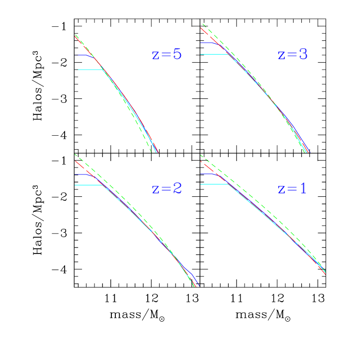
Figure 1: Comparison of numerical and analytic mass functions. Here the solid lines extending to lower masses are calculated from the simulation Run A, the solid lines that have a higher low-mass limit are calculated from simulation Run B, and the short-dashed and long-dashed lines represent the PS and the SMT01 models, respectively. Good agreement between the results of both simulations and SMT01 is found at all redshifts.

To define the Lagrangian coordinates of a group, we trace back the position of each of the particles contained within it to the start of the numerical simulation, and then compute the center of mass of this distribution. Using these positions we are then able to numerically construct $\frac{d^{2}n}{dM_{1}dM_{2}}(M_{1},z_{1},M_{2},z_{2},r)$ as described in SB02 eqs. (41) and (42), the distribution function of halos at any two given masses ($M_{1}$ and $M_{2}$), output redshift ($z_{1}$ and $z_{2}$), and initial comoving separation $r$. In practice however, it is more convenient to normalize this function by the average number of halos at each mass and redshift, defining the Lagrangian correlation function $\xi_{L}$ as the excess probability of finding two halos that are initially separated by a comoving distance $r$. That is

$$\xi_{L}(M_{1},z_{1},M_{2},z_{2},r)+1\equiv\left[\frac{d^{2}n}{dM_{1}dM_{2}}(M_{1},z_{1},M_{2},z_{2},r)\right]\left[\frac{dn}{dM_{1}}(M_{1},z_{1})\frac{dn}{dM_{2}}(M_{2},z_{2})\right]^{-1},$$ (1)

where $\frac{dn}{dM}$ is the overall distribution of halos at a single mass and redshift. It is this excess, then, that we study in detail in the comparisons presented below.

3 Comparisons with Analytics

3.1 Single Redshift, Single Mass

In order to study the behavior of the Lagrangian correlation function over a range of masses, we divided our sample of groups into 3 bins at each redshift, containing objects of total mass $10^{11}{M_{\odot}}\leq M<10^{11.5}{M_{\odot}}$, $10^{11.5}{M_{\odot}}\leq M<10^{12}{M_{\odot}}$, and $10^{12}{M_{\odot}}\leq M<10^{12.5}{M_{\odot}}$. While the central values in each of these bins are $10^{11.25}{M_{\odot}}$, $10^{11.75}{M_{\odot}}$, and $10^{12.25}{M_{\odot}}$ respectively, we see from the steep mass functions in Figure 1 that the majority of groups in each bin are dominated by the smallest values. In fact, for all bins and redshift ranges considered here, the mean is well approximated by the minimum value plus a third of the width. Thus, throughout this study, we refer to these subsets as bins of mass $10^{11.15}{M_{\odot}}$, $10^{11.65}{M_{\odot}}$, and $10^{12.15}{M_{\odot}}$, comparing them with analytic results for these values.

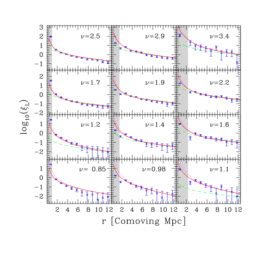
Figure 2: Lagrangian correlation function of objects with the same mass at the same redshift. From top to bottom $z=5$, $z=3$, $z=2$, and $z=1$, and from left to right the mass bins are centered on $10^{11.15}{M_{\odot}},$ $10^{11.65}{M_{\odot}}$ and $10^{12.15}{M_{\odot}}$. The points are the simulation values, the solid lines are the SB02 model, the dotted lines are the Porciani et al. (1998) model and the dashed lines are the simple MW96 geometric bias estimates. The shaded regions are within the (spherical) radius of the halo as defined by eq. 7 .We omit the MW96 estimate in cases in which $\nu\leq 1$.

Constructing $\xi_{L}$ for each of these mass bins and redshifts resulted in the points depicted in Figure 2, in which we have taken a bin width of 1 Mpc. We have computed error bars including both the standard (Poissonian) error, which depends on the number of pairs in a given bin, as well as the additional scatter caused by the finite sample size used to construct the correlation function. In this case the variance in the number of pairs in a given bin $i$ in a single simulation is well-approximated by

$$\sigma^{2}(N_{i,1,2})=N_{i,1,2}+N_{i,1,2}^{2}\left[\frac{2}{N_{1}}+\frac{2}{N_{2}}\right],$$ (2)

where $N_{i,1,2}$ is the number of pairs in a bin $i$, while $N_{1}$ and $N_{2}$ are the total numbers of objects of each of the two types being measured (Mo, Jing, & Börner 1992). Thus combining two measurements of $\xi_{L}$ with relative weights $w^{A}$ and $w^{B}$ leads to a total error in each bin $i$ and objects types $1$ and $2$ of

$$\sigma^{2}(\xi^{\rm Tot}_{L,i,1,2})=(w^{A}_{1,2})^{2}(\xi^{A}_{L,i,1,2}+1)^{2}\sigma^{2}(N^{A}_{i,1,2})+(w^{B}_{1,2})^{2}(\xi^{B}_{L,i,1,2}+1)^{2}\sigma^{2}(N^{B}_{i,1,2}),$$ (3)

where we choose our weights based on the total number of pairs with masses 1 and 2 in each simulation at any given output $z$:

$$w^{A}_{1,2} = N^{A}_{1}N^{A}_{2}/(N^{A}_{1}N^{A}_{2}+N^{B}_{1}N^{B}_{2}),$$

$$w^{B}_{1,2} = N^{B}_{1}N^{B}_{2}/(N^{A}_{1}N^{A}_{2}+N^{B}_{1}N^{B}_{2}).$$ (4)

Each panel in Figure 2 is labeled by its “density threshold,” $\nu$, a value that arises in the analytical mass functions. This is defined as

$$\nu\equiv 1.69D(z)^{-1}\sigma(M)^{-1},$$ (5)

where $D(z)$ is the linear growth factor. The density threshold can then be used to construct a standard “geometrical bias” estimate of the correlation function:

$$\xi_{L}(M_{1},z_{1},M_{2},z_{2},r)\approx b_{L}(M_{1},z_{1})b_{L}(M_{2},z_{2})D(z_{1})D(z_{2})\xi_{\rm DM}(r),$$ (6)

where $b_{L}\equiv(\nu^{2}-1)/1.69$ and $\xi_{\rm DM}$ is the underlying matter correlation function, linearly extrapolated to the present epoch (e.g. Kaiser 1984; MW96). For reference this estimate of $\xi_{L}$ is shown as the short-dashed lines in each panel, while the solid lines give the more detailed model developed in SB02. Finally, the dotted lines are from the model described in eq. (A1) of Porciani et al. (1998; hereafter P98), which is similar to SB02, but applicable only in the case of two halos with the same collapse redshift.

Surveying this figure, we see that, in general, there is good agreement between the SB02 model and the numerical results at all masses and redshifts. Furthermore, in the case of $M_{1}=M_{2}$ the P98 model is nearly equivalent to this expression, and thus obtains similar agreement. On the other hand, the standard MW96 model, which was derived in the limited case of large separations and high values of $\nu$, is not able to trace $\xi_{L}$ within a distance of $\sim 4$ comoving Mpc, or $\nu$ values less than 1.5. Note that for $\nu<1$ the MW96 model becomes negative, and thus we omit this simple estimate for these cases.

Even in the more detailed SB02 model, a minor discrepancy is seen, namely a deficit in the numerical results in the 1-2 Mpc bins. The difference is most noticeable in the $10^{12.15}{M_{\odot}}$ case, where the 2 Mpc bin is missing from all plots. The explanation of this phenomenon is straightforward and arises from the group finding process. For our chosen cosmology, a (spherical) Lagrangian region that encompasses a mass $M$, will have a comoving radius, $R_{L}(M)$, that is given by

$$R_{L}(M)=1.9\,\left[M/(10^{12}{M_{\odot}})\right]^{1/3}\qquad{\rm Mpc}.$$ (7)

Thus in the $10^{12.15}{M_{\odot}}$ plot the entire second bin is contained within the value of $R_{L}$, while for the $10^{11.65}{M_{\odot}}$ case approximately half of the bin is contained within $R_{L}$. It is clear that the deficit is caused by the fact that HOP, like any group-finding algorithm, will consider objects at these separations as a single higher-mass group, excluding them from the numerical calculation of $\xi_{L}$. Note that the correlation function at $0$ separation is formally infinite, as an object of mass $M$ at a redshift $z$ is always found at a distance of $r=0$ from an object of similar mass and redshift (namely itself). This means that the innermost bin is also not interesting for our purposes.

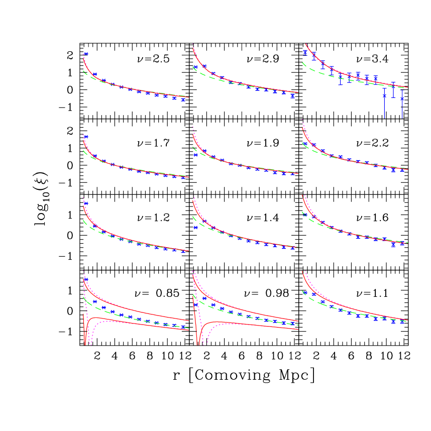
Figure 3: Eulerian correlation function of objects with the same mass at the same redshift. Panels are as in Figure 2. The points are the simulation values, and the dashed lines are the simple MW96 Eulerian geometric bias estimates. The solid and dotted lines are the SB02 and P98 models as mapped to Eulerian coordinates as described in the text. In the cases in which $\nu\leq 1,$ both possible values for $b_{E}$ as in eq. (8) are shown.

To compare our simulations with more standard estimates we plot the Eulerian correlation function in comoving coordinates, for objects with the same mass and redshift, in Figure 3. In this case the bias factor that appears in the MW96 estimate is modified to $b_{E}=(\nu^{2}-1)/1.69+1=b_{L}+1$ to account for the motion of the halos toward each other. We find good agreement between the estimates and numerical values at large separations, as has been previously studied in detail (e.g. Jing 1998), again giving us confidence in our numerical sample.

In a numerical study of several $256^{3}$ simulations, Jing (1999) found that the $b_{E}=b_{L}+1$ mapping between Eulerian and Lagrangian coordinates provided a good fit to these correlation functions at large distances. Furthermore, he conjectured that the nonlinear effect in the mapping between coordinate systems was not a major source of the inaccuracy of the MW96 formula. To test this conjecture in the context of our analytical modeling, we have also plotted in Figure 3 the bias estimated as

$$b_{E}(z,r)=1\pm\sqrt{{\rm abs}[\xi_{L}(r)D(z)^{-2}\xi_{\rm DM}(r)^{-1}]},$$ (8)

where $\xi_{L}(r)$ is the Lagrangian correlation function as calculated by SB02 or P98, and the $\pm$ sign is taken to be positive if $\nu\geq 1$ and negative if $\nu<1$. Disregarding the innermost bin, we find that for the $z=5$, 3, and 2 results, this conjecture indeed seems to hold. As $\nu$ approaches, and then falls below 1 however, this approximation breaks down. Thus a more sophisticated Eulerian to Lagrangian mapping is likely to be necessary to reproduce the behavior of these correlation functions at small separations (as in e.g. Iliev et al. 2003).

3.2 Single Redshift, Two Masses

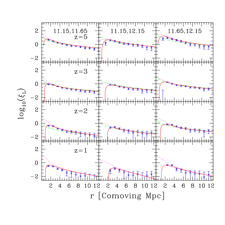
Figure 4: Lagrangian correlation function of objects with different masses at the same redshift. From top to bottom $z=5$, $z=3$, $z=2$, and $z=1$, and from left to right the mass bin pairs are centered on ($10^{11.15}{M_{\odot}}$, $10^{11.65}{M_{\odot}}$), ($10^{11.15}{M_{\odot}}$, $10^{12.15}{M_{\odot}}$), and ($10^{11.65}{M_{\odot}}$, $10^{12.15}{M_{\odot}}$), respectively. Lines and points are as in Figure 2, with the MW96 estimate omitted if $\nu\leq 1$.

Next we turn our attention to the case of two dark matter halos with different masses. In Figure 4 we plot the correlation function for mass bin pairs ($10^{11.15}{M_{\odot}}$,$10^{11.65}{M_{\odot}}$), ($10^{11.15}{M_{\odot}}$,$10^{12.15}{M_{\odot}}$) and ($10^{11.65}{M_{\odot}}$,$10^{12.15}{M_{\odot}}$) at our chosen redshifts. As in the single-mass case, all analytical approaches do well at large separations and high $\nu$ values. Also as in the single-mass case, the MW96 result fails when $\nu(M,z)$ approaches 1 for either of the halos under comparison, while the P98 and SB02 results are able to handle this range of parameters. Unlike the single mass case, however, only the SB02 model is able to reproduce the behavior at small separations. This is because at these distances the MW96 model is too simplified, while the P98 model does not correctly implement the “barriers” that exclude the formation of a density peak within a larger peak in the excursion set formalism (Bond et al. 1991). Indeed in Figure 3 of P98, the authors point out that their approximation fails to reproduce the exact excursion-set solution at separations $r\lesssim 5R_{L}(M),$ with $R_{L}$ defined as in eq. (7). These barriers are properly accounted for, however, in the SB02 model, and thus the presence of two objects of different masses at the same position and redshift is excluded in this formalism.

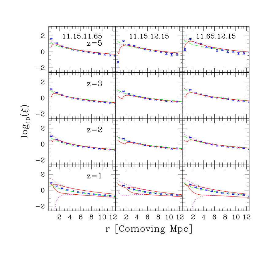
Figure 5: Eulerian correlation function of objects with different masses at the same redshift. Panels are as in Figure 4. The points are the simulation values, and the dashed lines are the simple MW96 Eulerian geometric bias estimates. The solid and dotted lines are the SB02 and P98 models as mapped to Eulerian coordinates as described in the text. In the $z=1$ cases both possible values for $b_{E}$ as in eq. (8) are shown.

In Figure 5 we compare the Eulerian correlation functions measured in our simulations with the ($b_{E}=\nu^{2}-1/1.69+1$) MW96 estimates and the P98 and SB02 estimates as mapped to this coordinate system by eq. (8). As in Figure 4, all models do well at large separations, when $\nu>1$. Unlike the Lagrangian case, however, no exclusion is seen in the numerical results at small separations. As collapse and virialization decrease the radius of a perturbation by a factor $\sim 1/6$, there is nothing preventing two objects whose initial centers of mass were quite separated from moving together to very close distances. Thus the Eulerian version of the SB02 model is a poor approximation at these separations, while the P98 and MW96 models, which do not impose this exclusion, do as well in most cases. In fact, the MW96 model, despite its simplicity, provides the best overall fit to the data, while both of the more sophisticated models fail at $z=1.$ While this agreement provides us a simple approximation in Eulerian space, it again serves to point out that the relationship between Eulerian and Lagrangian spaces is complex for low $\nu$ values and small distances.

3.3 Two Redshifts, Single Mass

While the single redshift comparisons above give us good confidence in our analytical modeling of simultaneously collapsing halos, this case is only of secondary importance for non-local effects in structure formation. In reality, cosmological disturbances such as ionization fronts and outflows take an appreciable amount of time to propagate from their sources to neighboring objects. In fact, the majority of feedback effects are most efficient if they reach the neighboring perturbations before they have virialized (e.g. Haiman, Rees, & Loeb 1997; Scannapieco, Ferrara, Broadhurst 2000). Thus it is essential that any analytical treatment of non-local effects in structure formation be capable of adequately handling these cases.

Two-redshift correlation functions are not unknown observationally. The positions of galaxies measured at a redshift $z_{1}$ can in principle be correlated with the positions of galaxies at an earlier redshift $z_{2}.$ However, for both objects to be observed simultaneously and not be behind each other, $r>c[t(z_{1})-t(z_{2})],$ meaning that the light from the $z_{2}$ galaxy (as we see it today) is unable to reach the $z_{1}$ galaxy (as we observe it). In fact, such distances are long indeed, $\gtrsim 1000$ comoving Mpc for our output times, and well beyond our ability to simulate. Instead we concentrate here on distances $r\ll c[t(z_{1})-t(z_{2})]$ which, while not directly observable, are much more typical for the propagation of cosmological disturbances.

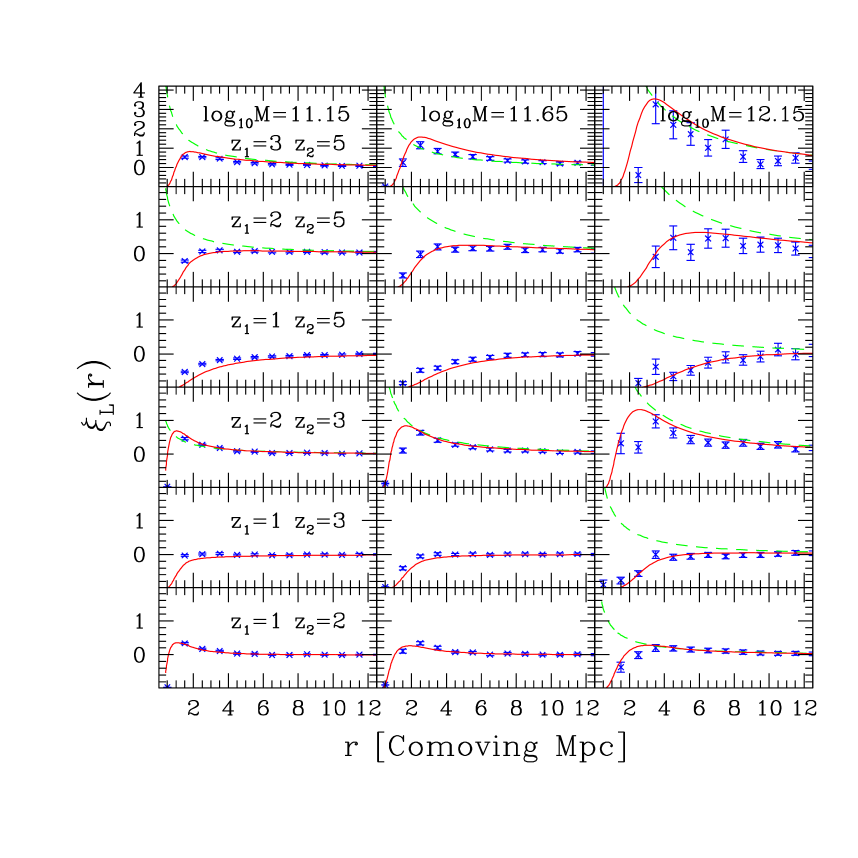
Figure 6: Lagrangian correlation function of objects with the same mass, at different redshifts. Each row is labeled by its $z$ values and each column is labeled by its $M$ value. In all panels the solid lines are the SB02 model, and the dashed lines are the MW96 model in the cases in which $\nu\geq 1$ for both halos. Note that we plot $\xi_{L}$ rather than $\log_{10}(\xi_{L})$ as the correlation function becomes negative at small separations.

In Figure 6, we again consider two halos with the same mass, but now with different collapse redshifts. At large separations, the numerical values display much the same behavior as in Figure 2. The correlation between halos is stronger for rarer objects, and weaker for smaller masses and later redshifts. Hence it is not surprising that both the MW96 and SB02 models do well at reproducing these trends, although again, only the SB02 model is applicable if either $\nu_{1}$ or $\nu_{2}\leq 1.$ (The P98 model is omitted here as it was constructed only at a single redshift.)

At smaller separations, the two-redshift case differs significantly from the behavior seen in Figure 2. As it is impossible for an object to have exactly the same mass at two significantly different redshifts, each of the numerical values approaches $\xi_{L}=-1$ at small separations. Thus, just as the MW96 model underestimates the (formally infinite) small-distance clustering of two halos of the same mass and redshifts, it vastly overestimates the small-distance clustering of two halos with the same mass and different $z$ values. On the other hand, the SB02 model is constructed so as to exclude the formation of a halo of the same mass at the same position at multiple redshifts, and thus the resulting curves turn over at small separations, following the simulation. In fact, good agreement is seen at all separations, masses and redshifts, with the possible exception of a slight underestimate in the cross correlation between low mass $z_{1}=1$ halos and those at $z_{2}=5$, a comparison which includes both the most nonlinear (lowest $\nu$ value) peaks and the largest offset between $z_{1}$ and $z_{2}$.

3.4 Two Redshifts, Two Masses

Finally, we turn our attention to the most difficult case to model analytically, the correlation between two objects that differ both in mass and formation redshift. First we consider the case in which the smaller object forms at a higher redshift. This is essentially a generalization of the progenitor problem, in which one is interested in the probability that an object of mass $M_{\rm progen}$ was found at a redshift $z_{\rm progen}$ at a position at which an object with a mass $M_{\rm final}$ is known to exist at a redshift $z_{\rm final}$. This distribution was first constructed analytically in the context of the Bond et al. (1991) excursion set formalism by Lacey & Cole (1993), in what has now become a standard approach. As the SB02 model was also developed within this context, it matches this model exactly at $r=0$, as is clear from Figure 7.

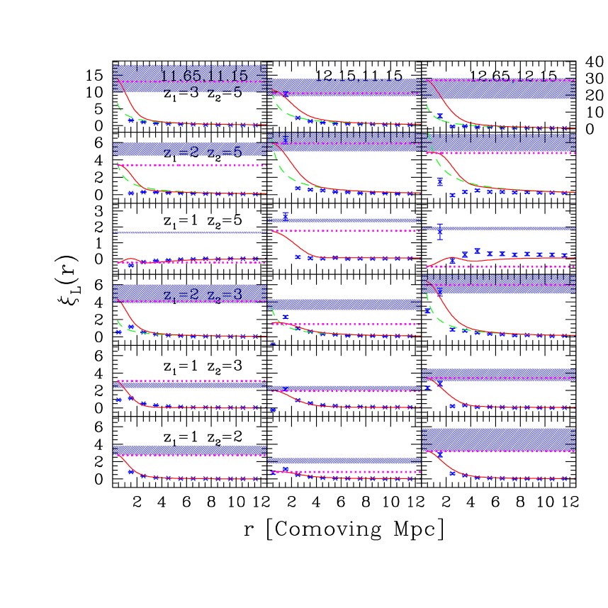
Figure 7: Lagrangian correlation function of objects with different masses and redshifts, with the smaller mass at the higher redshift. In this figure, the points are the simulation results, the dashed and solid curves are the MW96 and SB02 models, and the horizontal dotted lines are the $r=0$ estimates as given by the Lacey & Cole (1993) progenitor distribution. Finally, the shaded bands are the range of progenitor number densities measured from the simulations, as described in §3.4. Each row is labeled by its $z$ values and each column (from left to right) corresponds to mass bins centered on ($10^{11.15}{M_{\odot}}$, $10^{11.65}{M_{\odot}}$), ($10^{11.15}{M_{\odot}}$, $10^{12.15}{M_{\odot}}$), and ($10^{11.65}{M_{\odot}}$, $10^{12.15}{M_{\odot}}$). The $y$-axis label on the right only applies to the upper panel at the extreme right.

Also in this figure, we see that the SB02 expression does well at larger separations for all combinations of masses and redshifts. At small separations, however, a significant discrepancy is seen. As in Figure 2, this is primarily due to pushing our comparison into separations in which $r\leq R_{L}(M).$ At these short distances, our numerical and analytical approaches are essentially calculating different quantities. From a numerical perspective, our choice of bins with a 1 Mpc width means that changes in the position of the Lagrangian center of mass of the smaller object within the larger object are able to move power between the leftmost bins. On the other hand, the analytical estimates are constructed to reproduce the total number of $M_{2}$ halos merging into $M_{1}$, regardless of where they lie within the final object. Thus a fair comparison between our analytical and numerical results can only be carried out by choosing an inner bin-width that is representative of the size of final halo.

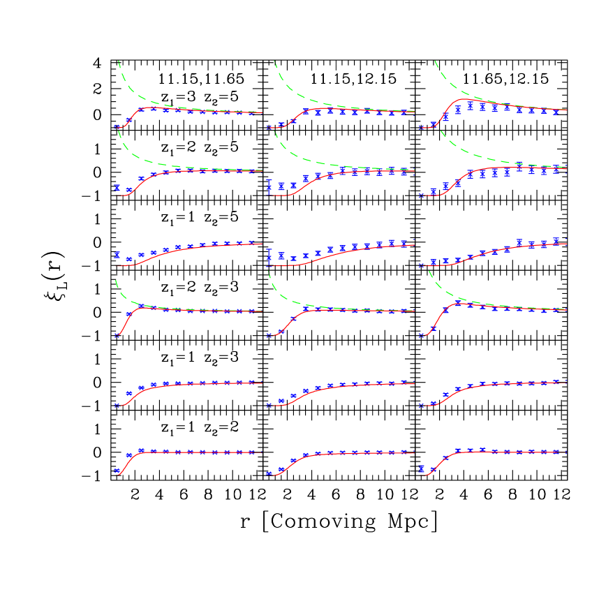
Figure 8: Lagrangian correlation function of objects with different masses and redshifts, with the larger mass at the higher redshift. Rows and columns are as in Figure 7.

As there is some flexibility in this definition, we recalculated the numerical correlation function at zero separation over a range of bin-widths from $R_{L}(M_{1})$ to $R_{L}(M_{1})+R_{L}(M_{2})/2,$ where $M_{1}$ is the mass of the larger halo. The resulting range of $\xi_{L}(0)$ values are represented by the shaded regions in Figure 7. In general the larger the bin-width, the weaker the overall correlation function. Thus, for example, the $z_{1}=3$, $z_{2}=5$, $M_{1}=10^{11.65}{M_{\odot}}$, $M_{2}=10^{11.15}{M_{\odot}}$ model attains $\xi_{L}(0)$ values of 18.7 to 10.1 over the range of bin-widths from $1.5$ to $2.0$ comoving Mpc respectively. Comparing these with the Lacey & Cole (1993) estimates we find that our numerical results are generally in agreement if the difference between redshifts and masses is small. For larger differences in mass and redshift, however, significant discrepancies exist between these approaches, and there is no obvious trend with mass and redshift that might suggest an underlying relationship in the results.

Similar inaccuracies have been observed elsewhere in the literature. For example in Somerville et al. (2000) (Fig 2), differences of $\sim 2$ between the analytical and numerical results are seen in cases in which $D(z_{1})/D(z_{2})\sim 2$ or $M_{1}/M_{2}\gtrsim 3,$ while order of magnitude discrepancies can arise if $D(z_{1})/D(z_{2})\geq 3.$ Thus the trends seen in this figure represent the limitations of pushing the standard progenitor expression outside of the $M_{1}/M_{2}$ and $D(z_{1})/D(z_{2})$ ranges in which it was originally tested (Lacey & Cole 1994). Clearly more sophisticated models for progenitor distributions are necessary to reproduce this behavior (e.g. Manrique et al. 1998; Chiueh & Lee 2001; Sheth & Tormen 2002; Sheth 2003).

In Figure 8 we consider the inverse progenitor problem, assigning an earlier formation redshift to the object with the greater mass. As gravitation is only able to increase the mass of any structure with time, this means that no such pair can exist at $r=0$ and thus $\xi_{L}$ must approach $-1$ at small separations. In this case, the subtle $r=0$ behavior seen in Figure 7 is replaced by simple exclusion, and the simulated results are well reproduced by the SB02 model for all choices of parameters. As this turn-over requires $\xi_{L}(r)/\xi_{\rm DM}(r)$ to vary with radius, the simple MW96 estimates are unable to reproduce this behavior, and thus are widely discrepant for small $r$ values.

4 Conclusion

Despite the widespread use of single-point “merger-tree” approaches in analytical studies of galaxy formation, nonlocal processes abound in cosmology. Starburst galaxies have drove winds strong enough to strip the gas out of neighboring density perturbations. The resulting inhomogeneous enrichment of the IGM profoundly affected the cooling properties of later-forming galaxies, perhaps altering their stellar initial mass function. The ultraviolet radiation from the earliest objects strongly inhibited the formation of similar such sources. Indeed, the moment the universe emerged from the cosmological “dark ages” it was plunged into an era of strong, nonlocal feedback that continues to this day.

In this study, we have used high-resolution N-body simulations to examine the Lagrangian dark-matter halo correlation function, a quantity that is uniquely suited to studying nonlocal processes because: (1) it is in the natural coordinate systems for PS-type analytical calculations; (2) it allows for a more accurate treatment of the propagation of cosmological disturbances, which are largely dependent on the total column depth of material separating two perturbations. Comparing our results with a number of analytic expressions, we find that the bivariate mass function derived in SB02 can be used to accurately reproduce the Lagrangian correlation function of halos with different masses and formation redshifts. This is a significant step forward, which confirms that non-local processes can be modeled within the framework of the bivariate mass function.

In the case of single mass, single redshift halos, the SB02 model and the P98 model both reproduce the correlation function behavior well. As expected we confirm the failure of the MW96 model for low $\nu$ and small radii ($r<4$ Mpc), but the $b_{E}=b_{L}+1$ mapping proposed by Jing works well for all masses and radii, unless $\nu$$\;\buildrel<\over{\sim}\;$$1.5$. At this point the mapping breaks down, and a more sophisticated technique is needed to deal with the short-range physics that comes into play.

For objects of different masses at the same redshift, the P98 model and the SB02 model have close agreement to a limiting radius that is defined by the turn-over in the correlation function due to the anticorrelation required at zero separation. The P98 model does not correctly reproduce this turn-over, due to the omission of the appropriate barrier treatment for the formation of structure within peaks, while the SB02 model exhibits the correct short-range behavior for all our studied cases of different masses and redshifts.

The different mass, same redshift Eulerian correlation functions for the SB02 and P98 models exhibit similar performance issues to the same mass, same redshift comparison. The problems are particularly acute for the SB02 model where the barrier treatment introduces a strong kink in the Eulerian correlation function. In these cases, remarkably, the Eulerian MW96 model works best of all three models.

The two redshift, equal mass Lagrangian case also shows the SB02 model to perform well. The growth of halo mass with redshift forces anticorrelation of equal mass halos at different redshifts and small radii. The correct turnover in the correlation function for small radii is observed, and the position of the knee is accurately predicted for all redshift cases.

Unsurprisingly, our most interesting results come from the most difficult case to study, namely the correlation of halos with different masses and formation redshifts. In the case in which the larger mass is at the higher redshift, the SB02 model reproduces the expected anticorrelation extremely accurately. In the more relevant case of the lower mass at higher redshift the Lacey & Cole (1993) progenitor distribution is always reproduced exactly at small radii, and this distribution compares well with the simulations, provided that the differences in redshift and mass between the halo are not too large ($M_{2}/M_{1}<10$ and $z_{1}-z_{2}<3$). For larger differences in mass and redshift, however, both the Lacey & Cole (1993) and SB02 models exhibit significant discrepancies from the numerical values measured here and reported elsewhere. At larger radii, however, the SB02 model reproduces the expected behavior of the correlation function in all cases. It is intriguing that the single-point case remains the single most important outstanding issue in our analytic modeling of Lagrangian bias.

- (1)
- (2) Aracil, B. Petitjean, P., Pichon, C., & Bergeron, J. 2004, A&A, 419, 881
- (3) Bardeen, J. M., Bond, J. R., Kaiser, N., & Szalay, A. S. 1986, ApJ, 304, 15
- (4) Barkana, R. & Loeb, A. 1999, ApJ, 523, 54
- (5) Bernardeau, F., Colombi, S., Gaztañaga, E., & Scoccimarro, R. 2002, Phys. Rep. 367, 1
- (6) Bode, P., Ostriker, J. P., & Turok, N. 2001, ApJ, 556, 93
- (7) Bond, J. R., Cole, S., Efstathiou, G., & Kaiser, N. 1991, ApJ, 379, 440
- (8) Bromm V., Ferrara, A., Coppi P.S., & Larson, R. B. 2001, MNRAS, 328, 969
- (9) Chiueh, T. & Lee, J. 2001, ApJ, 555, 83
- (10) Ciardi, B., Ferrara, A., & White, S. D. M. 2003, MNRAS, 334, L7
- (11) Couchman, H. M. P., Thomas, P. A., & Pearce, F. R. 1995, ApJ, 452, 797
- (12) Eisenstein, D. J. & Hut, P. 1998, ApJ, 498, 137
- (13) Eke, V. R., Cole, S., & Frenk, C. S. 1996, MNRAS, 282, 263
- (14) Frye, B., Broadhurst, T., & Benitez, N. 2002, ApJ, 568, 558
- (15) Gnedin, N. Y. 2000 ApJ, 535 530
- (16) Haiman, Z., Rees, M. J., & Loeb, A. 1997, ApJ, 484, 985
- (17) Hu, E. M., et al. 2002, ApJ, 568, L75
- (18) Iliev, I. T., Scannapieco, E., Martel, H., & Shapiro, P. R. 2003, MNRAS, 341, 8
- (19) Iliev, I. T., Scannapieco, E., & Shapiro, P. R. 2004, ApJ, submitted
- (20) Jenkins, A. et al. 2001, MNRAS, 321, 372
- (21) Jing, Y. P. 1998, ApJ, 503, L9
- (22) Jing, Y. P. 1999, ApJ, 515, L45
- (23) Kaiser, N. 1984, ApJ, 284, L9
- (24) Lacey, C. G. & Cole, S. 1993, MNRAS, 262, 627
- (25) Lacey, C. G. & Cole, S. 1994, MNRAS, 271, 676
- (26) Ma, C.-P. & Fry, J. N. 2000, ApJ, 531, L87
- (27) Manrique., A., Raig A., Solanes J., Gonzalez-Casado G., Stein, P., Salvador-Solé, E. 1998, ApJ, 499, 548
- (28) Mo, H. J., Jing, Y. P., & Börner, G. 1992, ApJ, 392, 452
- (29) Mo, H. J. & White S. D. M. 1996, MNRAS, 282, 348 (MW96)
- (30) Oh, S. P. 2001, ApJ, 553, 449
- (31) Perlmutter, S., et al. 1999, ApJ, 517, 565
- (32) Pettini, M., Steidel, C. C., Adelberger, K. L., Dickinson, M., & Giavalisco, M. 2001, ApJ, 528, 96
- (33) Pichon, C., Scannapieco, E., Aracil, B., Petitjean, P., Aubert, D., Bergeron, J., & Colombi, S. 2003, ApJ, 597, L97
- (34) Porciani, C., Matarrese, S., Lucchin, F., & Catelan, P. 1998, MNRAS, 298, 1097 (P98)
- (35) Press, W. H., & Schechter, P. 1974, ApJ, 187, 425 (PS)
- (36) Rauch, M., Haehnelt, M.G., & Steinmetz, M. 1997, ApJ, 481, 601
- (37) Ricotti, M., Gnedin, N. Y., & Shull, J. M. 2002, ApJ, 575, 49
- (38) Scannapieco, E., Ferrara, A., & Broadhurst, T. 2000, ApJ, 536, L11
- (39) Scannapieco, E., & Barkana, R. 2002, ApJ, 571, 585 (SB02)
- (40) Scannapieco, E., & Thacker R. J. 2003, ApJ, 590, L69
- (41) Scannapieco, E., Schneider, R., & Ferrara, A. 2003, ApJ, 589, 35
- (42) Schaye, J., Aguirre, A., Kim T.-S., Theuns, T., Rauch, M., & Sargent, W. L. W. 2003, ApJ, 596, 768
- (43) Schneider, R., Ferrara, A., Natarajan, P., & Omukai, K. 2002, ApJ, 571, 30
- (44) Seljack, U. 2000, MNRAS, 318, 203
- (45) Sheth, R. L., & Lemson, G. 1999, MNRAS, 304, 767
- (46) Sheth, R. L., Mo, H. J., & Tormen, G. 2001, MNRAS, 323, 1 (SMT01)
- (47) Sheth, R. L. & Tormen, G. 2002, MNRAS, 329, 61
- (48) Sheth, R. L. 2003, MNRAS, 345, 1200
- (49) Somerville, R S., Lemson, G., Kolatt, T. S., & Dekel, A. 2000, MNRAS, 316, 479
- (50) Songaila, A. 2001, ApJ, 561, L153
- (51) Springel, V. & Hernquist, L. 2003, ApJ, 339, 278
- (52) Spergel, D. N., et al. 2003, ApJS, 148, 175
- (53) Sutherland, R. S., & Dopita, M. A. 1993, ApJS, 88, 253
- (54) Tassis, K., Abel, T., Bryan, G. L., & Norman, M. L. 2002, ApJ, 587, 13
- (55) Thacker, R. J., & Couchman, H. M. P. 2000, ApJ, 545, 728
- (56) Thacker, R. J., Scannapieco, E., & Davis, M. 2002, ApJ, 581, 836
- (57) Yoshida, N., Abel, T., Hernquist, L., & Sugiyama, N. 2003, ApJ, 592, 645
- (58) Yoshida, N., Bromm, V., & Hernquist, L. 2004, ApJ, 605, 579
- (59)