Unveiling the composition of radio plasma bubbles in galaxy clusters with the Sunyaev-Zel’dovich effect

The Chandra X-ray Observatory is finding a large number of cavities in the X-ray emitting intra-cluster medium which often coincide with the lobes of the central radio galaxy. We propose high-resolution Sunyaev-Zel’dovich (SZ) observations in order to infer the still unknown dynamically dominating component of the radio plasma bubbles. This work calculates the thermal and relativistic SZ emission of different compositions of these plasma bubbles while simultaneously allowing for the cluster’s kinetic SZ effect. As examples, we present simulations of an Atacama Large Millimeter Array (ALMA) observation and of a Green Bank Telescope (GBT) observation of the cores of the Perseus cluster and Abell 2052. We predict a 5$\sigma$ detection of the southern radio bubble of Perseus in a few hours with the GBT and ALMA while assuming a relativistic electron population within the bubble. In Abell 2052, a similar detection would require a few ten hours with either telescope, the longer exposures mainly being the result of the higher redshift and the lower central temperature of this cluster. Future high-sensitivity multi-frequency SZ observations will be able to infer the energy spectrum of the dynamically dominating electron population in order to measure its temperature or spectral characteristics. This knowledge can yield indirect indications for an underlying radio jet model.

1 Introduction

The Chandra X-ray Observatory is detecting numerous X-ray cavities in clusters of galaxies confirming pioneering detections of the ROSAT satellite. Prominent examples include the Perseus cluster (Böhringer et al. 1993; Fabian et al. 2000), the Cygnus-A cluster (Carilli et al. 1994), the Hydra-A cluster (McNamara et al. 2000), Abell 2597 (McNamara et al. 2001), Abell 4059 (Huang & Sarazin 1998; Heinz et al. 2002), Abell 2199 (Fabian 2001), Abell 2052 (Blanton et al. 2001), the vicinity of M84 in the Virgo cluster (Finoguenov & Jones 2001), the RBS797 cluster (Schindler et al. 2001), and the MKW3s cluster (Mazzotta et al. 2002). They are produced by the release of radio plasma from active galactic nuclei (AGN) which are typically hosted by a cD galaxy located at the cluster center and mainly reside within the cool cores of galaxy clusters.

While radio synchrotron emission provides evidence for the existence of cosmic ray electrons (CRes) and magnetic fields, the detailed composition of the plasma bubble governing its dynamics is still unknown. Minimum energy or equipartition estimates of the nonthermal pressure in the radio bubbles give values which are typically a factor of ten smaller than the pressures required to inflate and maintain the bubbles as determined from the surrounding X-ray gas (e.g., Blanton et al. 2001). This indicates that the standard minimum energy or equipartition radio arguments are missing the main component of the pressure and energy content of the radio lobes. Possibilities include magnetic fields, cosmic ray proton (CRp) or CRe power-law distributions, or very hot thermal gas. Solving this enigma would yield further insight into physical processes within cool cores (De Young 2003) as well as provide hints about the composition of relativistic outflows of radio galaxies because plasma bubbles represent the relic fluid of jets (e.g. Celotti et al. 1998; Hirotani et al. 1998; Sikora & Madejski 2000).

Additionally, some of the clusters exhibit cavities in the X-ray emitting intra-cluster medium (ICM) without detectable high frequency radio emission, for instance in Perseus, Abell 2597, Abell 4059, and the MKW3s cluster. This category of X-ray cavities is also believed to be filled with radio plasma, but during the buoyant rise of the light radio plasma bubble in the cluster’s potential (Gull & Northover 1973; Churazov et al. 2000, 2001; Brüggen & Kaiser 2001) the resulting adiabatic expansion and synchrotron/inverse Compton losses dwindles the observable radio emitting electron population producing a so-called ghost cavity or radio ghost (Enßlin 1999). Possible entrainment of the ICM into the plasma bubble and subsequent Coulomb heating by CRes generates further uncertainty of the composition of the ghost cavity.

If the radio bubbles contain a significant amount of very hot thermal gas, this might be detected by X-ray observations. However, this is quite difficult (e.g., Blanton et al. 2003) due to the projected foreground and background cluster emission, and the fact that the X-ray emissivity is proportional to the square of the density. If most of the pressure in the radio bubbles were due to the very hot, low density thermal gas, it would have a very low X-ray emissivity. Observationally, there has been a claim by Mazzotta et al. (2002) to have seen hot X-ray emitting gas within the ghost cavity of the MKW3s cluster. Obviously, it might be more useful to observe the radio bubbles with a technique which was sensitive to thermal gas pressure, rather than density squared, as pressure is the quantity which is missing. For this reason, in this paper we propose high resolution Sunyaev-Zel’dovich (SZ) radio observations of the radio bubbles and radio ghosts in clusters, as the thermal SZ effect directly measures the thermal electron pressure in the gas. The thermal SZ effect arises because photons of the cosmic microwave background (CMB) experience inverse Compton collisions with thermal electrons of the hot plasma inside clusters of galaxies and are spectrally redistributed (e.g. Sunyaev & Zel’dovich 1972; Sunyaev & Zeldovich 1980; Rephaeli 1995a). The proposed measurement is able to infer directly the composition of radio plasma bubbles and radio ghosts while indirectly obtaining indications for a specific underlying jet model.

The article is organized as follows: After basic definitions concerning the thermal, kinetic, and relativistic SZ effect in Sect. 2, we introduce a toy model in Sect. 3 describing projected maps of the SZ flux decrement with spherically symmetric radio plasma bubbles. The models for the cool core regions of the Perseus cluster and Abell 2052 are described in Sect. 4. Simulating an Atacama Large Millimeter Array (ALMA) and a Green Bank Telescope (GBT) observation of both clusters in Sect. 5, we examine whether the plasma bubbles are detectable by the SZ flux decrement. Five physically different scenarios for the plasma composition of the bubbles are investigated exemplarily using three characteristic SZ frequencies in Sects. 6 and 7. Finally, we discuss observing strategies for ALMA and GBT. Throughout the paper, we assume a $\Lambda$CDM cosmology and the Hubble parameter at the present time of $H_{0}=70\,h_{\mathrm{70}}\leavevmode\nobreak\ {\rm km\leavevmode\nobreak\ s^{-1}\leavevmode\nobreak\ Mpc^{-1}}$.

2 Sunyaev-Zel’dovich effect

The SZ effect arises because CMB photons experience inverse Compton (IC) scattering off electrons of the dilute intra-cluster plasma (for a comprehensive review, see Birkinshaw 1999). At the angular position of galaxy clusters, the CMB spectrum is modulated as photons are redistributed from the low-frequency part of the spectrum below a characteristic crossover frequency $\nu_{\mathrm{c}}$ to higher frequencies. For non-relativistic electron populations, $\nu_{\mathrm{c}}\simeq 217\mbox{ GHz}$, while this characteristic frequency shifts towards higher values for more relativistic scattering electrons.

The relative change $\delta i(x)$ in flux density as a function of dimensionless frequency $x=h\nu/(kT_{\mathrm{CMB}})$ for a line-of-sight through a galaxy cluster is given by

$$\delta i(x) = g(x)\,y_{\mathrm{gas}}\,\left[1+\delta(x,T_{\mathrm{e}})\right]-h(x)\,w_{\mathrm{gas}}$$ (1)

$$+\,[j(x)-i(x)]\,\tau_{\mathrm{rel}}\,,$$

with the Planckian distribution function of the CMB

$$I(x)=i_{0}i(x)=i_{0}\frac{x^{3}}{\mathrm{e}^{x}-1},$$ (2)

and $i_{0}=2(kT_{\mathrm{CMB}})^{3}/(hc)^{2}$ where $T_{\mathrm{CMB}}=2.725\mbox{ K}$, $k$, $h$ and $c$ denote the average CMB temperature, Boltzmann’s constant, Planck’s constant, and the speed of light, respectively.

The first term in Eqn. (1) arises because of the thermal motion of non-relativistic electrons (thermal SZ effect) and gives the spectral distortion

$$g(x)=\frac{x^{4}\mathrm{e}^{x}}{\left(\mathrm{e}^{x}-1\right)^{2}}\left(x\,\frac{\mathrm{e}^{x}+1}{\mathrm{e}^{x}-1}-4\right).$$ (3)

The amplitude of the thermal SZ effect is known as the thermal Comptonization parameter $y_{\mathrm{gas}}$ that is defined as the line-of-sight integration of the temperature weighted thermal electron density from the observer to the last scattering surface of the CMB at redshift $z=1100$:

$$y_{\mathrm{gas}}\equiv\frac{\sigma_{\mathrm{T}}}{m_{\mathrm{e}}c^{2}}\int\mathrm{d}l\,n_{\mathrm{e,gas}}\,kT_{\mathrm{e}}.$$ (4)

Here, $\sigma_{\mathrm{T}}$ denotes the Thompson cross section, $m_{\mathrm{e}}$ the electron rest mass, $T_{\mathrm{e}}$ and $n_{\mathrm{e,gas}}$ are electron temperature and thermal electron number density, respectively. For non-relativistic electrons the relativistic correction term is zero, $\delta(x,T_{\mathrm{e}})=0$, but for hot clusters even the thermal electrons have relativistic corrections, which will modify the thermal SZ effect (Wright 1979). These corrections have been calculated in the literature (see e.g. Rephaeli 1995b; Enßlin & Kaiser 2000; Dolgov et al. 2001; Itoh & Nozawa 2004), and can be used to measure the cluster temperature purely from SZ observations (e.g. Hansen et al. 2002).

The second term in Eqn. (1) describes an additional spectral distortion of the CMB spectrum due to the Doppler effect of the bulk motion of the cluster itself relative to the rest frame of the CMB. If the component of the cluster’s peculiar velocity is projected along the line-of-sight, then the Doppler effect leads to a spectral distortion referred to as the kinetic SZ effect with the spectral signature

$$h(x)=\frac{x^{4}\,e^{x}}{(e^{x}-1)^{2}}.$$ (5)

The amplitude of the kinetic SZ effect depends on the kinetic Comptonization parameter $w_{\mathrm{gas}}$ that is defined as

$$w_{\mathrm{gas}}\equiv\bar{\beta}_{\mathrm{gas}}\,\tau_{\mathrm{gas}}=\sigma_{\rm T}\int\mathrm{d}l\,n_{\mathrm{e},\mathrm{gas}}\,\bar{\beta}_{\mathrm{gas}},$$ (6)

where $\tau_{\rm gas}$ is the Thomson optical depth, ${\bar{\upsilon}}_{\rm gas}$ is the average line-of-sight streaming velocity of the thermal gas, ${\bar{\beta}}_{\rm gas}\equiv{\bar{\upsilon}}_{\rm gas}/c$, and ${\bar{\beta}}_{\rm gas}<0$ if the gas is approaching the observer.

Finally, the third term in Eqn. (1) takes account of Compton scattering with relativistic electrons that exhibit an optical depth of

$$\tau_{\mathrm{rel}}=\sigma_{\mathrm{T}}\int\mathrm{d}l\,n_{\mathrm{e,rel}}.$$ (7)

The flux scattered to other frequencies is $i(x)\tau_{\mathrm{rel}}$ while $j(x)\tau_{\mathrm{rel}}$ is the flux scattered from other frequencies to $x=h\nu/(kT_{\mathrm{CMB}})$. It is worth noting, that in the limit of ultra-relativistic electrons and for $x<10$, one can neglect the scattered flux, because $j(x)\ll i(x)$. In the following, we drop this approximation and consider the general case. The scattered flux can be expressed in terms of the photon redistribution function for a mono-energetic electron distribution $P(t;p)$, where the frequency of a scattered photon is shifted by a factor $t$:

$$j(x)=\int_{0}^{\infty}\!\mathrm{d}t\,\int_{0}^{\infty}\!\mathrm{d}p\,f_{\mathrm{e}}(p)\,P(t;p)\,i(x/t).$$ (8)

For a given electron spectrum $f_{\mathrm{e}}(p)\,\mathrm{d}p$ with the normalized electron momentum $p=\beta_{\mathrm{e}}\gamma_{\mathrm{e}}$ and $\int\mathrm{d}p\,f_{\mathrm{e}}(p)=1$, this redistribution function can be derived following the kinematic considerations of Wright (1979) of the IC scattering in the Thomson regime, where $\gamma_{\rm e}\,h\nu\ll m_{\rm e}c^{2}$ is valid. We use the compact formula for the photon redistribution function which was derived by Enßlin & Kaiser (2000):

$$P(t;p) = -\frac{3|1-t|}{32p^{6}t}\left[1+(10+8p^{2}+4p^{4})t+t^{2}\right]$$ (9)

$$+\frac{3(1+t)}{8p^{5}}\bigg{\{}\frac{3+3p^{2}+p^{4}}{\sqrt{1+p^{2}}}$$

$$-\frac{3+2p^{2}}{2p}\left[2\,\mathrm{arcsinh}(p)-|\ln(t)|\right]\bigg{\}}.$$

The allowed range of frequency shifts is restricted to

$$|\ln(t)|\leq 2\,\mathrm{arcsinh}(p)\,,$$ (10)

and thus $P(t;p)=0$ for $|\ln(t)|>2\,{\rm arcsinh}(p)$. Similar expressions for the photon redistribution function using different variables can be found in the literature (Rephaeli 1995b; Enßlin & Biermann 1998; Sazonov & Sunyaev 2000).

The spectral distortions owing to the relativistic SZ effect can be rewritten to include a relativistic Comptonization parameter $\tilde{y}$,

$$\delta i_{\mathrm{rel}}(x)=[j(x)-i(x)]\tau_{\mathrm{rel}}=\tilde{g}(x)\tilde{y},$$ (11)

where

$$\tilde{y} = \frac{\sigma_{\mathrm{T}}}{m_{\mathrm{e}}c^{2}}\int\mathrm{d}l\,n_{\mathrm{e}}\,k\tilde{T}_{\mathrm{e}}\,,$$ (12)

$$k\tilde{T}_{\mathrm{e}} = \frac{P_{\mathrm{e}}}{n_{\mathrm{e}}}\,,$$ (13)

$$\tilde{g}(x) = [j(x)-i(x)]\,\tilde{\beta}(k\tilde{T}_{\mathrm{e}})\,,$$ (14)

$$\tilde{\beta}(k\tilde{T}_{\mathrm{e}}) = \frac{m_{\mathrm{e}}c^{2}}{\langle k\tilde{T}_{\mathrm{e}}\rangle}=\frac{m_{\mathrm{e}}c^{2}\int\mathrm{d}l\,n_{\mathrm{e}}}{\int\mathrm{d}l\,n_{\mathrm{e}}k\tilde{T}_{\mathrm{e}}}\,.$$ (15)

We introduced the normalized pseudo-thermal beta-parameter $\tilde{\beta}(k\tilde{T}_{\mathrm{e}})$ and the pseudo-temperature $k\tilde{T}_{\mathrm{e}}$ which are both equal to its thermodynamic analog in the case of a thermal electron distribution. If the CRe population is described by the power-law distribution (29), the CRe pressure is given by

$$P_{\mathrm{CRe}} = \frac{m_{\mathrm{e}}c^{2}}{3}\,\int_{0}^{\infty}\!\!\mathrm{d}p\,f(p)\,\beta_{\mathrm{e}}\,p$$ (16)

$$= \frac{n_{\mathrm{CRe}}m_{\mathrm{e}}c^{2}(\alpha-1)}{6\left[p^{1-\alpha}\right]_{p_{2}}^{p_{1}}}\,\left[\mathcal{B}_{\frac{1}{1+p^{2}}}\left(\frac{\alpha-2}{2},\frac{3-\alpha}{2}\right)\right]_{p_{2}}^{p_{1}},$$ (17)

where $\beta_{\mathrm{e}}\equiv\upsilon/c=p/\sqrt{1+p^{2}}$ is the dimensionless velocity of the electron, $\mathcal{B}_{q}(a,b)$ denotes the incomplete Beta function (Abramowitz & Stegun 1965). In this case, the normalization of the CRe distribution function $f(p)\mathrm{d}p$ is determined by the CRe number density, $n_{\mathrm{CRe}}=\int\mathrm{d}pf(p)$. Here, we introduced the abbreviation

$$[F(p)]_{p_{2}}^{p_{1}}=F(p_{1})-F(p_{2})$$ (18)

in order to account for the lower and upper cutoff $p_{1}$ and $p_{2}$ of the CRe population.

3 Toy model for plasma bubbles

This section adopts an analytical formalism to describe buoyant plasma bubbles which was developed for the analysis of X-ray and radio emission by Enßlin & Heinz (2002). After a phase of supersonic propagation of the radio plasma into the ambient ICM, the radio lobes quickly reach pressure equilibrium with the surrounding medium once the AGN activity has terminated. During this stage, the bubble rises with constant velocity governed by the balance of buoyancy and drag forces while the volume of the bubble expands adiabatically. Meanwhile, the surrounding gas is approximately in hydrostatic equilibrium with the underlying dark matter potential. Synchrotron, inverse Compton, and adiabatic losses diminish the observable radio emitting electron population within the plasma bubble producing a so-called ghost cavity.

As an analytically feasible toy model, we assume spherical geometry of the plasma bubble and adopt the general $n$-fold $\beta$-profile for the electron pressure of the ICM which might find application for cool-core clusters:

$$P_{\mathrm{e}}(r)=n_{\mathrm{e}}(r)kT_{\mathrm{e}}(r)=\sum_{i=1}^{N}P_{i}\left[1+\left(\frac{r}{r_{y,i}}\right)^{2}\right]^{-3\beta_{y,i}/2}.$$ (19)

The origin of our coordinate system coincides with the cluster center while the $x_{1}$- and $x_{2}$-axes define the image plane, and the $z$-axis the line-of-sight to the observer. We choose the direction of the $x_{1}$-axis such that the bubble center is located in the $x_{1}$-$z$ plane at $\@vec{r}_{\mathrm{c}}=(r_{\mathrm{c}}\cos\theta,0,r_{\mathrm{c}}\sin\theta)$. Its projected distance from the cluster center amounts to $R_{\mathrm{c}}=\mu r_{\mathrm{c}}$ with $\mu=\cos\theta$, while the radius of the bubble is denoted by $r_{\mathrm{b}}$. For an unperturbed line-of-sight which is not intersecting the bubble, the observed thermal Comptonization parameter $y_{\mathrm{cl}}(x_{1},x_{2})$ of the cluster is given by

$$y_{\mathrm{cl}}(x_{1},x_{2})=\sum_{i=1}^{N}y_{i}\left(1+\frac{x_{1}^{2}+x_{2}^{2}}{r_{y,i}^{2}}\right)^{-(3\beta_{y,i}-1)/2}+y_{\mathrm{bg}},$$ (20)

where $y_{i}=\sigma_{\mathrm{T}}(m_{\mathrm{e}}c^{2})^{-1}P_{i}r_{y,i}\mathcal{B}\left(\frac{3\beta_{y,i}-1}{2},\frac{1}{2}\right)$ is the central thermal Compton parameter of the respective individual $\beta$-profile and $y_{\mathrm{bg}}$ is the background contribution to the Comptonization which we set to zero in our analysis. In the case of a line-of-sight intersecting the surface of the bubble, the two intersection points are $(x_{1},x_{2},z_{\pm})$ with

$$z_{\pm}=r_{\mathrm{c}}\sqrt{1-\mu^{2}}\pm\sqrt{r_{\mathrm{b}}^{2}-x_{2}^{2}-(x_{1}-r_{\mathrm{c}}\mu)^{2}}.$$ (21)

The thermal Comptonization parameter $y(x_{1},x_{2})$ for the area covered by the bubble is given by

$$y_{\mathrm{b}}(x_{1},x_{2}) = y_{\mathrm{cl}}(x_{1},x_{2})-\sum_{i=1}^{N}y_{i}\left(1+\frac{x_{1}^{2}+x_{2}^{2}}{r_{y,i}^{2}}\right)^{-(3\beta_{y,i}-1)/2}$$ (22)

$$\times\,\left[\frac{\mathrm{sgn}(z)}{2}\mathcal{I}_{q_{y,i}(z)}\left(\frac{1}{2},\frac{3\beta_{y,i}-1}{2}\right)\right]_{z_{-}}^{z_{+}},$$

where $\mathcal{I}_{q}=\mathcal{B}_{q}(a,b)/\mathcal{B}(a,b)$ denotes the regularized Beta function and $q_{y,i}(z)\equiv z^{2}/(r_{y,i}^{2}+x_{1}^{2}+x_{2}^{2}+z^{2})$.

Table 1: Parameters of the deprojected electron pressure profiles which obey an $n$-fold $\beta$-profile defined by Eqn. (19), the deprojected electron density profiles (Eqn. 23), and the individual parameters of the northern and southern plasma bubbles within the cool core regions of the Perseus cluster and Abell 2052, respectively. The parameters $r_{\mathrm{c}}$ and $r_{\mathrm{b}}$ correspond to the distance from the cluster center to the bubble center and the bubble radius, respectively. The azimuthal angle to the bubble center $\phi$ is measured from the axis defined by positive values of the relative right ascension while $\eta_{\mathrm{s}}$ denotes the angle of the normal vector of the mushroom-shaped southern bubble in A 2052 which we model as a half-sphere. In Perseus, $1\arcsec$ corresponds to $0.36\,h_{70}^{-1}\mbox{ kpc}$ and in A 2052, $1\arcsec$ corresponds to $0.69\,h_{70}^{-1}\mbox{ kpc}$.

	Cluster pressure profile:   A
ACluster	$P_{1}$	$P_{2}$	$P_{3}$	$r_{y,1}$	$r_{y,2}$	$r_{y,3}$	$\beta_{y,1}$	$\beta_{y,2}$	$\beta_{y,3}$
	$[h_{70}^{1/2}\mbox{ keV cm}^{-3}]$	$[h_{70}^{1/2}\mbox{ keV cm}^{-3}]$	$[h_{70}^{1/2}\mbox{ keV cm}^{-3}]$	$[h_{70}^{-1}\mbox{ kpc}]$	$[h_{70}^{-1}\mbox{ kpc}]$	$[h_{70}^{-1}\mbox{ kpc}]$
AA 426 (Perseus)	0.118	0.036		47	178		0.94	0.55
A 2052	1.034	$-0.723$	$-0.258$	22.6	28.4	237	0.658	0.746	128
	Cluster density profile:   A
	$n_{1}$	$n_{2}$	$r_{w,1}$	$r_{w,2}$	$\beta_{w,1}$	$\beta_{w,2}$
	$[h_{70}^{1/2}\mbox{ cm}^{-3}]$	$[h_{70}^{1/2}\mbox{ cm}^{-3}]$	$[h_{70}^{-1}\mbox{ kpc}]$	$[h_{70}^{-1}\mbox{ kpc}]$
AA 426 (Perseus)	$4.60\times 10^{-2}$	$4.8\times 10^{-3}$	57	200	1.2	0.58
A 2052	$3.75\times 10^{-2}$	$2.9\times 10^{-3}$	29	197	0.84	0.80
	Southern bubble:				Northern bubble:
	$r_{\mathrm{c,s}}$	$r_{\mathrm{b,s}}$	$\phi_{\mathrm{s}}$	$\eta_{\mathrm{s}}$	$r_{\mathrm{c,n}}$	$r_{\mathrm{b,n}}$	$\phi_{\mathrm{n}}$
AA 426 (Perseus)	$33\arcsec$	$23\arcsec$	$-50\degr$		$17\arcsec$	$17\arcsec$	$90\degr$
A 2052	$4.4\arcsec$	$16.4\arcsec$	$-128\degr$	$77\degr$	$13\arcsec$	$11\arcsec$	$90\degr$

The amplitude of the kinetic SZ effect is proportional to the line-of-sight integrated electron density for which we also assume a general $n$-fold $\beta$-profile:

$$n_{\mathrm{e}}(r)=\sum_{i=1}^{N}n_{i}\left[1+\left(\frac{r}{r_{w,i}}\right)^{2}\right]^{-3\beta_{w,i}/2}.$$ (23)

To avoid confusion, we adopt the notation $r_{w,i}$ and $\beta_{w,i}$ for the usual core radii and the $\beta$-parameters in analogy to the thermal SZ effect. For an unperturbed line-of-sight which is not intersecting the bubble, the observed kinetic Comptonization parameter $w_{\mathrm{cl}}(x_{1},x_{2})$ of the cluster is given by

$$w_{\mathrm{cl}}(x_{1},x_{2})=\sum_{i=1}^{N}w_{i}\left(1+\frac{x_{1}^{2}+x_{2}^{2}}{r_{w,i}^{2}}\right)^{-(3\beta_{w,i}-1)/2},$$ (24)

where $w_{i}=\bar{\beta}_{\mathrm{gas}}\sigma_{\mathrm{T}}n_{i}r_{w,i}\mathcal{B}\left(\frac{3\beta_{w,i}-1}{2},\frac{1}{2}\right)$ is the central kinetic Compton parameter of the respective individual $\beta$-profile. The kinetic Comptonization parameter $w(x_{1},x_{2})$ for the area covered by the bubble is obtained by analogy to the previous case:

$$w_{\mathrm{b}}(x_{1},x_{2}) = w_{\mathrm{cl}}(x_{1},x_{2})-\sum_{i=1}^{N}w_{i}\left(1+\frac{x_{1}^{2}+x_{2}^{2}}{r_{w,i}^{2}}\right)^{-(3\beta_{w,i}-1)/2}$$ (25)

$$\times\,\left[\frac{\mathrm{sgn}(z)}{2}\mathcal{I}_{q_{w,i}(z)}\left(\frac{1}{2},\frac{3\beta_{w,i}-1}{2}\right)\right]_{z_{-}}^{z_{+}}.$$

where $q_{w,i}(z)\equiv z^{2}/(r_{w,i}^{2}+x_{1}^{2}+x_{2}^{2}+z^{2})$.

4 Plasma bubbles of Perseus and Abell 2052

Two of the most prominent examples of radio plasma bubbles in nearby galaxy clusters can be observed within the cool core regions of the Perseus cluster (redshift $z_{\mathrm{Perseus}}=0.0179$) and Abell~2052 ($z_{\mathrm{A2052}}=0.0348$). Their proximity makes both clusters suitable targets for plasma bubble observations. Both clusters each host two bubbles which reflect the relic plasma of a past cycle of jet activity in the cD galaxy at the cluster center. At the current stage, the two radio lobes are in approximate pressure equilibrium with the surrounding medium and rise with a velocity governed by the balance of buoyancy and drag forces while the volume of the bubbles expands adiabatically.

As in the previous section, the coordinate origin coincides with the cluster center and the new direction of the $x_{1}$-axis points towards positive values of the relative right ascension. Assuming spherical symmetry of the plasma bubbles, their three dimensional position relative to the cluster center is degenerate because of projection effects. Together with the cluster center, the center of the bubbles form a plane which we assume to be perpendicular to the line-of-sight $z$. The azimuthal angle to the bubble center $\phi$ is measured from the $x_{1}$-axis.

4.1 Perseus

Using deprojected electron density and temperature profiles derived from X-ray observations (Churazov et al. 2003), we obtain a pressure profile by fitting a double $\beta$-profile according to Eqn. (19). In principle, we want the X-ray pressure profile in the absence of the radio bubbles. Since the observed X-ray surface brightness profile was derived assuming spherical symmetry including the region of the bubbles and doesn’t extend into the very center of the cluster due to the AGN at the center and the XMM/Newton point spread function, our calculations somewhat underestimate the SZ effect of the bubbles. Table 1 shows the individual parameters of the two plasma bubbles which are measured from the X-ray image of the central region of Perseus (Fabian et al. 2000).

In our model, we adopt the peculiar velocity of the Perseus cluster of $\bar{\upsilon}_{\mathrm{gas}}=-136\mbox{ km s}^{-1}$ with respect to the rest frame of the CMB and approaching the observer (Hudson et al. 1997). The induced kinetic SZ effect gives rise to a small attenuation of the SZ decrement at our fiducial frequency. However, it also leads to an interesting effect at the crossover frequency $\nu_{\mathrm{c}}\simeq 217\mbox{ GHz}$, and produces an enhancement of the SZ increment at higher frequencies (cf. Sect. 7).

4.2 Abell 2052

Despite the lower central pressure of Abell 2052 compared to Perseus, Abell 2052 lies at higher Galactic latitudes. Thus, SZ flux confusion with Galactic dust emission is negligible in this case, which might be an observational advantage.

The electron density profile of Abell 2052 is obtained by deprojecting the X-ray surface brightness profile of Mohr et al. (1999) by means of the deprojection formula given in Appendix A of Pfrommer & Enßlin (2004). Since the X-ray surface brightness is represented by a double $\beta$-model, the resulting density profile equals the square root of two single $\beta$-profiles added in quadrature. Refitting this electron density profile to match the profile defined by Eqn. 23 yields the parameters given in Table 1.

In order to model the temperature profiles $T_{\mathrm{e}}(r)$ for Abell 2052, we applied the universal temperature profile for cool core clusters proposed by Allen et al. (2001) to data taken from Blanton et al. (2001),

$$T_{\mathrm{e}}(r)=T_{0}+(T_{1}-T_{0})\,\left[1+\left(\frac{r}{r_{\mathrm{temp}}}\right)^{-\eta_{\mathrm{temp}}}\right]^{-1},$$ (26)

where $T_{0}=1.31\mbox{ keV}$, $T_{1}=3.34\mbox{ keV}$, $r_{\mathrm{temp}}=20.6\leavevmode\nobreak\ h_{70}^{-1}\mbox{ kpc}$, and $\eta_{\mathrm{temp}}=4.5$. This equation matches the temperature profile well up to radii of $\sim 0.3\,r_{\mathrm{vir}}$, which is sufficient for our purposes since we are especially interested in the core region of Abell 2052. Combining the electron density and temperature profiles yields the radial variation in the gas pressure, which we represent as a triple $\beta$-profile (Table 1); for two of the components, the normalization is negative. As noted for Perseus, what we really need is the pressure profile in the absence of the radio bubbles. The observed X-ray surface brightness profile was derived assuming spherical symmetry including the region of the bubbles. Probably as a result of this, the adopted pressure profile has more structure and a lower central pressure than would be true of the pressure profile in the absence of the radio bubbles. Thus, our calculations somewhat underestimate the SZ effect of the bubbles in Abell 2052. Since the southern bubble has a mushroom shape, we decided to model it using a half-sphere with the line-of-sight grazing the face.

For our simulation, Abell 2052 is taken to be at rest in the CMB rest frame owing to the large uncertainties of the velocity determination with the fundamental plane method to measure the Malmquist bias corrected distance to early-type galaxies (Hudson et al. 2004; Hudson 2004).

5 Synthetic observations

5.1 Atacama Large Millimeter Array

ALMA: Perseus cluster

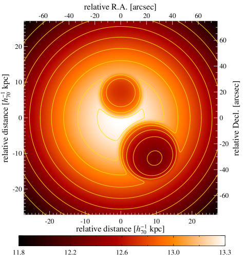
Figure 1: Synthetic ALMA observation of the cool core region of Perseus at the frequency band centered on 144 GHz. Shown is the simulated SZ flux decrement of radio plasma bubbles in units of $\mbox{mJy/arcmin}^{2}$ assuming an ultra-relativistic electron population within the bubbles (scenario 1). The image is smoothed to the resolution of the ALMA compact core configuration ($\mathrm{FWHM}\simeq 2.9\arcsec$). The contour lines have a linear spacing of $0.16\mbox{ mJy/arcmin}^{2}$. For comparison, the size of the ALMA field of view at this frequency is $\mbox{FWHM}_{\mathrm{fov}}\simeq 36\arcsec$.

In this section, only the general setup and the results for the synthetic ALMA observation of the cool core regions of Perseus and Abell 2052 are presented while the interested reader is referred to Appendix A for further details.

To simulate an ALMA observation of the central region of Perseus, we compute the frequency band-averaged SZ flux decrement $\langle\delta I\rangle_{\nu_{0}}$ around the frequency $\nu_{0}=144\mbox{ GHz}$ which samples the extremum of the SZ flux decrement. The resulting simulated SZ flux decrement was convolved with a Gaussian of width $\sigma_{\nu_{0}}\simeq 1.2\arcsec$ to obtain the resolution of this ALMA configuration. Since Perseus has more than 40 degrees of declination and is a Northern object, ALMA will be challenged to observe it, culminating at 25 degrees elevation. However, for a North-South elongated configuration of ALMA about the factor of $(\cos\,65\degr)^{-1}\simeq 2.4$, the beam will be almost round. Assuming an ultra-relativistic electron population within the bubbles yields the SZ flux decrement as shown in Fig. 1 which is similar in morphology to the X-ray image.

To investigate whether the plasma bubbles are detectable in the SZ flux decrement, we define the SZ flux contrast $\rho$:

$$\rho=\frac{I_{\mathrm{A}}-I_{\mathrm{B}}}{I_{\mathrm{A}}+I_{\mathrm{B}}}.$$ (27)

Here, $I_{\mathrm{A}}$ and $I_{\mathrm{B}}$ denote the mean SZ flux decrement of two equally sized solid angle elements within the field of view, one of which measures the SZ flux inside and the other one outside the bubble. Prior information about the angular position of the X-ray cavities allows one to maximize the SZ flux contrast. Adopting Gaussian error propagation and introducing ALMA’s sensitivity in terms of flux density, $\sigma_{\!ALMA}$, yields the signal-to-noise for the $5\sigma$ detection of the bubble:

$$\frac{\mathcal{S}}{\mathcal{N}}\equiv\frac{\rho}{\sigma_{\rho}}=\frac{\sqrt{N_{\mathrm{beam}}}\,\left(I_{\mathrm{A}}^{2}-I_{\mathrm{B}}^{2}\right)}{2\sigma_{\!ALMA}\sqrt{I_{\mathrm{A}}^{2}+I_{\mathrm{B}}^{2}}}\geq 5.$$ (28)

Here, $N_{\mathrm{beam}}$ is the number of statistically independent beams per flux averaged solid angle element (cf. Appendix A). We choose the field of view to be centered on the inner rim of the southern bubble such that equal solid angle elements fall inside and outside the bubble, respectively. The simulated mean SZ flux decrements within the two solid angle elements of the primary beam require only an integration time of 5.1 hours in order to obtain a $5\sigma$ detection of the plasma bubble assuming an ultra-relativistic electron population within the bubble. Uncertainties in the amplitude of the kinetic SZ effect and the geometrical arrangement and shape of the bubbles may slightly modify this result. As a word of caution, this observation time allows a single bubble to be observed in a single pointing while it might be advisable to map the entire central region including both bubbles to get a clearer picture of the structure, and to be convinced that any holes seen in the SZ map at the radio bubbles weren’t just fluctuations also seen elsewhere in the cluster center away from the radio bubbles.

The corresponding observation of Abell 2052 would require an integration time of 38 hours in order to obtain a $5\sigma$ detection of the plasma bubble for the same plasma bubble content, the longer exposures mainly being the result of the higher redshift and the lower central temperature of this cluster.

Table 2: Summary of predicted exposure times for the different combinations of telescopes and clusters. $I_{\mathrm{A}}$ and $I_{\mathrm{B}}$ denote the mean SZ flux decrement of two equally sized solid angle elements within the field of view, one of which measures the SZ flux outside and the other one inside the bubble.

ATelescope: cluster	$I_{A}$	$I_{B}$	exposure
	$[\mbox{mJy amin}^{-2}]$	$[\mbox{mJy amin}^{-2}]$	[hours]
AALMA: Perseus	13.25	12.70	5.1
ALMA: Abell 2052	3.930	3.698	38
GBT: Perseus	11.31	10.85	2.1
GBT: Abell 2052	3.272	3.138	31

5.2 Green Bank Telescope

Green Bank Telescope: Perseus cluster	Green Bank Telescope: Abell 2052

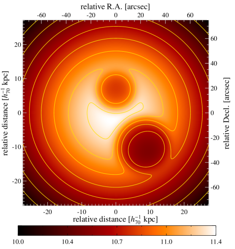
Figure 2: Synthetic GBT observations of the cool core regions of Perseus (left panel) and Abell 2052 (right panel) at the frequency band centered on 90 GHz. Shown is the simulated SZ flux decrement of radio plasma bubbles in units of $\mbox{mJy/arcmin}^{2}$ assuming an ultra-relativistic electron population within the bubbles (scenario 1). The images are smoothed to the resolution the GBT 3 mm receiver ($\mathrm{FWHM}\simeq 8.0\arcsec$). The contour lines have a linear spacing of $0.16\mbox{ mJy/arcmin}^{2}$ (left panel) and $0.08\mbox{ mJy/arcmin}^{2}$ (right panel). For comparison, the size of the GBT field of view at this frequency is $32\arcsec\times 32\arcsec$.

To simulate a GBT observation of the central region of both clusters, we compute the frequency band-averaged SZ flux decrement $\langle\delta I\rangle_{\nu_{0}}$ in the frequency interval $[86\mbox{ GHz},94\mbox{ GHz}]$. The resulting simulated SZ flux decrement was convolved with a Gaussian of width $\sigma\simeq 3.4\arcsec$ to obtain the resolution of the GBT 3 mm receiver. Assuming an ultra-relativistic electron population within the bubbles yields the SZ flux decrement as shown in Fig. 2.

To investigate whether the plasma bubbles are detectable in the SZ flux decrement, we adopt the concept of SZ flux contrast of the previous section. The sensitivity of the upcoming GBT Penn Array Receiver in terms of flux density is given by $\sigma_{\!GBT}=0.25\,(\Delta t)^{-1/2}\mbox{ mJy arcmin}^{-2}$, where $\Delta t$ is the integration time in hours (Mason 2004). We choose the $32\arcsec\times 32\arcsec$ field of view of the GBT to be centered on the inner rim of the southern bubble of Perseus as described above. Assuming an ultra-relativistic electron population within the bubble, we predict a $5\sigma$ detection of the plasma bubble after an integration time of 2.1 hours owing to the better sensitivity of the bolometric receivers on the GBT. This observation time assumes a proper foreground subtraction of the Galactic emission components.

The corresponding observation of Abell 2052 would require an integration time of 31 hours in order to obtain a $5\sigma$ detection of the plasma bubble for the same plasma bubble content. Again, the integration times correspond to a single pointing on the southern bubble while mapping the entire central region would take respectively longer.

6 Composition study of plasma bubbles

In the following, we study exemplarily five physically different scenarios of the composition of the plasma bubble which is as a whole in approximate pressure equilibrium with the ambient ICM. Although these scenarios might not be realized in nature in these pure forms, a realistic SZ flux decrement can be obtained by linearly combining the different scenarios due to the superposition property of the pressure of different populations:

1. The internal pressure is either dominated by CRps, magnetic fields, or ultra-relativistic CRes being characterized by a mean momentum of $\langle p\rangle\gg 1$ in this scenario. This is the most positive case for the detection of the plasma bubbles in the SZ flux decrement, as the bubble volume does not contribute to the SZ flux decrement significantly. Although this is the most positive scenario, it also is the one adopted by most analyses of radio lobes.

2. This scenario assumes the internal pressure to be dominated by a compound of CRp and CRe populations where the latter is described by a power-law distribution:

   $$f_{\mathrm{CRe}}(p,\alpha,p_{1},p_{2})=\frac{(\alpha-1)p^{-\alpha}}{p_{1}^{1-\alpha}-p_{2}^{1-\alpha}}.$$ (29)

   The distribution function is normalized such that its integral over momentum space yields unity. The choice of $p_{1}=1$, $p_{2}=10^{3}$, and $\alpha=2$ implies a mean momentum of $\langle p\rangle\simeq 6.9$ as well as a pseudo-temperature of $k\tilde{T}_{\mathrm{CRe}}\simeq 2.2\,m_{\mathrm{e}}c^{2}\simeq 1.1\mbox{ MeV}$ and represents a plausible scenario for the relativistic composition of the bubble. The CRp and CRe populations each contribute equally to the internal pressure of the bubble representing a remnant plasma originating from the hadronic jet scenario.

3. The dynamically dominant internal pressure support is contributed to equal amounts by relativistic electron and positron populations, respectively. Taking the same parameters for the CRe distribution of the previous scenario, this approach represents the remnant radio plasma originating from the electron-positron jet scenario.

4. A trans-relativistic thermal proton and electron distribution with $kT_{\mathrm{e}}=50\mbox{ keV}$ dominates dynamically over the other non-thermal components:

   $$f_{\mathrm{e,th}}(p,\beta_{\mathrm{th}})=\frac{\beta_{\mathrm{th}}}{K_{2}(\beta_{\mathrm{th}})}p^{2}\exp\left(-\beta_{\mathrm{th}}\sqrt{1+p^{2}}\,\right).$$ (30)

   $K_{2}$ denotes the modified Bessel function of the second kind (Abramowitz & Stegun 1965) which takes care of the proper normalization and $\beta_{\mathrm{th}}=m_{\mathrm{e}}c^{2}/(kT_{\mathrm{e}})$ is the normalized thermal beta-parameter. The mean momentum of this distribution amounts to $\langle p\rangle\simeq 0.55$.

5. This scenario assumes a dynamically dominant hot thermal proton and electron distribution with $kT_{\mathrm{e}}=20\mbox{ keV}$ which exhibits a mean momentum of $\langle p\rangle\simeq 0.33$.

In all cases, the bubble’s sound velocity and thus the barometric scale height are much higher than the corresponding values of the ambient ICM which implies a flat pressure distribution within the plasma bubble. This leads to a reduced internal pressure with respect to the ambient ICM at the inner rim of the bubble and an excess pressure at the outer rim of the bubble, which is responsible for the buoyant rise of the bubble in the cluster atmosphere.

Figure 3: Spectral distortions due to the thermal SZ effect $g(x)$, kinetic SZ effect $h(x)$, relativistic SZ effect due to a population of ultra-relativistic CRes, $\tilde{g}_{\mathrm{UCRe}}=-i(x)\,\tilde{\beta}_{\mathrm{UCRe}}$ (with $p_{1}=3$, $p_{2}=10^{3}$, and $\alpha=2$), relativistic SZ effect due to a population of power-law CRes, $\tilde{g}_{\mathrm{CRe}}=[j(x)-i(x)]\,\tilde{\beta}_{\mathrm{CRe}}$ (with $p_{1}=1$, $p_{2}=10^{3}$, and $\alpha=2$), and the relativistic SZ effect due to a population of trans-relativistic thermal electrons, $\tilde{g}_{\mathrm{50\leavevmode\nobreak\ keV}}=[j(x)-i(x)]\,\beta_{\mathrm{th}}(\mathrm{50\leavevmode\nobreak\ keV})$, as well as due to electrons with $kT_{\mathrm{e}}=20\mbox{ keV}$, respectively.

Figure 3 shows the spectral distortions due to the thermal SZ effect $g(x)$, kinetic SZ effect $h(x)$, and relativistic SZ effect of the various scenarios for the relativistic populations of the bubble composition. The spectral distortions of the relativistic SZ effect are given by $\tilde{g}(x)$ which have been defined in Eqns. (11) through (15). Please note, that the scenarios 2 and 3 exhibit the same spectral distortion $\tilde{g}_{\mathrm{CRe}}$ and that the amplitude of the kinetic SZ effect $w_{\mathrm{gas}}$ is typically one order of magnitude smaller than the amplitude of the thermal SZ effect $y_{\mathrm{gas}}$.

The left panel of Fig. 4 shows the unconvolved SZ flux decrement along an impact parameter through the center of the southern bubble of Perseus at the ALMA frequency band centered on $\nu_{0}=144\mbox{ GHz}$. While the northern bubble of Perseus would evince qualitatively the same behavior, it shows a shallower depth of its SZ cavity due to its smaller geometrical size resulting in a weaker SZ flux contrast (cf. Fig. 1). The depth of the SZ cavity at this frequency range is a measure how relativistic the respective electron population is, i.e. a deeper SZ cavity indicates a higher mean momentum of the electron population. Our studies show a strong signature of the different bubble compositions on the SZ flux decrement. Thus, the combination of X-ray and SZ observations allows one to circumvent the degeneracy between the effects of the bubble composition and of the bubble extent along the line-of-sight on the SZ measurement. This enables us to distinguish a relativistic from a thermal electron population inside the bubble using only a single frequency SZ observation by either a detection or non-detection of the bubble, respectively.

Figure 4: Unconvolved SZ flux decrement along an impact parameter through the center of the southern bubble of Perseus. The left panel shows the SZ flux decrement at the ALMA frequency band centered on $\nu_{0}=144\mbox{ GHz}$ while the right panel assumes a central fiducial frequency of $\nu_{0}\simeq 217\mbox{ GHz}$. Compared are five different scenarios of the composition of the plasma bubbles to the undisturbed SZ profile (dotted thin line), respectively. The three (two) set of lines correspond to three (two) differently assumed average bulk velocities along the line-of-sight, $\bar{\upsilon}_{\mathrm{gas}}$, of the thermal gas of Perseus.

7 Kinetic Sunyaev-Zel’dovich effect

7.1 General considerations

If the cluster is moving towards the observer, the CMB temperature in this direction is increased due to the Doppler effect of the bulk motion of the cluster relative to the rest frame of the CMB (in this case, our convention is such that $\bar{\upsilon}_{\mathrm{gas}}<0$). This enhanced SZ emission implies a reduced SZ flux decrement for frequencies below the crossover frequency of the thermal SZ effect at $\nu_{\mathrm{c}}\simeq 217\mbox{ GHz}$ (for the non-relativistic case). Cosmologically, line-of-sight cluster velocities follow a Gaussian distribution with vanishing mean since the large scale structure is at rest in the comoving CMB-frame and with a standard deviation of $\sigma_{\mathrm{vel}}\simeq 310\mbox{ km s}^{-1}$ as derived from a cosmological structure formation simulation comprising the Hubble volume (Jenkins et al. 2001; Schäfer et al. 2004a).

Theoretically, the turbulent motions of the ICM should also contribute to the kinetic SZ effect. The largest impact is caused by two merging clusters along the line-of-sight which induces a bimodal streaming flow pattern on the sky. However, radio plasma bubbles are mainly observed within cool-core clusters which represent relaxed clusters where the ICM is approximately in hydrostatic equilibrium with the underlying dark matter potential. In this case, only small scale turbulent vortices are expected which exhibit smaller angular momenta. For an isotropic distribution of vortex orientations, line-of-sight integration and beam convolution average the resulting kinetic SZ effect out to zero. Thus, these turbulent motions can only contribute in second order to the thermal SZ effect.

It would be useful to know the peculiar velocity of the galaxy cluster in order to remove the degeneracy of the SZ cavity depth with respect to the different bubble compositions and the kinetic SZ effect. In the case of a general morphology of a galaxy cluster, in particular for non-axis-symmetric objects, it is impossible to unambiguously deproject the cluster in order to derive the peculiar velocity given only a single frequency SZ observation and an X-ray image (Zaroubi et al. 1998, 2001). For multi-frequency SZ observations of the entire cluster, Aghanim et al. (2003) theoretically discuss possibilities in order to break parameter degeneracies between the Compton parameter, the electron temperature and the cluster peculiar velocity for an appropriate choice of observing frequencies. Considering possible gaseous substructure along the line-of-sight towards the radio plasma bubble and a possibly non-spherical bubble geometry, it might be impossible to discriminate between morphologically similar bubble compositions (scenarios 4 and 5) in the case of a single frequency ALMA or GBT observation.

7.2 Perseus plasma bubbles at different frequencies

The left panel of Fig. 4 compares three set of lines corresponding to different average line-of-sight streaming velocities at the ALMA frequency band which samples the extremum of the thermal SZ flux decrement ($\nu_{0}=144\mbox{ GHz}$). The effect of an overall decrease in the SZ flux decrement for the approaching cluster ($\bar{\upsilon}_{\mathrm{gas}}=-300\mbox{ km s}^{-1}$) can be clearly seen. The amplitude of the kinetic SZ effect depends on the dimensionless average velocity of the thermal gas, which amounts in our case to $\bar{\beta}_{\mathrm{gas}}=\bar{\upsilon}_{\mathrm{gas}}/c\simeq 10^{-3}$. On the other hand, the amplitude of the thermal SZ effect depends on the inverse normalized thermal beta-parameter, $\beta_{\mathrm{th}}^{-1}=kT_{\mathrm{e}}/(m_{\mathrm{e}}c^{2})\simeq 10^{-2}$, where we inserted the average temperature of the Perseus cluster. At the extremum of the thermal SZ flux decrement, the kinetic SZ flux amounts to an approximately $10\%$ correction to the thermal SZ effect for the choice of our fiducial cluster velocity. However, this small effect is responsible for the qualitative difference of the observable SZ cavities resulting from plasma bubbles: assuming a receding cluster and a dynamically dominant thermal proton and electron distribution (scenarios 4 and 5), we still obtain a detectable depth of the SZ cavity which almost disappears for an approaching cluster.

The right panel of Fig. 4 shows the unconvolved SZ flux decrement assuming a central frequency of $\nu_{0}=217.34\mbox{ GHz}$ and bandwidth of $\Delta\nu=40\mbox{ GHz}$. Allowing for finite frequency response of the instrument’s receivers, this fiducial frequency corresponds to a vanishing frequency band-averaged thermal SZ flux decrement. Thus, the kinetic SZ effect represents the main effect at this frequency showing a positive SZ flux decrement for a receding cluster, i.e. we would detect a reduced flux of CMB photons in that direction. At this frequency range, a relativistic electron population always causes a positive relativistic SZ flux decrement owing to the higher crossover frequency $\nu_{\mathrm{c}}\gtrsim 217\mbox{ GHz}$ and irrespective of the cluster’s velocity. This effect causes an enhanced SZ flux contrast of the bubble for an approaching cluster compared to a receding one, depending on the specific composition of the plasma bubble.

Most remarkable is the interchange of SZ flux decrements for different bubble compositions compared to the case of $\nu_{0}=144\mbox{ GHz}$. The largest impact of the bubble’s SZ cavity is provided by the trans-relativistic thermal electron population of 50 keV owing to its comparably large frequency band-averaged SZ flux decrement. The SZ flux decrements of the other bubble compositions are smaller because the crossover frequency of the thermal electron population of $kT_{\mathrm{e}}=20\mbox{ keV}$ lies closer to the non-relativistic crossover frequency while the amplitudes of the spectral distortions of the relativistic electron populations are smaller (cf. Fig. 3). Relativistic corrections to the thermal SZ flux resulting from the thermal electrons with temperatures of $kT_{\mathrm{e}}\simeq 3-7\mbox{ keV}$ are negligible: The resulting profiles of the SZ flux decrement are similar in morphology to the kinetic SZ flux decrement and would correspond at this frequency to an additional kinetic SZ effect of only $\sim 10\mbox{ km s}^{-1}$.

Figure 5: Unconvolved SZ flux increment along an impact parameter through the center of the southern bubble of Perseus at the frequency band centered on $\nu_{0}\simeq 470\mbox{ GHz}$. Compared are five different scenarios of the composition of the plasma bubbles to the undisturbed SZ profile (dotted thin line), respectively. The two set of lines correspond to two differently assumed average bulk velocities along the line-of-sight, $\bar{\upsilon}_{\mathrm{gas}}$, of the thermal gas of Perseus.

Owing to the proximity of the Perseus cluster to the Galactic plane, SZ observations at even higher frequencies might be challenging due to the Galactic dust emission which represents the major Galactic foreground at these frequencies (see e.g. Schlegel et al. 1998; Finkbeiner et al. 1999, 2000; Schäfer et al. 2004b). In an exemplary manner, we also show the expected SZ cavity around a fiducial frequency which samples the maximum of the SZ flux increment. For a cluster with a temperature of 5 keV, the normal thermal relativistic corrections disappear at $\nu_{0}=470\mbox{ GHz}$ when taking into account the detector’s finite frequency response of $\Delta\nu=40\mbox{ GHz}$. Secondly, at this frequency the kinetic SZ effect has only a small additional contribution (Aghanim et al. 2003). Hence, one could expect that the SZ signal from the bubble could be even more prominent. This is investigated in Fig. 5 which shows the unconvolved SZ flux increment along an impact parameter through the center of the southern bubble of Perseus at $\nu_{0}=470\mbox{ GHz}$. The different bubble compositions qualitatively show the same behavior as for the SZ decrement at the frequency band around $\nu_{0}=144\mbox{ GHz}$. However, the SZ flux contrast of the bubble is much higher as well as the degeneracy owing to the kinetic SZ effect is reduced. Thus, for clusters not being outshone by the Galactic dust emission, observations at this frequency range seem to be most promising in order to infer the bubble composition.

8 Observing strategy

The previous results imply the following observing strategy for the ALMA compact core configuration or the GBT. A short duration observation (a few hours) of the inner rim of the southern X-ray cavity within the Perseus cool-core region should either yield a $5\sigma$ detection of an SZ cavity or not. The case of a significant detection either proves the existence of a dynamically dominating CRp population, magnetic fields, or an ultra-relativistic CRe population within the radio plasma bubble while the contrary excludes this hypothesis on the $5\sigma$ level.

Such a non-detection of the bubble would require a longer integration time in order to detect the SZ flux decrement of the plasma bubble at the desired significance level. A detection of a very shallow SZ cavity indicates a dynamically dominant hot thermal electron population within radio plasma bubbles. The underlying physical scenario is degenerate for an observed intermediate depth of the SZ cavity (such as an SZ flux level in between our scenarios 3 and 4). Possibilities include trans-relativistic thermal electron distributions or soft CRe power-law distributions exhibiting a spectral index of approximately $\alpha=3$ as well as a small lower cutoff $p_{1}$ implying a mean momentum of $\langle p\rangle\sim 1$. Follow-up multi-frequency SZ observations in combination with X-ray spectroscopy could disentangle the different scenarios and possibly estimate the temperature or spectral characteristics of the dynamically dominating electron population (Shimon & Rephaeli 2002; Enßlin & Hansen 2004). The detection of such an SZ flux would enable one to draw conclusions concerning the particular jet scenario being responsible for the inflation of the plasma bubble.

The case of a deep SZ cavity with an associated detection of dynamically dominating CRps, magnetic fields, or ultra-relativistic CRes leads to an immediate question about the composition of radio ghosts. Thus, an additional SZ observation of the ghost cavity in Perseus could yield answers about the potential entrainment of ICM into the plasma bubble during its buoyant rise in the cluster atmosphere. If a large fraction of entrained gas in the bubble provides significant pressure support, it must have experienced Coulomb heating through CRes in order not to be detected in X-rays. This would result in a reduced SZ flux contrast of the ghost cavity and leads to a faint or undetectable SZ flux decrement of the ghost cavity.

9 Conclusion and outlook

This work provides a theoretical framework for studying the SZ decrement of radio plasma bubbles within clusters of galaxies. X-ray observations are proportional to the square of the thermal electron density and probe the core region of the cluster. On the other hand, the SZ effect is proportional to the thermal electron pressure enabling the detection of plasma bubbles further outwards of the respective clusters. Assuming spherically symmetric plasma bubbles, we simulate an ALMA and a GBT observation of the cool core regions of the Perseus cluster and Abell 2052. In this context, we exemplarily investigate physically different scenarios of the composition of the plasma bubbles: As long as the bubble is dynamically dominated by relativistic electrons, protons, or magnetic fields, there exists a realistic chance to detect plasma bubbles in the SZ flux decrement. Non-detection of radio bubbles with the SZ effect at the position of X-ray cavities hints towards a dynamically dominant hot thermal electron population within radio plasma bubbles. Detection of a non-thermal pressure support should be possible within a few hours observation with ALMA or GBT in the case of Perseus and a few ten hours in the case of Abell 2052.

Pursuing high-sensitivity multi-frequency SZ observations, it will be challenging but not impossible to infer the detailed nature of the different possible populations of the bubble. For realistic observations, the frequency dependence of the relativistic SZ signal is contaminated by the presence of the kinetic SZ signal. It would be optimal to have a frequency channel centered on the crossover frequency of the thermal SZ effect in order to infer the energy spectrum of the dynamically dominating population and to measure the temperature or spectral characteristics of the electron population.

Appendix A Synthetic ALMA observation of the central region of Perseus

This appendix provides additional details of the synthetic ALMA observation of the cool core region of Perseus as well as the expected SZ flux contrast of the southern X-ray cavity. First, we compute the frequency band-averaged SZ flux decrement which is defined by

$$\langle\delta I\rangle_{\nu_{0}}=\frac{\int\mathrm{d}\nu\,\delta I(\nu)R_{\nu_{0}}(\nu)}{\int\mathrm{d}\nu\,R_{\nu_{0}}(\nu)}.$$ (31)

Here, $R_{\nu_{0}}(\nu)$ denotes the frequency response of the ALMA receivers centered on a fiducial frequency $\nu_{0}$ which we assume to be described by a top-hat function:

$$R_{\nu_{0}}(\nu)=\left\{\begin{array}[]{l@{,\:}l}1\hfil,\>&\nu\in\left[\nu_{0}-\Delta\nu/2,\nu_{0}+\Delta\nu/2\right]\\ 0\hfil,\>&\nu\notin\left[\nu_{0}-\Delta\nu/2,\nu_{0}+\Delta\nu/2\right]\end{array}\right.$$ (32)

We choose the ALMA frequency band 4 which samples the extremum of the SZ flux decrement and is characterized by $\nu_{0}=144\mbox{ GHz}$ and $\Delta\nu=38\mbox{ GHz}$ (Brown et al. 2000). The requirement of obtaining the highest flux sensitivity to the largest scales comparable to the field of view at this frequency ($\mbox{FWHM}_{\mathrm{fov}}\simeq 36\arcsec$) calls for the most compact configuration ALMA E with a maximal baseline of $d_{\mathrm{bl}}=150\mbox{ m}$. Thus, we convolve the simulated SZ flux decrement with a Gaussian to obtain the resolution of this configuration, $\mbox{FWHM}\simeq c/(\nu\,d_{\mathrm{bl}})\simeq 2.86\arcsec$. Assuming an ultra-relativistic electron population within the bubbles yields the SZ flux decrement as shown in Fig. 1.

To investigate, whether the plasma bubbles are detectable in the SZ flux decrement, we define the SZ flux contrast $\rho$:

$$\rho=\frac{I_{\mathrm{A}}-I_{\mathrm{B}}}{I_{\mathrm{A}}+I_{\mathrm{B}}}.$$ (33)

Here, $I_{\mathrm{A}}$ and $I_{\mathrm{B}}$ denote the mean SZ flux decrement of two equally sized solid angle elements within the field of view, one of which measures the SZ flux inside and the other one outside the bubble. Adopting Gaussian error propagation and introducing ALMA’s sensitivity per beam in terms of flux density, $\sigma_{\!ALMA}$, yields the uncertainty in $\rho$,

$$\sigma_{\rho} = \sqrt{\left(\frac{\partial\rho}{\partial I_{\mathrm{A}}}\right)^{2}+\left(\frac{\partial\rho}{\partial I_{\mathrm{B}}}\right)^{2}}\,\frac{\sigma_{\!ALMA}}{\sqrt{N_{\mathrm{beam}}}}$$ (34)

$$= \frac{2\sqrt{I_{\mathrm{A}}^{2}+I_{\mathrm{B}}^{2}}}{\left(I_{\mathrm{A}}+I_{\mathrm{B}}\right)^{2}}\,\frac{\sigma_{\!ALMA}}{\sqrt{N_{\mathrm{beam}}}}.$$ (35)

Here, $N_{\mathrm{beam}}=f\,A_{\mathrm{beam}}/(2A_{\mathrm{fov}})$ is the number of statistically independent beams per flux averaged solid angle element, $f\leq 0.5$ measures the fraction of the solid angle of the bubble within the field of view, and the factor of $A_{\mathrm{beam}}/(2A_{\mathrm{fov}})$ accounts for the statistically independent degrees of freedom within the field of view. Combining Eqns. 33 and 35 yields the signal-to-noise for the $5\sigma$ detection of the bubble:

$$\frac{\mathcal{S}}{\mathcal{N}}\equiv\frac{\rho}{\sigma_{\rho}}=\frac{\sqrt{N_{\mathrm{beam}}}\,\left(I_{\mathrm{A}}^{2}-I_{\mathrm{B}}^{2}\right)}{2\sigma_{\!ALMA}\sqrt{I_{\mathrm{A}}^{2}+I_{\mathrm{B}}^{2}}}\geq 5.$$ (36)

The flux density sensitivity $\sigma_{\!ALMA}$ for point sources, which should be approximately applicable in the case of the compact core configuration, is given by Butler et al. (1999):

$$\sigma_{\!ALMA}=\frac{\sqrt{2}\,kT_{\mathrm{sys}}}{\eta\,A_{\mathrm{dish}}\,A_{\mathrm{beam}}\sqrt{\Delta t\,\Delta\nu\,N_{\mathrm{bl}}}}.$$ (37)

Here, $T_{\mathrm{sys}}\simeq 65\mbox{ K}$ denotes the system temperature, $A_{\mathrm{dish}}=\pi D^{2}/4$ the collecting area of each dish ($D=12\mbox{ m}$), $\eta=0.75$ the aperture efficiency, $A_{\mathrm{beam}}=1.13\mbox{ FWHM}^{2}\simeq 9.3\leavevmode\nobreak\ \mathrm{arcsec}^{2}$ the area of the secondary beam, $\Delta t$ the integration time, $\Delta\nu=38\mbox{ GHz}$ the bandwidth, and $N_{\mathrm{bl}}=n(n-1)/2$ the number of baselines, $n=64$ being the number of antennas. We choose the field of view to be centered on the inner rim of the southern bubble such that equal solid angle elements fall inside and outside the bubble, respectively. The simulated mean SZ flux decrements within the two solid angle elements of the primary beam, $I_{\mathrm{A}}=13.25\mbox{ mJy arcmin}^{-2}$ and $I_{\mathrm{B}}=12.70\mbox{ mJy arcmin}^{-2}$, require only an integration time of 5.1 hours in order to obtain a $5\sigma$ detection of the plasma bubble assuming an ultra-relativistic electron population within the bubble. Uncertainties in the amplitude of the kinetic SZ effect and the geometrical arrangement and shape of the bubbles may slightly modify this result.

References

- Abramowitz & Stegun (1965) Abramowitz, M. & Stegun, I. A. 1965, Handbook of mathematical functions (Dover, New York)
- Aghanim et al. (2003) Aghanim, N., Hansen, S. H., Pastor, S., Semikoz, D. V. 2003, Journal of Cosmology and Astro-Particle Physics, 5, 7
- Allen et al. (2001) Allen, S. W., Schmidt, R. W., Fabian, A. C. 2001, MNRAS, 328, L37
- Birkinshaw (1999) Birkinshaw, M. 1999, Phys. Rep, 310, 97
- Blanton et al. (2003) Blanton, E. L., Sarazin, C. L., McNamara, B. R. 2003, ApJ, 585, 227
- Blanton et al. (2001) Blanton, E. L., Sarazin, C. L., McNamara, B. R., Wise, M. W. 2001, ApJ, 558, L15
- Böhringer et al. (1993) Böhringer, H., Voges, W., Fabian, A. C., Edge, A. C., Neumann, D. M. 1993, MNRAS, 264, L25
- Brüggen & Kaiser (2001) Brüggen, M. & Kaiser, C. R. 2001, MNRAS, 325, 676
- Brown et al. (2000) Brown, R., Emerson, D., Baars, J., L., D., et al. 2000, ALMA Project Book, Ch. 2, http://www.eso.org/projects/alma
- Butler et al. (1999) Butler, B., Brown, B., Blitz, L., et al. 1999, ALMA Memo Series No. 243, http://www.eso.org/projects/alma
- Carilli et al. (1994) Carilli, C. L., Perley, R. A., Harris, D. E. 1994, MNRAS, 270, 173
- Celotti et al. (1998) Celotti, A., Kuncic, Z., Rees, M. J., Wardle, J. F. C. 1998, MNRAS, 293, 288
- Churazov et al. (2001) Churazov, E., Brüggen, M., Kaiser, C. R., Böhringer, H., Forman, W. 2001, ApJ, 554, 261
- Churazov et al. (2000) Churazov, E., Forman, W., Jones, C., Böhringer, H. 2000, A&A, 356, 788
- Churazov et al. (2003) Churazov, E., Forman, W., Jones, C., Böhringer, H. 2003, ApJ, 590, 225
- De Young (2003) De Young, D. S. 2003, MNRAS, 343, 719
- Dolgov et al. (2001) Dolgov, A. D., Hansen, S. H., Pastor, S., Semikoz, D. V. 2001, ApJ, 554, 74
- Enßlin (1999) Enßlin, T. A. 1999, in MPE Report, Vol. 271, Diffuse Thermal and Relativistic Plasma in Galaxy Clusters, ed. H. Böhringer, L. Feretti, & P. Schuecker, 275
- Enßlin & Biermann (1998) Enßlin, T. A. & Biermann, P. L. 1998, A&A, 330, 90
- Enßlin & Hansen (2004) Enßlin, T. A. & Hansen, S. H. 2004, astro-ph/0401337
- Enßlin & Heinz (2002) Enßlin, T. A. & Heinz, S. 2002, A&A, 384, L27
- Enßlin & Kaiser (2000) Enßlin, T. A. & Kaiser, C. R. 2000, A&A, 360, 417
- Fabian (2001) Fabian, A. C. 2001, in XXIth Moriond Astrophysics Meeting on ’Galaxy Clusters and the High Redshift Universe Observed in X-rays’, ed. D. M. Neumann
- Fabian et al. (2000) Fabian, A. C., Sanders, J. S., Ettori, S., et al. 2000, MNRAS, 318, L65
- Finkbeiner et al. (1999) Finkbeiner, D. P., Davis, M., Schlegel, D. J. 1999, ApJ, 524, 867
- Finkbeiner et al. (2000) Finkbeiner, D. P., Davis, M., Schlegel, D. J. 2000, ApJ, 544, 81
- Finoguenov & Jones (2001) Finoguenov, A. & Jones, C. 2001, ApJ, 547, L107
- Gull & Northover (1973) Gull, S. F. & Northover, J. E. 1973, Nature, 244, 80
- Hansen et al. (2002) Hansen, S. H., Pastor, S., Semikoz, D. V. 2002, ApJ, 573, L69
- Heinz et al. (2002) Heinz, S., Choi, Y., Reynolds, C. S., Begelman, M. C. 2002, ApJ, 569, L79
- Hirotani et al. (1998) Hirotani, K., Iguchi, S., Kimura, M., Wajima, K. 1998, in Abstracts of the 19th Texas Symposium on Relativistic Astrophysics and Cosmology, held in Paris, France, Dec. 14-18, 1998. Eds.: J. Paul, T. Montmerle, and E. Aubourg (CEA Saclay).
- Huang & Sarazin (1998) Huang, Z. & Sarazin, C. L. 1998, ApJ, 496, 728
- Hudson (2004) Hudson, M. J. 2004, private communication
- Hudson et al. (1997) Hudson, M. J., Lucey, J. R., Smith, R. J., Steel, J. 1997, MNRAS, 291, 488
- Hudson et al. (2004) Hudson, M. J., Smith, R. J., Lucey, J. R., Branchini, E. 2004, MNRAS, 352, 61
- Itoh & Nozawa (2004) Itoh, N. & Nozawa, S. 2004, A&A, 417, 827
- Jenkins et al. (2001) Jenkins, A., Frenk, C. S., White, S. D. M., et al. 2001, MNRAS, 321, 372
- Mason (2004) Mason, B. S. 2004, private communication
- Mazzotta et al. (2002) Mazzotta, P., Kaastra, J. S., Paerels, F. B., et al. 2002, ApJ, 567, L37
- McNamara et al. (2000) McNamara, B. R., Wise, M., Nulsen, P. E. J., et al. 2000, ApJ, 534, L135
- McNamara et al. (2001) McNamara, B. R., Wise, M. W., Nulsen, P. E. J., et al. 2001, ApJ, 562, L149
- Mohr et al. (1999) Mohr, J. J., Mathiesen, B., Evrard, A. E. 1999, ApJ, 517, 627
- Pfrommer & Enßlin (2004) Pfrommer, C. & Enßlin, T. A. 2004, A&A, 413, 17
- Rephaeli (1995a) Rephaeli, Y. 1995a, ARA&A, 33, 541
- Rephaeli (1995b) Rephaeli, Y. 1995b, ApJ, 445, 33
- Sazonov & Sunyaev (2000) Sazonov, S. Y. & Sunyaev, R. A. 2000, A&A, 354, L53
- Schäfer et al. (2004a) Schäfer, B. M., Pfrommer, C., Bartelmann, M., Springel, V., Hernquist, L. 2004a, astro-ph/0407089
- Schäfer et al. (2004b) Schäfer, B. M., Pfrommer, C., Hell, R., Bartelmann, M. 2004b, astro-ph/0407090
- Schindler et al. (2001) Schindler, S., Castillo-Morales, A., De Filippis, E., Schwope, A., Wambsganss, J. 2001, A&A, 376, L27
- Schlegel et al. (1998) Schlegel, D. J., Finkbeiner, D. P., Davis, M. 1998, ApJ, 500, 525
- Shimon & Rephaeli (2002) Shimon, M. & Rephaeli, Y. 2002, ApJ, 575, 12
- Sikora & Madejski (2000) Sikora, M. & Madejski, G. 2000, ApJ, 534, 109
- Sunyaev & Zel’dovich (1972) Sunyaev, R. A. & Zel’dovich, I. B. 1972, Comments Astrophys. Space Phys., 4, 173
- Sunyaev & Zeldovich (1980) Sunyaev, R. A. & Zeldovich, I. B. 1980, ARA&A, 18, 537
- Wright (1979) Wright, E. L. 1979, ApJ, 232, 348
- Zaroubi et al. (2001) Zaroubi, S., Squires, G., de Gasperis, G., et al. 2001, ApJ, 561, 600
- Zaroubi et al. (1998) Zaroubi, S., Squires, G., Hoffman, Y., Silk, J. 1998, ApJ, 500, L87