Constraining Neutrino Masses by CMB Experiments Alone

Abstract

It is shown that a subelectronvolt upper limit can be derived on the neutrino mass from the CMB data alone in the $\Lambda$CDM model with the power-law adiabatic perturbations, without the aid of any other cosmological data. Assuming the flatness of the universe, the constraint we can derive from the current WMAP observations is $\sum m_{\nu}<2.0$ eV at the 95% confidence level for the sum over three species of neutrinos ($m_{\nu}<0.66$ eV for the degenerate neutrinos) by maximising the likelihood over 6 other cosmological parameters. This constraint modifies little even if we abandon the flatness assumption for the spatial curvature. We argue that it would be difficult to improve the limit much beyond $\sum m_{\nu}\lesssim 1.5$ eV using only the CMB data, even if their statistics are substantially improved. However, a significant improvement of the limit is possible if an external input is introduced that constrains the Hubble constant from below. The parameter correlation and the mechanism of CMB perturbations that give rise to the limit on the neutrino mass are also elucidated.

I Introduction

The upper limit on the absolute mass of neutrinos is derived from the end-point spectrum of tritium beta decay experiments. It is not easy, however, to push the limit to the subelectronvolt range. An alternative hope is to resort to cosmological considerations. The presence of massive neutrinos affects cosmic perturbations, most characteristically in a way to reduce the power in the small scale due to free streaming in the early universe. In a low matter density universe the effect is significant even if the neutrino mass is of the order of subelectronvolts Hu:1997mj , and constraints of a few eV as upper limits on the sum mass of three species of neutrinos are obtained from the power of galaxy clustering combined with the normalisation of the fluctuation power at large scales from the magnitude of quadrupole anisotropies in the cosmic microwave background (CMB) temperature field Croft:1999 ; Fukugita:2000 , or from the shape of the power spectrum of galaxy clustering Elgaroey:2002 .

Massive neutrinos also affect perturbations in the CMB temperature field at intermediate to small scales in a less trivial manner (see Ma:1995ey ; Dodelson:1995es for the earlier work). The effect here is via the modification of CMB perturbations, especially through the integrated Sachs-Wolfe effect, rather than simply the reduction of the power at small scales. Combining the CMB multipoles of WMAP with the galaxy clustering data of 2dFGRS, Spergel et al. Spergel:2003cb derived $\sum m_{\nu}<0.7$ eV: using the SDSS power spectrum, Tegmark et al. Tegmark:2003ud give $<1.7$ eV for the sum mass; see also Refs. Elgaroy:2003yh ; Hannestad:2003xv ; Allen:2003pt ; Crotty:2004gm ; Seljak:2004xh . A general problem with the cosmological analyses is how the result depends on explicit or implicit assumptions and systematics, especially when two or more pieces of different types of data, such as CMB multipoles and galaxy clustering data, are combined. In this context it is an important question to ask whether one can derive a comparable limits on the neutrino mass from the CMB data alone. Tegmark et al.’s analysis shows that such a limit is not derived from the CMB data (WMAP data) alone, allowing for the possibility that massive neutrinos represent the entire dark matter at one sigma confidence level, whereas earlier Eisenstein et al.’s work Eisenstein:1998hr seems to forecast the contrary. We consider that this is an important point that deserves further studies, especially in the view that the quality of the CMB temperature field data will be improved in the future, notably by the PLANCK in a half decade time, and it is a consequential question if one can improve the limit on the neutrino mass without resorting to the large-scale galaxy clustering data, for which we always have a suspect for unknown biasing and not well-controlled nonlinear effects.

It is also important to understand whether the limit depends upon the assumption of the exactly flat spatial curvature of the universe, as customarily assumed when the constraints on neutrinos were discussed. We already know that the curvature is quite close to flat, but the possibility of a slight departure from the flatness is not excluded. For instance, the derivation of the consistent Hubble constant from CMB alone depends crucially on the flatness assumption: a slight departure, say by 2% in the spatial curvature, largely modifies the “CMB best value” of the Hubble constant to an unacceptably small value. We see some reason that a small neutrino mass may give an effect similar to non-flat curvature and thus the two effects might cancel, loosening the limit.

In this paper we investigate the problem within the $\Lambda$CDM universe with adiabatic perturbations whether a sensible limit on the neutrino mass can be derived from the CMB data alone, and if this is the case how does the limit depend upon the assumption of the exact flatness of the universe. A particular emphasis is given to elucidating the parameter correlation and the mechanism in the CMB perturbation theory as to how the neutrino mass limit is derived. In our argument we extensively use the “reduced CMB observables”, the position of the first acoustic peak $\ell_{1}$, the height of the first peak normalised to the low $\ell$ value $H_{1}$, the height of the second relative to the first peak $H_{2}$, and the height of the third relative to the first peak $H_{3}$, introduced in Hu et al. Hu:2000ti , and study how the massive neutrinos affect these variables.

We assume that the three neutrinos have a degenerate mass. This will be a realistic assumption if the neutrinos have masses close to the upper limit that concerns us, because the neutrino oscillation experiments tell us that the differences of masses are much smaller than the upper limit. In our numerical work we ignore the tensor perturbations, but we argue that their inclusion would only tighten the limit on the neutrino mass. We assume that the cosmic density perturbations have a power spectrum specified by index $n_{s}$. A small departure from the power spectrum as predicted by slow-roll inflation does not change our analysis. If the departure is at a large amount, such as that indicated by the WMAP team combining their CMB data with the galaxy clustering, our result will need modification: in such a case one cannot argue for the limit on the neutrino mass unless the primordial power spectrum is given.

In the next section, we show with the numerical work that we can derive a sensible limit on the neutrino mass from the CMB data alone under the assumption of the exact spatial flatness of the universe. In Sec. III we consider the effect of massive neutrinos on the reduced CMB observables, and discuss how one can obtain the constraint from the CMB data alone. In Sec. IV we discuss the physics of the response of the reduced CMB observables to massive neutrinos in CMB perturbation theory. In Sec. V, we consider the constraint in non-flat universes, and show that a comparable constraint is derived. The conclusion is given in Sec. VI.

II Limit on the neutrino mass from WMAP alone

Figure 1: Minimum $\chi^{2}$ as a function of the neutrino energy density $\omega_{\nu}$. The solid curve is for the flat universe. The dotted and the dashed curves show the cases for a negative and a positive curvature universe, respectively.

$\omega_{\nu}$	$\omega_{b}$	$\omega_{m}$	$h$	$\tau$	$n_{s}$	$A$	$\chi^{2}$	$\ell_{1}$	$H_{1}$	$H_{2}$	$H_{3}$
0.00	0.0230	0.145	0.689	0.116	0.973	1133.1	1428.6	220	6.68	0.449	0.456
0.001	0.0231	0.145	0.682	0.116	0.973	1119.1	1428.7	220	6.70	0.449	0.459
0.01	0.0224	0.145	0.600	0.105	0.950	1044.7	1428.8	219	6.60	0.447	0.452
0.02	0.0218	0.137	0.564	0.0936	0.918	1096.7	1431.0	219	6.33	0.442	0.432
0.025	0.0216	0.130	0.556	0.0901	0.904	1137.0	1433.0	219	6.21	0.441	0.422
0.03	0.0219	0.128	0.551	0.0835	0.894	1155.7	1435.2	219	6.12	0.439	0.417
0.04	0.0223	0.120	0.545	0.0793	0.883	1188.9	1439.4	220	6.02	0.438	0.411
0.05	0.0230	0.112	0.545	0.0794	0.876	1215.4	1442.7	220	5.95	0.437	0.408
0.06	0.0237	0.104	0.545	0.0788	0.873	1228.1	1444.9	220	5.92	0.437	0.406
0.08	0.0250	0.0864	0.547	0.0694	0.867	1230.5	1447.1	220	5.90	0.437	0.402
0.10	0.0260	0.0686	0.547	0.0696	0.868	1226.2	1447.6	221	5.90	0.440	0.401
0.12	0.0270	0.0496	0.548	0.0720	0.869	1226.2	1447.3	221	5.92	0.441	0.399
0.14	0.0278	0.0310	0.548	0.0741	0.874	1213.0	1446.7	221	5.95	0.443	0.401

Table 1: Solutions for $\chi^{2}_{\rm min}(\omega_{\nu})$.

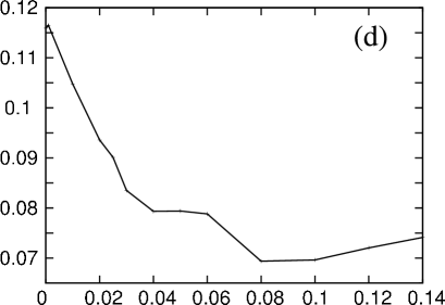
Figure 2: The cosmological parameters for the solutions that give minimum $\chi^{2}$ as a function of $\omega_{\nu}$. The two line segmants shown in panel (c) are the cases for a negative (dotted line) and a positive (dashed line) curvature universe.

Figure 3: The values of reduced CMB observables for the solutions that give minimum $\chi^{2}$ as a function of $\omega_{\nu}$.

The parameters of the $\Lambda$CDM model we shall consider are the baryon density $\omega_{b}\equiv\Omega_{b}h^{2}$, the matter density $\omega_{m}\equiv\Omega_{m}h^{2}$ (which includes baryons but excludes neutrinos), the Hubble constant $h$, the reionisation optical depth $\tau$, the scalar spectral index $n_{s}$ of the power-law adiabatic perturbations, and overall normalization $A$, where $\Omega_{i}$ denotes the energy density in units of the critical density and $h$ is $H_{0}=100\ h\ {\rm km}\ {\rm s}^{-1}{\rm Mpc}^{-1}$. We ignore the tensor perturbations. We define the normalisation parameter by $A=\ell(\ell+1)C^{TT}_{\ell}/2\pi$ in units of $\mu$K² at $\ell=2$, which differs from the WMAP definition. In addition, we include the neutrino mass density $\omega_{\nu}\equiv\Omega_{\nu}h^{2}$, which is related to the neutrino mass as

$$\omega_{\nu}=\frac{\Sigma m_{\nu}}{94.1\ {\rm eV}}\ .$$ (1)

We assume three generations of neutrinos with their masses being degenerate, $m_{\nu_{e}}=m_{\nu_{\mu}}=m_{\nu_{\tau}}$, so $m_{\nu}=31.4\ \omega_{\nu}$ eV. The vacuum energy is taken to satisfy the flat curvature $\Omega_{\rm tot}\equiv\Omega_{\Lambda}+\Omega_{m}+\Omega_{\nu}=1$, but this condition is relaxed in Sec. V. We often write $\omega_{\Lambda}\equiv\Omega_{\Lambda}h^{2}$. We run CMBFAST Seljak:1996is to calculate CMB multipoles for the total of $1\times 10^{6}$ sets of parameters in the course of our work. The $\chi^{2}$ are computed for the entire temperature (TT) and polarisation (TE) data set of WMAP (899 and 449 points, respectively) using the likelihood code supplied by the WMAP team Verde:2003ey ; Hinshaw:2003ex ; Kogut:2003et .

We search for the $\chi^{2}$ minimum for fixed $\omega_{\nu}$, and refer to the resulting $\chi^{2}$ minimum for a fixed $\omega_{\nu}$ as $\chi^{2}_{\rm min}(\omega_{\nu})$. We prefer to use a deterministic search for the minimum rather than the Markov chain Monte Carlo (MCMC) method that is popular in the recent work for the CMB analysis, since we find that the latter, while it is in principle efficient to find a gross global structure of the likelihood function, often fails to yield the accurate shape of the likelihood function away from the minimum unless the chain is long.

To search for the $\chi^{2}$ minimum in 6 parameter ($\omega_{b}$, $\omega_{m}$, $h$, $\tau$, $n_{s}$, $A$) space, we adopt a nested grid search. Technically, we apply the Brent method brent of the successive parabolic interpolation to find a minimum with respect to one specific parameter with other parameters at a given grid, and successively apply this method to remaining parameters to find the global minimum. We describe more details of this minimisation procedure in Appendix A. If more than one conspicuous $\chi^{2}$ minima are detected in the process, we apply this method to each local minimum. We run the CMBFAST code typically $10^{5}$ times to find the global minimum for a given $\omega_{\nu}$. Note that the adoption of the Brent method greatly reduces the number of grids needed for a required accuracy.

In order to obtain the likelihood function with respect to a specifc parameter, we must in principle integrate over the parameters other than the one that concerns us. The $\chi^{2}$ function could be different significantly from the true likelihood function, if the distribution is not Gaussian. To verify this point, we carry out an adaptive Monte Carlo integral using the Vegas code lepage to check if the likelihood function inferred from the $\chi^{2}$ function differs significantly from that obtained by integarting over parameter space. The integral is performed for the cases of $\omega_{\nu}=0$ and 0.08, the latter being the value with which Tegmark et al. give a rather high likelihood. In particular, we want to check if a local minimum that gives a relatively large $\chi^{2}$ is favoured from a large measure of parameter space. In so far as we have examined, there is no evidence that the likelihood inferred from $\chi^{2}$ function differs significantly from that obtained from the integral (examples are shown below). In particular, we do not find the case where the integration measure overcomes an excess $\chi^{2}$: the parameter sets that give the global $\chi^{2}$ minimum always represent the maximally likely parameters in the case we studied.

	$\omega_{b}$	$\omega_{m}$	$h$	$\tau$	$n_{s}$	$\chi^{2}_{min}$
Ours	0.0230	0.145	0.689	0.116	0.973	1428.6
Spergel et al. Spergel:2003cb	0.024$\pm$0.001	0.14$\pm$0.02	0.72$\pm$0.05	$0.166^{+0.076}_{-0.071}$	0.99$\pm$ 0.04	1431
Tegmark et al. Tegmark:2003ud	$0.0245^{+0.0050}_{-0.0019}$	$0.140^{+0.020}_{-0.018}$	$0.74^{+0.18}_{-0.07}$	$0.21^{+0.24}_{-0.11}$	$1.02^{+0.16}_{-0.06}$	1431.5

Table 2: Comparison of the solution for the massless neutrino with those given by Spergel et al. and Tegmark et al. The errors stand for one $\sigma$ confidence level.

$\omega_{b}$	$\omega_{m}$	$h$	$\tau$	$n_{s}$	$A$	$\chi^{2}$	$\ell_{1}$	$H_{1}$	$H_{2}$	$H_{3}$	remarks
0.0230	0.145	0.689	0.116	0.973	1133.1	1428.6	220	6.68	0.449	0.456	global mininum
0.0305	0.121	0.957	0.487	1.21	1428.1	1428.8	221	6.31	0.453	0.481	local minimum

Table 3: Parameters for the two $\chi^{2}$ minima for $\omega_{\nu}=0$.

The solutions that give a $\chi^{2}$ minimum for a given $\omega_{\nu}$ are presented in Table 1. The $\chi^{2}_{\rm min}$ as a function of the neutrino mass density is shown in Figure 1, and the 6 parameters of the solution for each neutrino mass density, also given in the table, are displayed in Figure 2. The corresponding four reduced CMB observables (defined below) are shown in Figure 3 for the use in the next section.

We first note that the 6 parameters for $\omega_{\nu}=0$ agree with those of the comparable solutions of Spergel et al. Spergel:2003cb and Tegmark et al. Tegmark:2003ud within one sigma errors (see Table 2), verifying that our minimisation to find the global minimum works at least as good as the MCMC method they used. In fact, the overall $\chi^{2}$ we attained is appreciably smaller than the two authors’ for the same set of input data ($\chi^{2}_{\rm spergel}-\chi^{2}_{\rm ours}=2.4$, and $\chi^{2}_{\rm tegmark}-\chi^{2}_{\rm ours}=2.9$). We may ascribe this to a finer grid of the parameters close to the minimum in our work. We find bimodal structure of the $\chi^{2}$ surface, most clearly visible for $n_{s}$ and $\tau$ that are strongly correlated to each other Tegmark:2003ud . The two minima are found at $n_{s}=0.973$ and $n_{s}=1.21$ with the second minimum having a slightly larger $\chi^{2}$, $\chi^{2}(n_{s}=1.21)-\chi^{2}(n_{s}=0.973)=0.2$, or the relative likelihood of 1.1: see Table 3. The two parameter sets are disjoint by a hill with a height more than one $\sigma$. The Vegas integration over multiparameter space centred on the two extrema indicates that the former minimum is favoured over the latter by the ratio of 1.3 in terms of the likelihood value. That is, likelihood from the $\chi^{2}$ estimator is a good approximation to the ‘true’ value obtained by marginalising the parameters, i.e., even in this case where the distribution is deviated from Gaussian the $\chi^{2}$ function is likely a reasonable approximation of the likelihood function. Furthermore, we observed that the one-parameter distributions with respect to the other five parameters are close to Gaussian once we require $n_{s}$ to be around the peak at $n_{s}=0.973$ (see Appendix B). This suggests that the distribution in multidimensional space is likely not far from the Gaussian. Hence, we infer that the $\chi^{2}$ statistics well approximates the reality.

The bimodal structure we find is consistent with what was found by Tegmark et al., but our likelihood of the second minimum is much higher than that reported (the ratio of likelihoods between the two extrema by Tegmark et al. is 2.5). We suspect that Markov chain of Tegmark et al. does not sample well around the second minimum. This point is demonstrated in more detail in Appendix B. This is an example that the current application of the MCMC does not give an accurate likelihood function away from the global minimum. Of course, the second solution is an unphysical one in the sense that it is allowed only at the cost of an unacceptably high reionisation optical depth ($\tau\approx 0.5$); the solution is deleted with some prior on $\tau$. The resulting parameters $\omega_{b}$, and $h$ are also deviated significantly from the values derived from other observations.

In Figure 1 we observe that $\chi^{2}_{\rm min}(\omega_{\nu})$ increases with the neutrino mass density. The curve of $\chi^{2}$ minimum is close to a parabola except in the immediate vicinity of $\omega_{\nu}=0$. Taking $\Delta\chi^{2}\equiv\chi^{2}_{\rm min}(\omega_{\nu})-\chi^{2}_{\rm min}=4$ to set an upper limit on $\omega_{\nu}$ at the 95% confidence level, we obtain

$$\omega_{\nu}<0.024,\hskip 14.22636pt{\rm or}\hskip 14.22636ptm_{\nu}<0.75\ {\rm eV}.$$ (2)

Since the likelihood function with respect to $n_{s}$ and $\omega_{\nu}$, ${\cal L}=\exp[-\Delta\chi^{2}(n_{s},\omega_{\nu})/2]$, which is constructed by minimising the five other parameters, is visibly deviated from Gaussian, we integrated it over $n_{s}$ and then over $\omega_{\nu}$. This yields the 95% confidence limit

$$\omega_{\nu}<0.021,\hskip 14.22636pt{\rm or}\hskip 14.22636ptm_{\nu}<0.66\ {\rm eV},$$ (3)

which is close to Eq. (2), a simple reading from $\chi^{2}$. [The difference primarily comes from the second peak of the $\chi^{2}$ function, which is ignored in Eq. (2)]. If the distributions of the five other parameters are close to Gaussian, a two-dimensional integral is sufficient to obtain an accurate likelihood.

We cannot compare this limit on the neutrino mass directly with those derived in Spergel et al. and Tegmark et al. Tegmark:2003ud , in which those authors used the galaxy clustering data as additional inputs. On the other hand, the latter authors claim that WMAP alone does not give a limit on the neutrino mass and that the massive neutrinos can make up 100% of dark matter at about one $\sigma$ confidence unless galaxy clustering data are used. Our result contradicts this. We do not find a parameter set that gives acceptable $\chi^{2}$ for the neutrino mass density beyond the limit. Furthermore, the measure of the parameter space does not seem to increase for a larger $\omega_{\nu}$. Our Vegas integrals give a relative likelihood between $\omega_{\nu}=0$ and $\omega_{\nu}=0.08$ to be $7\times 10^{-5}$, which is consistent with the estimate from our $\chi^{2}$ curve $5\times 10^{-5}$, whereas Tegmark et al.’s value is 0.6. We suspect that sampling of the Markov chain of Tegmark et al. does not give an accurate likelihood function away from $m_{\nu}=0$ that is the global minimum, as similarly happened with the case of $n_{s}$ discussed above and in Appendix B. In particular, we do not find a mixed-dark-matter-model ($\Omega_{m}+\Omega_{\nu}=1$) like solution: the CMB multipoles of the hot dark matter model with some sets of parameters are visibly similar to the observation Elgaroy:2003yh , but a closer inspection shows that $\chi^{2}$ is always unacceptably large, given a high accuracy of the WMAP data. In the following section we see a reason how can one obtain the limit on the neutrino mass density from the CMB data alone.

We remark that the current WMAP TE data do not seem to play a significant role in deriving our limit, as we find in separate runs of the $\chi^{2}$ minimisation using only the TT data: the $\chi^{2}$ curves differ little between the two cases. This somewhat differs from the forecast of Eisenstein et al.Eisenstein:1998hr who indicated a tighter error allowance that would result with the WMAP polarisation data.

As a final remark, the two $\chi^{2}$ minima found for $\omega_{\nu}=0$ persist up to $\omega_{\nu}\sim 0.04$, but the one that corresponds to the “unphysical solution” disappears for $\omega_{\nu}\gtrsim 0.05$.

III The reduced CMB observables and the neutrino mass

III.1 The reduced CMB observables and the goodness of the $\Lambda$CDM fit

Following Ref. Hu:2000ti , we focus on four quantities which characterise the shape of the CMB spectrum: the position of the first peak $\ell_{1}$, the height of the first peak relative to the large angular-scale amplitude evaluated at $\ell=10$,

$$H_{1}\equiv\left(\frac{\Delta T_{l_{1}}}{\Delta T_{10}}\right)^{2},$$ (4)

the ratio of the second peak height to the first,

$$H_{2}\equiv\left(\frac{\Delta T_{l_{2}}}{\Delta T_{l_{1}}}\right)^{2},$$ (5)

and the ratio of the third peak height to the first,

$$H_{3}\equiv\left(\frac{\Delta T_{l_{3}}}{\Delta T_{l_{1}}}\right)^{2},$$ (6)

where $(\Delta T_{l})^{2}\equiv l(l+1)C^{TT}_{l}/2\pi$ and $C^{TT}_{l}$ is the multipole coefficient of the temperature anisotropy.

Taking the advantage that we generated one million CMB templets, we estimate the reduced CMB observables from the envelope drawn by the entire set of the templets. Our sampling is dense enough to define the correct envelope at least for small $\Delta\chi^{2}$ that concerns us. The result is

$$\ell_{1} = 220^{+1.5}_{-1},$$ (7)

$$H_{1} = 6.7^{+0.3}_{-0.6},$$ (8)

$$H_{2} = 0.449\pm 0.007,$$ (9)

$$H_{3} = 0.46^{+0.04}_{-0.02},$$ (10)

which is shown in Figure 4. The error is 1 standard deviation obtained by halving the range that gives 2 $\sigma$ error, i.e., $\Delta\chi^{2}\equiv\chi^{2}-\chi^{2}_{\rm min}=4$, because the structure of the $\chi^{2}$ curve is not always parabolic at around $\Delta\chi^{2}\approx 1$. The central values are the best fit solution given in Table 1. Eqs. (9) and (10) are consistent with the values Tegmark et al. Tegmark:2003ud quoted for their best parameter set ($H_{1}$ is not given). We note particularly small errors for $\ell_{1}$ and $H_{2}$, which play an important role in the argument given in the next subsection. In addition, we draw the envelopes for the case of a few non-zero neutrino masses. They give increasingly larger $\chi^{2}$ as the mass increases, in particular for $\omega_{\nu}\geq 0.02$; the widths of the $\chi^{2}$ valleys become somewhat narrowed as $\omega_{\nu}$ increases.

We also attempt to obtain the four reduced CMB observables from the fits that give a $\chi^{2}$ minimum for a restricted range of $\ell$ using our CMB templets, as was done in Hu:2000ti . We calculate $\chi^{2}$ using the TT data of appropriate multipole ranges. We use $75\leq l\leq 375$ for $\ell_{1}$, $7\leq l\leq 375$ for $H_{1}$, $75\leq l\leq 375$ and $450\leq l\leq 600$ for $H_{2}$, and $75\leq l\leq 375$ and $750\leq l\leq 875$ for $H_{3}$. The results are displayed in Figure 4 above. We obtain

$$\ell_{1} = [~{}219,~{}222~{}],$$ (11)

$$H_{1} = [~{}6.5,~{}7.9~{}],$$ (12)

$$H_{2} = [~{}0.430,~{}0.452~{}],$$ (13)

$$H_{3} = [~{}0.362,~{}0.488~{}].$$ (14)

The numbers bracketed are the 1 $\sigma$ range obtained by halving the 2 $\sigma$ range of the $\chi^{2}_{\rm local}$ curve. An inspection of the fits of the templets to the obeserved CMB multipoles indicates that the data are well represented by those templets. Figure 4 may give the impression that the $\chi^{2}$ curves do not agree with those obtained from the envelope of the global $\Lambda$CDM fit: the valley of the $\chi^{2}$ curves is generally wider, and the positions of the bottom of valley is somewhat shifted; the $\chi^{2}_{\rm local}$ of the best global fit solution is larger than the best local fits by $\Delta\chi^{2}\approx 2$. The central values of Eqs. (7) to (10), however, fall in the one $\sigma$ range of Eqs. (11) to (14). Our analysis, showing that the best global fit and the local fits resulted in the consistent reduced CMB parameters within 1 $\sigma$, leads us to conclude the goodness of the $\Lambda$CDM fit.

For the consideration given in the next subsection, where we are concerned with the problem how much massive neutrinos increase $\chi^{2}$ for the CMB data relative to the $\omega_{\nu}=0$ solution, we should use Eqs. (11) - (14), rather than Eqs. (7) - (10), which are obtained by restricted parameter searches.

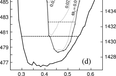
Figure 4: Constraints on the four reduced CMB observables. Local $\chi^{2}$ is computed using restricted sets of multipoles as explained in the text and is measured with $\chi^{2}_{\rm local}$ in the relevant range indicated in the left ordinate. The $\chi^{2}$ of global solution is measured for the value with respect to the entire data set as measured in the right ordinate. The relative normalisation is fixed so that the global solution that gives $\chi^{2}$ minimum gives the local $\chi^{2}$ value measured in the left ordinate. Dotted curves are the envelopes for $\omega_{\nu}=0.01$, 0.02 and 0.03 in the order of increasing minimum $\chi^{2}$. The horizontal dashed line segments show the position of $\chi^{2}-\chi^{2}_{\rm min}=4$.

III.2 Reduced CMB observables and the neutrino mass

We calculate the response of the observables $O_{i}=\ell_{1}$, $H_{1}$ $H_{2}$ and $H_{3}$ with respect to the variation of cosmological parameters $x_{j}$, i.e., the partial derivatives $\partial O_{i}/\partial x_{j}$, around the global best fit, following Ref. Hu:2000ti . We vary the parameters typically by $\pm$50% with a step of 5% and take the difference from the reference values. We find that the responses are quite linear against the amount of the variations of the 6 parameters. The exception is the response to the neutrino density parameter, for which it is shown separately. The resulting partial derivatives are:

$$\Delta\ell_{1} = 16\frac{\Delta\omega_{b}}{\omega_{b}}-25\frac{\Delta\omega_{m}}{\omega_{m}}-47\frac{\Delta h}{h}+36\frac{\Delta n_{s}}{n_{s}}+f_{\Delta\ell_{1}}(\omega_{\nu}),$$ (15)

$$\Delta H_{1} = 3.0\frac{\Delta\omega_{b}}{\omega_{b}}-3.0\frac{\Delta\omega_{m}}{\omega_{m}}-2.2\frac{\Delta h}{h}-1.7\frac{\Delta\tau}{\tau}+18\frac{\Delta n_{s}}{n_{s}}+f_{\Delta H_{1}}(\omega_{\nu}),$$ (16)

$$\Delta H_{2} = -0.30\frac{\Delta\omega_{b}}{\omega_{b}}+0.015\frac{\Delta\omega_{m}}{\omega_{m}}+0.41\frac{\Delta n_{s}}{n_{s}}+f_{\Delta H_{2}}(\omega_{\nu}),$$ (17)

$$\Delta H_{3} = -0.19\frac{\Delta\omega_{b}}{\omega_{b}}+0.21\frac{\Delta\omega_{m}}{\omega_{m}}+0.56\frac{\Delta n_{s}}{n_{s}}+f_{\Delta H_{3}}(\omega_{\nu}).$$ (18)

Here $\Omega_{\rm tot}=1$ is kept fixed, and $f_{\Delta O_{i}}(\omega_{\nu})$ stands for the variation with respect to the neutrino mass density. The responses of $H_{2}$ and $H_{3}$ to $h$, and those of $\ell_{1}$, $H_{2}$ and $H_{3}$ to $\tau$ are small, so they are omitted in the expressions. Page et al. Page:2003fa , evaluated the partial derivatives for $H_{2}$ and $H_{3}$ to the variations of $\omega_{b}$, $\omega_{m}$ and $n_{s}$ for the WMAP data using the analytic expressions Hu:2000ti . Our empirical derivatives for these quantities are consistent with their analytic evaluation.

Figure 5: Response of the four reduced CMB observables to the variation of $\omega_{\nu}$. The isolated points show the values at $\omega_{\nu}=0$, which do not connect to the $\omega_{\nu}\neq 0$ values smoothly.

We draw the response of $O_{i}$ against the variation of $\omega_{\nu}$ for the range $\omega_{\nu}=0$ to 0.04 in Figures. 5. Note that an increase in $\omega_{\nu}$ accompanies a decrease in $\Omega_{\Lambda}$ as we keep $\Omega_{\rm tot}=1$ and $\omega_{m}=\omega_{\rm cdm}+\omega_{b}$ fixed. We see small glitches from $\omega_{\nu}=0$ to the neighbouring point in Figures. 5 (b), (c) and (d). This is probably a numerical artefact caused by the implementation of the massive neutrino subroutine in the CMBFAST code, and we ignore these glitches since they are much smaller than the errors of the CMB data.

We observe that the response of the four observables against $\omega_{\nu}$ changes at around $\omega_{\nu}\approx 0.015$. As $\omega_{\nu}$ increases beyond it, the decrease of $\ell_{1}$ becomes gentle; the $H_{1}$, which increases with $\omega_{\nu}$ up to $\omega_{\nu}=0.017$, turns to decrease. $H_{2}$ and $H_{3}$ change little ($<0.5$%) between $\omega_{\nu}=0$ and 0.015, but then begin to increase. We can understand this turning point as the competition between neutrino free streaming and recombination. Neutrinos become non-relativistic before the recombination when $\omega_{\nu}\gtrsim 0.017$ and they become non-relativistic after the recombination when $\omega_{\nu}\lesssim 0.017$. We can show that the behaviours, at least for $\ell_{1}$ and $H_{1}$, are quantitatively understood by simple analytical considerations, but let us defer this problem to the next section.

Here, we are concerned with the problem how the constraint on the neutrino mass is obtained from the CMB data alone, given observational and empirical information of $\ell_{1}$, $H_{1}$, $H_{2}$ and $H_{3}$. We argue that we cannot derive a constraint for $\omega_{\nu}<0.017$ but an upper limit likely exists at some neutrino mass in the region $\omega_{\nu}\gtrsim 0.02$.

We first consider $\omega_{\nu}<0.017$. In this regime, as seen in Figure 5, $\ell_{1}$ decreases and $H_{1}$ increases while $H_{2}$ and $H_{3}$ change little with increasing $\omega_{\nu}$. The change induced by $\omega_{\nu}$ in $\ell_{1}$ is significant, but according to Eq. (15) it is cancelled to a large degree by a decrease of $h$ [Fig. 2 (c)], as seen in Figure 3 (a). For $\omega_{\nu}=0.015$, say, we need $h$ to decrease from 0.69 to 0.58, but this change is harmless. The decrease of $h$, however, causes an increase of $H_{1}$ (see (16)) in addition to the direct increase due to $\omega_{\nu}$. The increase of $H_{1}$ is cancelled by decreases of $n_{s}$ and $\omega_{b}$, whereas those two decreases tend to cancel in $H_{2}$ and $H_{3}$. The error allowance of $H_{1}$ is large enough that a good cancellation is not required, and hence it is easy to make the induced changes of $H_{2}$ and $H_{3}$ cancelled to within their error allowances. The large error of $H_{1}$ arises primarily from the cosmic scatter, $\sigma\sim\sqrt{2/(2\ell+1)}$, in small $\ell$ modes (which we estimate to give $\delta H_{1}\approx\pm 0.5$); so it seems unlikely that it will be reduced greatly in data expected in the future. Therefore, unless external observational data are introduced we cannot derive a constraint on the neutrino mass density for $\omega_{\nu}$ substantially smaller than 0.017, consistent with the flat $\chi^{2}$ dependence around $\omega_{\nu}=0$ in Figure 1. This will remain to be true even if the quality of the CMB data is improved.

When $\omega_{\nu}>0.017$, massive neutrinos contribute to increase $H_{2}$ and $H_{3}$ as seen in Figures. 5(c) and (d) in addition to a further decrease of $\ell_{1}$. Looking at Eq. (17) and Eq. (18), the increase in $H_{2}$ and $H_{3}$ due to massive neutrinos may be compensated by either increasing $\omega_{b}$ or decreasing $n_{s}$. Actually, as shown in Figure 2 (a) and (e), the decrease of $n_{s}$ occurs to minimise $\chi^{2}$. This is owing to a steeper increase of $H_{3}$ than $H_{2}$ with the increase of $\omega_{\nu}$: $\Delta H_{3}/\Delta\omega_{\nu}>\Delta H_{2}/\Delta\omega_{\nu}$ in Figure. 5 (c) and (d). Such increases are more efficiently compensated by the decrease of $n_{s}$ than by the increase of $\omega_{b}$, as read from Eqs. (17) and (18), which indicate that $\Delta H_{3}/\Delta n_{s}>\Delta H_{2}/\Delta n_{s}$ whereas $|\Delta H_{3}/\Delta\omega_{b}|<|\Delta H_{2}/\Delta\omega_{b}|$. [NB: $\omega_{b}(\omega_{\nu}=0.017)-\omega_{b}(\omega_{\nu}=0)$ is negative for the reason discussed in the above paragraph, but turns to increasing for $\omega_{\nu}>0.017$ to collaborate in the requirement.] In other words, massive neutrinos enhance the multipoles more on smaller scales (larger $\ell$), which causes an effect similar to the increase of $n_{s}$ than the decrease of $\omega_{b}$, which increases even peaks more strongly.

In passing, it is worth noting that $\omega_{\nu}$ and $n_{s}$ are negatively correlated in this argument, in contrast to the naive expectation of the positive correlation from the effect of massive neutrinos that diminish the small scale power. The latter implies that the limit on the neutrino mass loosens for increasing $n_{s}$ (e.g., Fukugita:2000 ). The CMB argument works in the opposite way.

The cancellation of the effect due to $\omega_{\nu}$ in the acoustic peaks by decreasing $n_{s}$ increases the large-scale amplitude significantly, as is manifest in a large coefficient of $\Delta n_{s}/n_{s}$ in Eq. (16). With a tight error allowance for $H_{2}$ the decrease of $n_{s}$ compels $H_{1}$ to decrease largely, as seen in Figure 3 (b), and to push down $H_{1}$ below the allowed error range ($H_{1}\geq 6.2$ at 1.5 $\sigma$) at around $\omega_{\nu}\sim 0.02$, while $H_{2}$ and $H_{3}$ stay within the boundary of errors given in Eqs. (13) and (14). This corresponds to the upper limit of $\omega_{\nu}$ we obtained, i.e., $\omega_{\nu}<0.021$ (at 95%), in a numerical study of the $\chi^{2}$ test.

Let us visit briefly the possibility of varying $\tau$ to increase $H_{1}$. From Eq. (16), a large decrease of $\tau$ would make it increase without disrupting $\ell_{1}$, $H_{2}$ and $H_{3}$. However, $\tau$ can not be reduced as much as one wants, as displayed in Figure 2 (d). The observed high amplitude at the lowest multipoles of the TE mode needs a non-negligible amount of the reionization optical depth.

We may also ask whether the inclusion of the tensor perturbations change the limit. Hu et al. Hu:2000ti give

$$\Delta H_{1}\approx-5\frac{r_{t}}{1+0.76r_{t}}$$ (19)

where $r_{t}=1.4[\Delta T_{10}^{(T)}/\Delta T_{10}^{(S)}]^{2}$ is the tensor to scalar ratio at $\ell=10$. This means that the inclusion of the tensor mode collaborates to lower $H_{1}$, and thus only tightens the limit on the neutrino mass density.

These considerations show that one can derive the limit on the neutrino mass density of the order of $\omega_{\nu}\sim 0.02$ from WMAP data alone. They also show that the limit may be improved to $\omega_{\nu}\sim 0.017$ with the use of improved CMB data, but it would not be easy to go beyond. Even with the extremely high precision data anticipated from PLANCK, the limit we expect will be $\omega_{\nu}<0.013$ at the 95% confidence level: the increase of $\chi^{2}$ is very slow for $\omega_{\nu}\lesssim 0.01$.

The efficient way to improve the limit on $\omega_{\nu}$ is to introduce observations that constrain the Hubble constant, either directly or indirectly, from below. This is because the most prominent effect caused by light neutrino is to change the position of the first peak and it is absorbed into a lowering shift of the Hubble constant. Should one require that $H_{0}>65$ km s^-1Mpc^-1, a significantly stronger limit of the order of $\omega_{\nu}\lesssim 0.01$ would be derived even with the current CMB data.

IV Analytic considerations on the effect of massive neutrinos

IV.1 The position of the first peak

Here, we attempt to understand the effect of massive neutrinos on the reduced CMB observables. We may take the epoch when the neutrino of mass $m_{\nu}$ becomes nonrelativistic as its momentum $p_{\nu}\sim m_{\nu}$, i.e., $T_{\nu,\rm nr}=m_{\nu}/3$. The corresponding redshift is

$$1+z_{\rm nr} = \frac{T_{\nu,\rm nr}}{T_{\nu,0}}$$ (20)

$$= 1.99\times 10^{3}(m_{\nu}/{\rm eV})$$ (21)

$$= 6.24\times 10^{4}\omega_{\nu},$$ (22)

where $\sum m_{\nu}=3m_{\nu}$ is used for the last equality. This is compared with the redshift at recombination $z_{\rm rec}=1088$ Spergel:2003cb , which is insensitive to the mass of neutrinos. Neutrinos become non-relativistic before recombination, i.e., $z_{\rm nr}>z_{\rm rec}$, if

$$\omega_{\nu}\gtrsim 0.017,$$ (23)

but otherwise they remain relativistic and freely stream till post recombination epochs. This $\omega_{\nu}$ corresponds approximately to the turning points of the curves of $\ell_{1}$, $H_{1}$, $H_{2}$ and $H_{3}$ observed in Figure 5.

We denote the energy density in the form $\omega\equiv\Omega h^{2}=\rho h^{2}/\rho_{\rm cr,0}$, where the critical density $\rho_{\rm cr,0}=3M_{\rm pl}H^{2}_{0}$ with the Planck mass defined by the gravity scale $M_{\rm pl}^{2}=1/8\pi G$, and the subscript $0$ expresses values at the present epoch. The matter and photon energy densities are

$$\rho_{m}(a)h^{2}/\rho_{\rm cr,0}=\omega_{m,0}\left(\frac{a}{a_{0}}\right)^{-3},\hskip 14.22636pt\rho_{\gamma}(a)h^{2}/\rho_{\rm cr,0}=\omega_{\gamma,0}\left(\frac{a}{a_{0}}\right)^{-4},$$ (24)

where the present photon energy density $\omega_{\gamma,0}=2.48\times 10^{-5}$ for $T_{\gamma,0}=2.725$ K Mather:1998gm . The neutrino energy density is

$$\rho_{\nu}(a)h^{2}/\rho_{\rm cr,0} = \frac{45}{\pi^{4}}\left(\frac{4}{11}\right)^{4/3}\omega_{\gamma,0}\left(\frac{a}{a_{0}}\right)^{-4}\int_{0}^{\infty}\sqrt{x^{2}+y^{2}}x^{2}(e^{x}+1)^{-1}dx,$$ (25)

where

$$y=m_{\nu}(11/4)^{1/3}(a/a_{0})T_{\gamma,0}^{-1},$$ (26)

and $x$ is the normalised momentum variable and three flavours of neutrinos are assumed to have a degenerate mass. The vacuum energy is

$$\rho_{\Lambda}(a)h^{2}/\rho_{\rm cr,0} = \omega_{\Lambda,0}$$ (27)

$$= h^{2}-\omega_{m,0}-\omega_{\nu,0},$$ (28)

for the flat universe. The total energy density is $\rho_{\rm tot}=\rho_{m}+\rho_{\gamma}+\rho_{\nu}+\rho_{\Lambda}$. With $\rho_{\rm tot}$, the cosmic expansion rate $H=\dot{a}/a$ is given by $H^{2}=\rho_{\rm tot}/3M_{\rm pl}^{2}$, which is used to evaluate the conformal time $\eta$,

$$\eta(a)=\int\frac{dt}{a}=\int_{0}^{a}\frac{da^{\prime}}{a^{\prime 2}H}\ .$$ (29)

The position of the $m$-th peak $\ell_{m}$ is determined from that of the acoustic peak $\ell_{A}$ and the phase shift $\phi_{m}$, which depends weakly on $m$ Hu:2000ti ,

$$\ell_{m}=\ell_{A}(m-\phi_{m}),$$ (30)

where the acoustic scale is defined by

$$\ell_{A}=\pi\frac{r_{\theta}(\eta_{\rm rec})}{r_{s}(\eta_{\rm rec})},$$ (31)

with $r_{s}(\eta_{\rm rec})$ the sound horizon at the recombination epoch and $r_{\theta}(\eta_{\rm rec})$ is the comoving angular diameter distance to the last scattering surface, $r_{\theta}(\eta_{\rm rec})=\eta_{0}-\eta_{\rm rec}$ in the flat universe. The sound horizon is given by

$$r_{s}(a)\equiv\int_{0}^{\eta(a)}c_{s}d\eta=\int_{0}^{a}c_{s}(a^{\prime})\frac{da^{\prime}}{a^{\prime 2}H},$$ (32)

where the sound speed $c_{s}^{2}=(1/3)(1+R)^{-1}$ with $R=3\rho_{b}/4\rho_{\gamma}=3a\omega_{b,0}/4\omega_{\gamma,0}$. The $c_{s}$ depends only on photons and baryons, and the effect of neutrino masses enters into the sound horizon only through the modification of the expansion law. The phase shift in Eq. (30) arises from the decay of gravitational potential due to radiation growth suppression when the universe is not fully matter dominated, which later modifies the gravitational redshift that the photons would otherwise suffer from the Sachs-Wolfe effect Hu:1994jd . This is sometimes called the early integrated Sachs-Wolfe effect. The evaluation of the integral gives $\ell_{A}\sim 300$, which is considerably larger than the physical position of $\ell_{1}$: the difference is ascribed to the phase shift $\phi_{1}$, which is estimated in what follows.

The enhancement of the amplitude for scales between the first acoustic peak and the horizon crossing at the matter domination due to the early integrated Sachs-Wolfe effect makes the first peak formed at a scale larger than the acoustic peak. An accurate evaluation of the phase shift $\phi$ requires the full solution of the coupled Boltzmann equations. Instead, we use the fitting formula given in Ref. Hu:2000ti ,

$$\phi_{1}\approx 0.267\left(\frac{r_{\rm rec}}{0.3}\right)^{0.1},$$ (33)

where $r_{\rm rec}$ is the radiation-to-matter energy ratio $r\equiv\rho_{r}/\rho_{m}$ at the recombination. The appearance of the radiation-to-matter energy ratio as the prime variable is motivated by the physics of the integrated Sachs-Wolfe effect Hu:1994jd . Precisely speaking, this fitting formula is given for massless neutrinos, but it is expected to be valid for massive case provided that $r_{\rm rec}$ is modified appropriately, because the effect of massive neutrinos on the integrated Sachs-Wolfe effect is primarily through the change of $r_{\rm rec}$. A larger radiation-to-matter energy ratio leads to a larger enhancement and hence a larger phase shift as indicated by Eq. (33). Massive neutrinos with $\omega_{\nu}\gtrsim 0.017$ act in a way to suppress this effect.

The ratio $r_{\rm rec}$ in the presence of massive neutrinos is calculated as follows. We take neutrinos that have momentum larger than $m_{\nu}$ as radiation, and those having smaller momentum as matter. Accordingly, we split $\rho_{\nu}$ into the radiation component $\rho_{\nu,r}$ and the matter component $\rho_{\nu,m}$, as

$$\rho_{\nu,r}(a)h^{2}/\rho_{\rm cr,0} = \frac{45}{\pi^{4}}\left(\frac{4}{11}\right)^{4/3}\omega_{\gamma,0}\left(\frac{a}{a_{0}}\right)^{-4}\int_{y}^{\infty}\sqrt{x^{2}+y^{2}}x^{2}(e^{x}+1)^{-1}dx,$$ (34)

$$\rho_{\nu,m}(a)h^{2}/\rho_{\rm cr,0} = \frac{45}{\pi^{4}}\left(\frac{4}{11}\right)^{4/3}\omega_{\gamma,0}\left(\frac{a}{a_{0}}\right)^{-4}\int_{0}^{y}\sqrt{x^{2}+y^{2}}x^{2}(e^{x}+1)^{-1}dx,$$ (35)

by dividing the integration range at the value in Eq. (26). The radiation-to-matter energy ratio is calculated as

$$\xi=(\rho_{\gamma}+\rho_{\nu,r})/(\rho_{m}+\rho_{\nu,m}),$$ (36)

which is used to compute $\phi_{1}$ in Eq. (33).

The first peak position thus calculated as a function of $\omega_{\nu}$ is shown in Figure 6 together with the curve from the full numerical computation presented earlier. The agreement is excellent, validating the prescription described here. For a reference we also draw the case where the phase shift is fixed at the zero-neutrino-mass value, $(1-\phi_{1})\sim 220/300$. This curve agrees with the accurate result for small neutrino masses, but starts deviating from $\omega_{\nu}\approx 0.015$, i.e., when neutrinos become nonrelativistic before the recombination epoch. This stands for the error that we count neutrinos as radiation even when they are non-relativistic at the recombination, and hence, overestimates the early integrated Sachs-Wolfe effect, so does the phase shift $\phi_{1}$. This consideration demonstrates that the change of the slope in $\ell_{1}$ at $\omega_{\nu}\approx 0.017$ is a result of the reduction of the early integrated Sachs-Wolfe effect by the neutrinos that become nonrelativistic before the recombination epoch.

Figure 6: Dependence of $\ell_{1}$ on $\omega_{\nu}$ calculated from Eq. (30) (dashed line), as compared with the accurate numerical solution (solid line). The dotted line shows the case when the effect of massive neutrinos on the early Sachs-Wolfe effect is ignored.

IV.2 Hights of the acoustic peaks

It is known that free-streaming of massive neutrinos causes a larger decay in the gravitational potential $\Phi$. This drives the acoustic oscillation of the baryon-photon fluid more strongly, so that the amplitude of temperature anisotropies within the free-streaming scale is enhanced through the monopole term $\Theta_{0}+\Psi$ in the harmonic expansion of the temperature perturbations Dodelson:1995es . The conformal time corresponding to the free-streaming scale is calculated as $\eta_{\rm nr}=\eta(a_{\rm nr})$ where $a_{\rm nr}$ is known from Eq. (22). This is the distance over which relativistic neutrinos move freely. The multipole $\ell_{\rm nr}$ corresponding to this scale is Hu:1994jd :

$$\ell_{\rm nr} \simeq \frac{2\pi r_{\theta}(\eta_{\rm rec})}{\eta_{\rm nr}},$$ (37)

which we show in Figure 7 for $\omega_{m,0}=0.14$ and $h=0.69$, and $z_{\rm rec}=1088$. The multipole amplitudes for $\ell>\ell_{\rm nr}$ are affected by free streaming. For $\omega_{\nu}>0.017$, the amplitude on the scale $\ell>300$ is enhanced Dodelson:1995es . This means that only the second and higher peaks receive the effect.

Figure 7: Multipoles corresponding to the neutrino free-streaming scale.

The first peak receives little the effect of the decay of gravitational potential, and the variation of $H_{1}$ with $\omega_{\nu}$ is understood by a simple consideration. The gentle increase of $H_{1}$ for $\omega_{\nu}\lesssim 0.017$ is understood by the decrease of $\Omega_{\Lambda}$ to compensate the neutrino energy density in the flat universe and an associated decrease of the integrated Sachs-Wolfe effect from the late domination of $\Lambda$, which enhances $C_{10}$. The effect continues to the region $\omega_{\nu}\gtrsim 0.017$, but in this regime massive neutrinos act as the nonrelativistic dark matter at recombination and the effect from the increase of the amount of matter overcomes; hence $H_{1}$ begins to decrease [$\Delta H_{1}/\Delta\omega_{m}<0$ as seen in Eq. (16)]. This indicates that $\omega_{\nu}\sim 0.017$ is again the turning point, as we saw in Figure 5. In what follows we verify this reasoning by a more quantitative argument.

Our strategy is to reduce the theory with massive neutrinos to an effective, mock theory without massive neutrinos, for which we have an established understanding Hu:1994jd ; Hu:2000ti . If neutrinos are light they are taken as radiation, and if heavy, they are regarded as matter. For $\omega_{\nu}\approx 0.017$, they contribute as both matter and radiation, and are handled by splitting the neutrino energy density into the radiation and matter parts as in Eqs. (34) and (35). We count the matter part of neutrinos at the recombination as additional “CDM”. We then have the effective matter density,

$${\tilde{\omega}}_{m}=\omega_{m,0}+\frac{\rho_{\nu,m}(a_{\rm rec})}{\rho_{\nu,r}(a_{\rm rec})+\rho_{\nu,m}(a_{\rm rec})}\omega_{\nu,0},$$ (38)

where $a_{\rm rec}=1/1089$; see Figure 8 (a).

In order to mimic the true matter-radiation equality epoch in the theory without having massive neutrinos, we try to vary the effective number of neutrino species $N_{\nu}$. This ensures nearly the same amount of the early integrated Sachs-Wolfe effect generated in the massless neutrino world. The scale factor at the equality $a_{\rm eq}$ as a function of $\omega_{\nu}$ is calculated from the condition $\xi(a_{\rm eq})=1$ where $\xi$ is defined by Eq. (36). The result is shown in Figure 8 (b) . From the conventional calculation giving $1+z_{\rm eq}=a_{\rm eq}^{-1}=80950\omega_{m}/(2+0.454N_{\nu})$ for $\omega_{\nu}=0$, the effective $N_{\nu}$ we want is

$$N_{\nu}=\frac{80950{\tilde{\omega}}_{m}a_{\rm eq}(\omega_{\nu,0})-2}{0.454},$$ (39)

which is shown in Figure 8 (c).

We also want to adjust $\Omega_{\Lambda}$ so that the integrated Sachs-Wolfe effect in the $\Lambda$ dominated epoch would be the same in the two universes. Noting that the CMB perturbation depends on $h$ in the form $\Omega h^{2}$, this may be accomplished by shifting $h$. Because the flat universe requires $(\omega_{m}+\omega_{\nu,0})h^{-2}+\Omega_{\Lambda}=1$ for the massive neutrino case, and $\omega_{m}\tilde{h}^{-2}+\Omega_{\Lambda}=1$ for the massless case, $h$ has to be reduced as

$$\tilde{h}=h\sqrt{\frac{\omega_{m}}{\omega_{m}+\omega_{\nu,0}}}.$$ (40)

We consider that the massless neutrino theory with these parameter shifts captures the main features of the theory with massive neutrinos, at least for the first acoustic peak. In fact, as shown in Figure 9, this mock theory reproduces very well the full calculation of $H_{1}$ with massive neutrinos. In the same figure, we also show the two curves calculated by adjusting either $\omega_{m}$ and $N_{\nu}$ alone or $h$ alone, which represents, respectively, the effect of massive neutrinos as matter or the increase of the vacuum energy. The former curve is flat for $\omega_{\nu}\lesssim 0.017$ and turns down henceforth. These component curves demonstrate how $H_{1}$ is built.

Figure 8: Effective parameters of the massless neutrino theory that are required to mock the massless neutrino world.

Figure 9: Dependence of $H_{1}$ on $\omega_{\nu}$ predicted in the mock massless neutrino theory (dashed line), as compared with the true theory with massive neutrinos (solid line). For illustration, the results with the theories, where only the early integrated Sachs-Wolfe effect is mocked by changing $\omega_{m}$ and $N_{\nu}$ (dotted line) and only the late Sachs-Wolfe effect is mocked by changing $h$, are also shown (dot-dashed line).

Figure 10: Dependence of (a) $H_{2}$ and (b) $H_{3}$ on $\omega_{\nu}$ predicted in the mock massless neutrino theory (dashed line), as compared with the true theory with massive neutrinos (solid line).

The second and third peaks are enhanced by free streaming of massive neutrinos Dodelson:1995es . Ignoring this effect, however, we plot $H_{2}$ and $H_{3}$ in Figure 10 for the mock theory we used to reproduce $H_{1}$. Obviously, they do not give the correct dependence for massive neutrinos, underestimating the true values of the changes in $H_{2}$ and $H_{3}$ for $\omega_{\nu}\gtrsim 0.017$. The effect of the potential decay is more prominent in $H_{2}$ (Figure 10 (a)) to which the contribution of CDM is small but the baryon is the major contributor (see Eq. 17). The increase of $H_{3}$ is partly accounted for by the modification of the $\omega_{m}$ term that enters into $H_{3}$ in Eq. (18). Dodelson et al. Dodelson:1995es showed that the increase of the second and third peaks is understood by the potential decay. We do not pursue our analysis further, as it would not give us more insight than that given by Dodelson et al.’s analysis.

V The neutrino mass constraint in non-flat universes

We remove the assumption of $\Omega_{\rm tot}=1$ and study the constraint on the neutrino mass in positive and negative curvature universes. We made a $\chi^{2}$ minimum search only for a few values of $\omega_{\nu}$ close to the upper limit obtained in the flat universe, since the search is time-consuming but an upper limit comparable to the one for the flat universe is anticipated from an analytic argument. We only consider the universe with $\Omega_{\rm tot}=1.02$, 1.04 (positive curvature) and $\Omega_{\rm tot}=0.98$ (negative curvature), which are still allowed from WMAP. The solutions that give a $\chi^{2}$ minimum are given for $\omega_{\nu}=0$, 0.02, 0.025 and 0.03 in Table 4 for the positive curvature case ($\Omega_{\rm tot}=1.02$) and in Table 5 for the negative curvature case. The minimum $\chi^{2}$ is plotted in Figure 1 presented earlier. The figure shows that the $\chi^{2}_{\rm min}$ are slightly smaller for the positive curvature and larger for the negative curvature for a given $\omega_{\nu}(\neq 0)$. We find, however, that this does not change the limit on the neutrino mass. For $\omega_{\nu}=0$, the universe of a slightly positive curvature is somewhat more favoured, viz. $\chi^{2}({\rm flat},\omega_{\nu}=0)-\chi^{2}(\Omega_{\rm tot}=1.02,\omega_{\nu}=0)=1$, as already known in earlier analyses Spergel:2003cb ; Tegmark:2003ud . This decrease of $\chi^{2}$ at the global minimum compensates the decrease of $\chi^{2}$ seen at $\omega_{\nu}\approx 0.02$. So, when the likelihood is computed relative to the global minimum in parameter space allowing $\Omega_{\rm tot}$ to vary, the limit on the neutrino mass remains unchanged. We also find that the introduction of massive neutrinos always increases $\chi^{2}$ relative to the case of massless neutrinos; the presence of massive neutrinos do not modify the limit on the curvature. We finally note that the limit on massive neutrinos becomes tightened when $\Omega_{\rm tot}\gtrsim 1.03$.

$\omega_{\nu}$	$\omega_{b}$	$\omega_{m}$	$h$	$\tau$	$n_{s}$	$A$	$\chi^{2}$	$\ell_{1}$	$H_{1}$	$H_{2}$	$H_{3}$
0.00	0.0230	0.145	0.608	0.1222	0.973	1048.5	1427.6	220	6.92	0.448	0.454
0.02	0.0214	0.133	0.515	0.0873	0.910	1098.9	1430.4	219	6.40	0.443	0.424
0.025	0.0217	0.133	0.504	0.0878	0.905	1119.9	1432.4	219	6.31	0.440	0.423
0.03	0.0217	0.126	0.501	0.0865	0.890	1173.2	1434.6	219	6.16	0.438	0.413

Table 4: Solutions for $\chi^{2}_{\rm min}(\omega_{\nu})$ in the positive curvature universe with $\Omega_{{\rm tot}}=1.02$.

$\omega_{\nu}$	$\omega_{b}$	$\omega_{m}$	$h$	$\tau$	$n_{s}$	$A$	$\chi^{2}$	$\ell_{1}$	$H_{1}$	$H_{2}$	$H_{3}$
0.02	0.0220	0.139	0.640	0.0878	0.923	1127.1	1431.5	219	6.23	0.442	0.435
0.025	0.0220	0.134	0.627	0.0871	0.912	1146.9	1433.5	219	6.15	0.440	0.428
0.03	0.0220	0.129	0.624	0.0790	0.900	1171.4	1435.7	219	6.06	0.439	0.420

Table 5: Solutions for $\chi^{2}_{\rm min}(\omega_{\nu})$ in the negative curvature universe with $\Omega_{{\rm tot}}=0.98$.

It is easy to see how the effect of massive neutrinos is modified from the case of the flat universe. We first note that the partial derivatives with respect to $\Omega_{\rm tot}$

$$\Delta\ell_{1} = -360\frac{\Delta\Omega_{\rm tot}}{\Omega_{\rm tot}},$$ (41)

$$\Delta H_{1} = +4.5\frac{\Delta\Omega_{\rm tot}}{\Omega_{\rm tot}}.$$ (42)

The first relation shows the well-known dependence on $\Omega_{\rm tot}$ that the last scattering surface is magnified in the positive curvature universe. The second relation arises from the late integrated Sachs-Wolfe effect. For $\Omega_{\rm tot}>1$ the reduction of the late integrated Sachs-Wolfe effect decreases $C_{10}$, and hence increases $H_{1}$. $H_{2}$ and $H_{3}$ do not depend on $\Omega_{\rm tot}$. At a first glance one might suspect that a large response of $\ell_{1}$ to $\Omega_{\rm tot}$ for $\Omega_{\rm tot}<1$ would cancel the negative change of $\ell_{1}$ induced by a finite neutrino mass and relax the limit for the negative curvature universe. This, however, is not the case.

The position of $\ell_{1}$ is tightly constrained by the data. So the change in $\ell_{1}$ from either the massive neutrino or the departure from the flat space curvature is compensated by the change in $h$ that is unconstrained. The negative curvature makes this shift smaller, and the positive makes it larger as seen in Figure 2 (c). Note that among the 6 cosmological parameters, only $h$ receives a significant change when a small curvature is introduced. All other parameters change no more than a few percent from the values for the flat universe. The positive curvature increases $H_{1}$ via Eq. (42) and an extra decrease of $h$ also increases $H_{1}$. The increase of $H_{1}$ makes some more allowance to the observational lower limit of $H_{1}$, which lowers $\chi^{2}$ and would in principle weakens the constraint. However, when we remove the spatial flatness assumption, the global $\chi^{2}$ minimum, realised at $\omega_{\nu}=0$, occurs at a $\chi^{2}$ smaller than that for the flat universe. This offsets the decrease of $\chi^{2}(\omega_{\nu}\neq 0)$, and we obtain the limit on the neutrino mass virtually unchanged from the case for the flat universe.

Although the limit on the neutrino mass is formally unchanged in a positive curvature universe, the cost is a significant decrease of $h$ as seen in Figure 2 (c). To realise the 2 $\sigma$ limit, $\omega_{\nu}\sim 0.021$, we are led to $H_{0}\approx 50$ km s^-1Mpc^-1, an unacceptably small value.

The argument may go in the opposite way for the negative curvature, but the limit on the neutrino mass becomes substantially stronger. We calculate $\Delta\chi^{2}$ in a full non-zero curvature parameter space: for negative curvatures $\Delta\chi^{2}(\omega_{\nu}=0)$ is already significant relative to the global minimum that is realised in a positive curvature universe.

Note that our discussion does not deal with $H_{2}$ and $H_{3}$, because these quantities depend on neither $\Omega_{\rm tot}$ or $h$ directly. The change of these quantities takes place only through the adjustment of other parameters, and is small.

In conclusion we find that the constraint on the neutrino mass we obtained for the flat universe $\omega_{\nu}<0.021$ is unchanged even when a non-zero spatial curvature is allowed.

VI Conclusion

We showed that the subelectronvolt upper limit can be derived on the neutrino mass from the CMB data alone within the $\Lambda$CDM model with adiabatic perturbations. This is contrary to the statements made in Elgarøy and Lahav Elgaroy:2003yh and Tegmark et al.Tegmark:2003ud , who stressed that the large-scale galaxy clustering information is essential to derive the limit on the neutrino mass. Assuming the flatness of the universe, the constraint we obtained from the one-year data of the WMAP observation alone by maximising the likelihood is $\omega_{\nu}<0.021$ or $\sum m_{\nu}<2.0$ eV at the 95% confidence level (for the degenerate neutrinos, which are close to the reality if the neutrino mass is close to the limit, $m_{\nu}<0.66$ eV). This is slightly weaker than the limit $<1.7$ eV Tegmark:2003ud derived by the combined use of WMAP and SDSS data, or similar limits that are obtained by combining more different types of data Spergel:2003cb ; Elgaroy:2003yh ; Hannestad:2003xv ; Allen:2003pt ; Crotty:2004gm ; Seljak:2004xh , but our limit is a robust result in the sense that it does not receive any systematics from biasing, non-linear effects and others, and solely determined by the CMB data for which systematics are controlled very well. Our constraint is unchanged even if we relax the flatness assumption. The inclusion of the tensor perturbation only tightens the limit. The assumption we still need is the power-law primordial fluctuation spectrum.

We argued that it would not be easy to improve the limit beyond $\sum m_{\nu}\lesssim 1.5$ eV using the CMB data alone, even if the CMB multipole data are substantially improved. This “critical limit” corresponds to the situation when neutrino becomes nonrelativistic at recombination epoch. That is, we can derive the constraint when neutrinos become nonrelativistic before the recombination epoch. The improvement of the limit on the neutrino mass requires some external inputs, most characteristically the lower limit on the Hubble constant, or those that effectively leads to the constraint on the Hubble constant, such as the Type Ia supernova Hubble diagram or the large-scale clustering of galaxies. If $H_{0}$ would receives a firm lower limit, say $H_{0}>65$ km s^-1Mpc^-1, the upper limit on the neutrino mass would be tightened to $\sum m_{\nu}<0.8$ eV.

We demonstrated the mechanism as to how these constraints are derived, using the reduced CMB observables, $\ell_{1}$, $H_{1}$, $H_{2}$ and $H_{3}$ introduced by Hu:2000ti , and studying their responses to the neutrino mass density. The key point is that $\ell_{1}$ and $H_{2}$ are constrained to narrow ranges by observation, and the variation of the cosmological parameters induced by the finite neutrino density cannot be accommodated in the error budget of $H_{1}$ with the increase of the neutrino mass beyond $\sum m_{\nu}\sim 2$ eV.

We also showed that the response of the reduced CMB observables, in particular $\ell_{1}$ and $H_{1}$, to the neutrino mass density is understood by the modification of the integrated Sachs-Wolfe effect in the presence of massive neutrinos. In addition, free streaming of massive neutrinos promotes the decay of gravitational potential that enhances $H_{2}$ and $H_{3}$, whose scales are within free streaming Dodelson:1995es . This leads to the negative correlation between $n_{s}$ and $m_{\nu}$, in contrast to the positive correlation expected from the suppression of the small scale power due to massive neutrinos.

The most important message from our analysis is that (i) one can derive the upper limit on the neutrino mass, which is only slightly weaker than is quoted in the modern literature, using the CMB (WMAP) data alone: hereby, one can avoid to make use of the mixed data of different quality or with possible systematic effects such as biasing and nonlinear effects for galaxies, and (ii) one may improve the limit by a modest amount even when the quality of the CMB data is improved, but not much. For a substantial improvement of the limit one needs a constraint on the Hubble constant from below.

Appendix A Multidimensional $\chi^{2}$-minimization

Our problem is to minimise $f=\chi^{2}(n_{s},\omega_{m},\omega_{b},\tau,h,A)$ in 6-dimensional parameter space. Since we want to avoid to calculate the derivative, we adopt the Brent method brent and generalise it to a multidimensional problem. For one dimensional problem the Brent method samples 3 points, $f(x_{a}),f(x_{c}),f(x_{b})$, and draw a parabola that connects the three $f$’s to find the value $x_{1}$ that give the valley of $f$. Then $f(x_{1})$ and the two neighbouring $f$’s are used to find the next parabola and its valley at $x_{2}$. This process is successively applied until desired convergence.

For multidimensional problem, say, $f(x,y,z)$, we first minimise $f$ with respect to $z$, by applying the Brent method in this direction, with $x$ and $y$ fixed to an arbitrary grid $x_{a}$ and $y_{a}$. We find successively new $z$ grids $z_{1}(x_{a},y_{a})$, $z_{2}(x_{a},y_{a})$, …, and eventually reach $f(x_{a},y_{a},z_{\rm min}(x_{a},y_{a}))$. We next minimise it with respect to $y$ using $(y_{a},y_{b},y_{c})$. We carry out the $z$ minimisation for $y_{b}$ and $y_{c}$, i.e., $f(x_{a},y_{b},z_{\rm min}(x_{a},y_{b}))$ and $f(x_{a},y_{c},z_{\rm min}(x_{a},y_{c}))$, and successively adding a new $y$ grid, $y_{1},y_{2}...$, while repeating the $z$ minimisation procedure at each step; we eventually arrive at $f(x_{a},y_{\rm min}(x_{a}),z_{\rm min}(x_{a},y_{\rm min}(x_{a})))$. We repeat the same procedure with respect to $x$. Starting from

$$f(x_{a},y_{\rm min}(x_{a}),z_{\rm min}(x_{a},y_{\rm min}(x_{a}))),$$

$$f(x_{b},y_{\rm min}(x_{b}),z_{\rm min}(x_{b},y_{\rm min}(x_{b}))),$$

$$f(x_{c},y_{\rm min}(x_{c}),z_{\rm min}(x_{c},y_{\rm min}(x_{c}))),$$

we finally find

$$f(x_{\rm min},y_{\rm min}(x_{\rm min}),z_{\rm min}(x_{\rm min},y_{\rm min}(x_{\rm min}))),$$

which is the desired result.

For our problem of $f=\chi^{2}(n_{s},\omega_{m},\omega_{b},\tau,h,A)$, applying the minimisation in the order of $A,h,\tau,\omega_{b},\omega_{m}$ and $n_{s}$, the final value would be $\chi^{2}(n_{s,\rm min},\omega_{m,\rm min},\omega_{b,\rm min},\tau_{\rm min},h_{\rm min},A_{\rm min})$, where the omitted arguments are

$$\omega_{m,\rm min} = \omega_{m,\rm min}(n_{s,\rm min}),$$ (43)

$$\omega_{b,\rm min} = \omega_{b,\rm min}(n_{s,\rm min},\omega_{m,\rm min}),$$ (44)

$$\tau_{\rm min} = \tau_{\rm min}(n_{s,\rm min},\omega_{m,\rm min},\omega_{b,\rm min}),$$ (45)

$$h_{\rm min} = h_{\rm min}(n_{s,\rm min},\omega_{m,\rm min},\omega_{b,\rm min},\tau_{\rm min}),$$ (46)

$$A_{\rm min} = A_{\rm min}(n_{s,\rm min},\omega_{m,\rm min},\omega_{b,\rm min},\tau_{\rm min},h_{\rm min}).$$ (47)

We find that this nested one-dimensional minimizations works well for the WMAP $\chi^{2}$ function and the minimum obtained gives $\chi^{2}$ lower than those found by the Markov chain Monte Carlo methods given in the literature. A caution is needed for the outermost nest, the minimization with respect to $n_{s}$. We find two minima for a small $\omega_{\nu}$. So we apply the minimisation procedure for each case separately. If more than one mininum is found in the course of intermediate minimisation, we must divide the parameter space and the minimisation procedure must be applied separately. We do not find, however, such cases other than that quoted above.

Appendix B Comparison of the grid search and MCMC

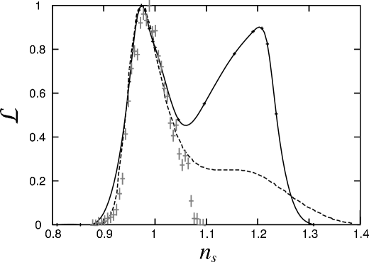
Figure 11: Likelihood functions ($\omega_{\nu}=0$) for $n_{s}$ estimated from our $\chi^{2}$ statistics (solid line), as compared with those from MCMC given by the WMAP group (data points with errors) and Tegmark et al. (dashed line). The maximum is normalised to unity.

Figure 12: An example of the likelihood function for $\omega_{m}$ with $n_{s}$ fixed to 0.98 and $\omega_{\nu}$ to zero. The 10 data points are fitted with a Gaussian function. The maximum is normalised to unity.

We compare the likelihood function for $\omega_{\nu}=0$ inferred from the $\chi^{2}$ function with those obtained by the MCMC given in the literature. In Figure 11 we present ${\cal L}=\exp(-\Delta\chi^{2}/2)$ and $\cal L$ given by Tegmark et al. Tegmark:2003ud and Spergel et al. Spergel:2003cb for the variable $n_{s}$. We see that our likelihood function agrees very well with Tegmark et al.’s for $n_{s}<1.05$, but it starts deviating for $n_{s}>1.05$, where our likelihood function is much larger, meaning that Tegmark et al.’s chain does not find a true local minimum near the second peak. We emphasise that the relative heights of the two peaks of our $\cal L$ are verified to be close to the ‘true’ likelihoods by marginalising the parameters using the multidimensional integral, as mentioned in the text. The likelihood function of Spergel et al. also agrees with the two curves. The difference is that they do not get the second peak due to the prior of $\tau<0.3$.

Figure 12 demonstrates an example of the distribution of $\omega_{m}$, when $n_{s}$ is fixed at 0.98. The figure shows a distribution well fitted with a Gaussian function ($\exp\{-(\omega_{m}-a)^{2}/2b^{2}\}$ with $a=0.146$ and $b=0.0162$). Once one requires the parameters to stay close to one of the local minima, the distribution is consistent with Gaussian. This is also true for other 4 parameters.

References

- (1) W. Hu, D. J. Eisenstein and M. Tegmark, Phys. Rev. Lett. 80, 5255 (1998)
- (2) R. A. C. Croft, W. Hu and R. Davé, Phys. Rev. Lett. 83, 1092 (1999)
- (3) M. Fukugita, G.-C. Liu and N. Sugiyama, Phys. Rev. Lett. 84, 1082 (2000)
- (4) Ø. Elgarøy et al., Phys. Rev. Lett. 89, 061301 (2002)
- (5) S. Dodelson, E. Gates and A. Stebbins, Astrophys. J. 467, 10 (1996)
- (6) C. P. Ma and E. Bertschinger, Astrophys. J. 455, 7 (1995)
- (7) D. N. Spergel et al., Astrophys. J. Suppl. 148, 175 (2003)
- (8) M. Tegmark et al. [SDSS Collaboration], Phys. Rev. D 69, 103501 (2004)
- (9) Ø. Elgarøy and O. Lahav, JCAP 0304, 004 (2003)
- (10) S. Hannestad, JCAP 0305, 004 (2003)
- (11) S. W. Allen, R. W. Schmidt and S. L. Bridle, Mon. Not. Roy. astr. Soc. 346, 593 (2003)
- (12) P. Crotty, J. Lesgourgues and S. Pastor, Phys. Rev. D 69, 123007 (2004)
- (13) U. Seljak et al., arXiv:astro-ph/0407372
- (14) D. J. Eisenstein, W. Hu and M. Tegmark, Astrophys. J. 518, 2 (1999)
- (15) W. Hu, M. Fukugita, M. Zaldarriaga and M. Tegmark, Astrophys. J. 549, 669 (2001)
- (16) U. Seljak and M. Zaldarriaga, Astrophys. J. 469, 437 (1996)
- (17) L. Verde et al., Astrophys. J. Suppl. 148, 195 (2003)
- (18) G. Hinshaw et al., Astrophys. J. Suppl. 148, 135 (2003)
- (19) A. Kogut et al., Astrophys. J. Suppl. 148, 161 (2003)
- (20) R. P. Brent, Algorithms for Minimization without Derivatives (Prentice-Hall, Englewood Clifs, NJ, U.S.A. 1973); see also W. H. Press, B. P. Flannery, S. A. Teukolsky and W. T. Vetterling, Numerical Recipes (Cambridge University Press, New York, 1986)
- (21) G. P. Lepage, J. Comput. Phys. 27, 192 (1978)
- (22) L. Page et al., Astrophys. J. Suppl. 148, 233 (2003)
- (23) M. Kaplinghat, L. Knox and Y. S. Song, Phys. Rev. Lett. 91, 241301 (2003)
- (24) J. C. Mather, D. J. Fixsen, R. A. Shafer, C. Mosier and D. T. Wilkinson, Astrophys. J. 512, 511 (1999)
- (25) W. Hu and N. Sugiyama, Phys. Rev. D 51, 2599 (1995)