X-RAY AND RADIO EMISSION FROM
COLLIDING STELLAR WINDS

Abstract

The collision of the hypersonic winds in early-type binaries produces shock heated gas, which radiates thermal X-ray emission, and relativistic electrons, which emit nonthermal radio emission. We review our current understanding of the emission in these spectral regions and discuss models which have been developed for the interpretation of this emission. Physical processes which affect the resulting emission are reviewed and ideas for the future are noted.

1 Introduction

It is well established that massive O-type and Wolf-Rayet (WR) stars have powerful, highly supersonic winds with high mass-loss rates and terminal speeds. These stars are all hot and highly luminous for their mass and their winds are driven by momentum transferred from the radiation field by line scattering. Representative values for some of the defining parameters of massive stars are noted in Table 1.

In addition, a high proportion of massive stars are in binary and multiple systems; a volume-limited sample found more than $40$% of WR stars in multiples (van der Hucht, 2001). A variety of phenomena related to the collision of the two winds can be observed. For instance, infrared (IR), optical and ultraviolet spectra of many WR binaries show phase-locked variability in P-Cygni and flat-topped emission lines (e.g., Wiggs & Gies, 1993; Rauw, Vreux & Bohannan, 1999; Stevens & Howarth, 1999; Hill et al., 2000); these are signatures of wind-wind collisions. Dust formation may also occur in the wind collision region (WCR) and is observed as an IR excess. Binary systems which exhibit dust formation are categorized either into persistent or episodic dust makers (see Williams, 2002, for a review).

Excess X-ray emission from shock-heated plasma produced in the WCR is another wind signature – in some systems the X-ray luminosity is two orders of magnitude higher than suggested by the canonical relationship, $L_{\rm x}/L_{\rm bol}\sim 10^{-7}$, from early-type stars (Chlebowski & Garmany, 1991; Moffat et al., 2002). Early-type binaries are also found to be stronger X-ray sources than their single counterparts in a statistical sense (Pollock, 1987; Chlebowski & Garmany, 1991). Massive binaries often display phase-locked orbital X-ray variability resulting from the changing line of sight into the system (Willis, Schild & Stevens, 1995; Corcoran, 1996). Recent Chandra observations indicate that the X-ray emission is nonisothermal, that the lines are in general narrow, and that there is strong emission from forbidden lines (Corcoran et al., 2001; Pollock et al., 2004).

Finally, nonthermal radio emission from WR stars is also a good indicator of wind-wind interaction (e.g., Dougherty & Williams, 2000). In binary systems the strong shocks formed by the collision of the two stellar winds are natural sites for particle acceleration. Spatially resolved emission from the WCR in several nearby WR+OB binaries, including WR 140 (Tony Beasley, private comm.), WR 146 (Dougherty et al., 1996; Dougherty, Williams & Pollacco, 2000), and WR 147 (Moran et al., 1989; Churchwell et al., 1992; Williams et al., 1997; Niemela et al., 1998), has confirmed this picture.

Table 1: Parameters of different evolutionary stages during the life of massive stars. Very massive stars ($M\mathrel{\hbox to0.0pt{\lower 3.0pt\hbox{$\sim$}\hss}\raise 2.0pt\hbox{$>$}}60\hbox{${\rm\thinspace M_{\odot}}$}$) are thought to evolve from an O-type main sequence star, through a luminous blue variable (LBV) phase to a Wolf-Rayet (WR) star, before ending their lives in a supernova (or hypernova) explosion. These stages represent the transition from core-H burning to shell-H burning to core-He burning.

Phase	Lifetime (yrs)	$\hbox{${\dot{M}}$}(\hbox{${\rm\hbox{${\rm\thinspace M_{\odot}}$}{\rm\thinspace yr}^{-1}\,}$})$	$v_{\infty}(\hbox{${\rm{\rm\thinspace km}{\rm\thinspace s}^{-1}\,}$})$
O	$\sim$few $\times 10^{6}$	$\sim 10^{-7}-10^{-5}$	$\sim 1000-3000$
LBV	$\sim 10^{4}$	$\sim 10^{-3}$ (+outbursts)	$\sim 300-500$
WR	$\sim$few $\times 10^{5}$	$\sim 10^{-5}-10^{-4}$	$\sim 1000-4000$

In this paper we focus on the theoretical modeling of X-ray and radio emission from colliding wind binaries (CWB). X-ray observations provide a direct probe of the conditions within the wind-wind collision zone and of the unshocked attenuating material in the system (e.g., Stevens, Blondin & Pollock, 1992; Pittard & Stevens, 1997). Analysis of the X-ray emission can determine the mass-loss rates of the stars and the speeds of the stellar winds. It is also possible to quantify various processes which occur in massive stellar binaries and high Mach number shocks. In contrast, the analysis of nonthermal radio emission from CWB systems can yield estimates of the efficiency of particle acceleration and the equipartition magnetic fields at the surface of the stars, and the mass-loss rates and clumping fractions of the stellar winds. CWB systems are also excellent objects for investigating the physics of diffusive shock acceleration as their geometry is in many cases very simple, and because they provide access to a higher density regime than is possible through studies of supernova remnants. Systems with highly eccentric orbits which show large modulation of the nonthermal emission, such as WR 140 (Williams et al., 1990; White & Becker, 1995), should be especially useful in this regard.

Figure 1: Schematic figure of the geometry of the wind-wind collision in a wide binary. For the purposes of this work we assume that the binary consists of a WR and OB-star, though other combinations (such as O+O-star) also occur. Since the binary is assumed to be wide the winds collide after they have reached their terminal speeds, and the distortion of the collision region due to the orbital motion of the stars is not visible until far downstream. The half-opening angle is indicated. Note that the stars are enlarged for clarity.

This paper is organized as follows. In Section 2 we briefly review the basic geometry of the wind-wind interaction. In Section 3 we review the current state of the theoretical models used to analyze the X-ray emission from colliding wind systems. Systems where the cooling lengths may be resolved are amenable to study with hydrodynamical codes, and have traditionally been the focus of work in this area. However, a recent development in the modeling of highly radiative systems is reported. Models which focus on the radio emission are reviewed in Section 4, with particular attention paid to the first hydrodynamical-based investigation which includes thermal and nonthermal processes. Section 5 contains a brief review of other mechanisms related to CWBs, and in Section 6 we summarize and conclude.

2 Geometry of the wind-wind collision

Consider the wind-wind collision in a wide binary as shown in the schematic in Fig. 1. The winds collide at high speeds ($v\sim 1000-3000\hbox{${\rm{\rm\thinspace km}{\rm\thinspace s}^{-1}\,}$}$) creating a region of high temperature shocked gas between them ($T\sim 10^{7}-10^{8}{\rm\thinspace K}$). The position of the WCR is determined by ram-pressure balance requirements, and the shocked winds are separated by a contact discontinuity. If the winds are of equal strength the contact discontinuity will be a plane midway between the stars, but in the more general case the WCR wraps around the star with the weaker wind. Maximum values for the density, pressure, and temperature occur at the stagnation point, a mathematical singularity which occurs where the contact discontinuity intercepts the line between the centers of the stars. If the winds are spherical the distances $r_{\rm WR}$ and $r_{\rm OB}$ from the WR and OB-stars, respectively, to the stagnation point are

$$r_{\rm WR}=\frac{1}{1+\eta^{1/2}}D,\hskip 28.45274ptr_{\rm OB}=\frac{\eta^{1/2}}{1+\eta^{1/2}}D,$$ (1)

where the wind momentum ratio,

$$\eta=\frac{\hbox{${\dot{M}}$}_{\rm OB}v_{\rm OB}}{\hbox{${\dot{M}}$}_{\rm WR}v_{\rm WR}},$$ (2)

$D$ is the stellar separation, $\hbox{${\dot{M}}$}_{\rm WR}$ and $\hbox{${\dot{M}}$}_{\rm OB}$ are the mass-loss rates of the WR and OB stars, and $v_{\rm WR}$ and $v_{\rm OB}$ are their wind speeds. From the values in Table 2 we see that the dimensionless parameter $\eta$ is usually small i.e. the WCR is nearer to the OB star than to the WR star.

This simple picture is a good approximation in wide binaries, where the winds are accelerated to their terminal speeds before they collide. The half opening angle is the angle between the line-of-centers through the stars and the asymptotic direction of the contact discontinuity (in the absence of orbital motion). In binaries where the winds achieve terminal speeds the half-opening angle of the WCR (specifically the contact discontinuity) approaches an asymptotic value which is approximated by

$$\theta\approx 2.1\left(1-\frac{\eta^{2/5}}{4}\right)\eta^{1/3},$$ (3)

for $10^{-4}\leq\eta\leq 1$ (see Eichler & Usov, 1993). The angle between the contact discontinuity and each shock is largest when the hot gas cools primarily through adiabatic expansion as it flows out of the system (hereafter “adiabatic systems”), and approaches zero if the WCR is able to cool efficiently (hereafter “radiative systems”).

Whether the system is radiative or adiabatic can be determined by the characteristic cooling parameter (see Stevens, Blondin & Pollock, 1992)

$$\chi=\frac{t_{\rm cool}}{t_{\rm dyn}}\approx\frac{v_{8}^{4}D_{12}}{\hbox{${\dot{M}}$}_{-7}},$$ (4)

where $t_{\rm cool}$ and $t_{\rm dyn}$ are characteristic timescales for cooling and for the flow dynamics, $v_{8}$ is the wind speed in units of $1000\hbox{${\rm{\rm\thinspace km}{\rm\thinspace s}^{-1}\,}$}$, $D_{12}$ is the stellar separation in units of $10^{12}{\rm\thinspace cm}$, and $\hbox{${\dot{M}}$}_{-7}$ is the mass-loss rate of the star in units of $10^{-7}\hbox{${\rm\hbox{${\rm\thinspace M_{\odot}}$}{\rm\thinspace yr}^{-1}\,}$}$. Here we have assumed that the temperature of the shocked gas correspond roughly to the minimum in the cooling function at $T\sim 10^{7}{\rm\thinspace K}$ (see Fig. 2 for sample cooling functions).

Values of $\chi$ and other interesting parameters for some of the most well-studied systems are listed in Table 2. It is clear from Table 2 that CWBs are a very diverse class of objects, and this is reflected in the wide range of phenomena that occur in them.

Table 2: Parameters of interest for some of the most important colliding wind systems. The systems are ordered according to their orbital period. Where the orbit is eccentric a range in the possible values is noted. The WCR may crash onto the O-star photosphere in V444 Cyg, which makes an estimate for $\chi_{\rm OB}$ somewhat difficult in this system.

System	Orbital period (d)	Separation (AU)	Density (${\rm{\rm\thinspace cm}^{-3}\,}$)	$\chi_{\rm WR}$	$\chi_{\rm OB}$
WR 139 (V444 Cyg)	4.2	0.2	$\sim 10^{10}$	$\ll 1$	?
WR 11 ($\gamma^{2}$ Vel)	78.5	0.8-1.6	$\sim 10^{9}$	$\sim 0.5-1$	$250-500$
WR 140	2899	$\sim 1.9-30.7$	$\sim 10^{9}-10^{7}$	$\sim 2-50$	$100-1000$
WR 147	$>10^{5}$	$>410$	$\leq 10^{4}$	$>30$	$>1000$

3 X-ray emission from CWBs

Prilutskii & Usov (1976) and Cherepashchuk (1976) proposed that binary star systems, in which one or both components are massive OB or WR stars with strong stellar winds, should emit a detectable flux of X-rays as a result of the shocked gas formed where the winds collide.

We see from Eq. 4 that since $\chi\propto D$, short-period systems tend to be radiative, while wide systems tend to be adiabatic. In highly radiative systems ($\chi\ll 1$), the X-ray luminosity $L_{x}\propto\hbox{${\dot{M}}$}v^{2}$. If both of the shocked winds satisfy $\chi\ll 1$ then the faster wind will dominate the emission (Pittard & Stevens, 2002) – otherwise, the wind with the lower value of $\chi$ will in general dominate $L_{x}$. Alternatively, if both of the shocked winds are largely adiabatic, then $L_{x}\propto\hbox{${\dot{M}}$}^{2}/v^{3.2}D$ (Stevens, Blondin & Pollock, 1992), and the stronger wind dominates the emission. In this case, $\geq 90\%$ of the X-ray luminosity is emitted within an off-axis distance equal to $D$ (see Pittard & Stevens, 2002, and references therein).

The particular method used to construct a theoretical model of the X-ray emission from a CWB is to a large extent determined by the nature of the WCR. Most work to date has focused on systems where the stellar separation is fairly large and where the WCR is largely adiabatic. In such systems it is normal to use a hydrodynamical model to obtain a description of the WCR which can then be used to calculate synthetic X-ray data. We review the steps behind the construction of these models in Sec. 3.1.

In short-period systems the WCR is often highly radiative. Due to the difficulties involved in constructing hydrodynamical models under these conditions, to date there have been few attempts to calculate the X-ray emission from such systems. In Sec. 3.2 we review recent work which takes a distinctly different approach which bypasses problems which a traditional hydrodynamical simulation encounters in this regime.

3.1 Hydrodynamical models of the WCR

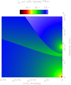
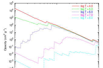
Figure 2: The main ingredients involved in the construction of models of the X-ray emission from colliding wind systems which are largely adiabatic. Top left: a density plot from a hydrodynamical model of the wind-wind collision. Top right: cooling curves for hot, thermal plasma. Bottom left: emissivity data (for solar abundances). Bottom right: opacity data (for solar abundances).

Early numerical models were presented by (amongst others) Lebedev & Myasnikov (1988), Luo, McCray & Mac Low (1990), and Stevens, Blondin & Pollock (1992). The main ingredients involved in these models are summarized in Fig. 2. A hydrodynamical code is used to model the dynamics of the WCR. In this example the deflection of the WCR by the orbital motion of the stars is assumed to be negligible, the WCR remains axis-symmetric, and a 2D $(r,z)$ calculation is performed. A small amount of artificial viscosity is used in the calculations to prevent the development of the odd-even decoupling (i.e. carbuncle) instability at the apex of the collision zone. This numerical artifact develops when shocks are locally aligned with the hydrodynamic grid (Walder, 1994; Le Veque, 1998). In Fig. 2, $\eta=0.1$, and the stellar winds were assumed to have reached their terminal speeds. We also specified $v_{\rm WR}=v_{\rm O}$, so the velocity shear along the contact discontinuity is small and there is no noticeable development of the Kelvin-Helmholtz instability (instabilities are discussed in greater detail in Sec. 5.3). In systems where the WCR is largely adiabatic, it is not strictly necessary to compute the rate of energy loss of the shocked gas through radiative cooling (since by definition this is small). However, it is often included in order that models are self-consistent. The hot plasma is generally assumed to be optically thin and in collisional ionization equilibrium, in which case the cooling rate as a function of temperature may be calculated using, for example, the MEKAL plasma emission code (Mewe, Kaastra & Liedahl, 1995).

Cooling curves for solar abundances ($X$[H]$=0.705$, $Y$[He]$=0.205$, $Z$[everything else]$=0.020$) and the abundances found for the WC8 star in $\gamma^{2}$ Vel ($X=0.0$, $Y=0.628$, $Z=0.372$) are shown in the top right panel of Fig. 2. Line emission dominates the cooling at temperatures below $10^{7}{\rm\thinspace K}$. At higher temperatures cooling occurs primarily through thermal bremsstrahlung ($\Lambda(T)\propto T^{1/2}$). The enhanced metal abundance in the winds of WR stars leads to more efficient cooling than is obtained for material of solar abundance.

To obtain synthetic X-ray data the hydrodynamical model is processed through a ray-tracing code which solves the radiative transfer equation along lines of sight through the hydrodynamical grid. Emissivity and opacity data for solar abundance material are shown in the bottom left and right panels of Fig. 2, respectively. The emissivity data was again calculated using the MEKAL code, and consists of line emission plus thermal bremsstrahlung continuum. At $T=10^{8}{\rm\thinspace K}$ most elements are completely ionized and there is little line emission in comparison to lower temperatures, while the bremsstrahlung emission extends to higher energies. The opacity data in the bottom right panel of Fig. 2 was calculated using the Cloudy photoionization code(Ferland, 2001). Distinct absorption edges are clearly visible. As the temperature increases and elements become more and more ionized the absorption cross-section decreases.

Once synthetic spectra and images have been calculated they can be compared against actual X-ray data, and the properties of CWBs determined. The most rigorous method involves the calculation of a grid of synthetic X-ray data from a large number of hydrodynamical models in which the stellar wind parameters are systematically varied. An XSPEC table model of the synthetic X-ray data grid can then be generated, and fitted against actual observational data. Constraints on the stellar mass-loss rates and wind terminal speeds have been obtained by this method for $\gamma^{2}$ Vel (Stevens et al., 1996), WR 140 (Zhekov & Skinner, 2000), and $\eta$ Carinae (Pittard & Corcoran, 2002). In each of these works the X-ray derived mass-loss rate for the star with the stronger wind is substantially lower than the best estimate from radio observations at that time. This is largely due to the fact that the X-ray derivation appears to be insensitive to wind clumping (unlike radio-based derivations of ${\dot{M}}$). The X-ray based method also enjoys further advantages. For instance, in the case of $\eta$ Carinae the high energy X-ray’s are much less affected by the complex circumstellar environment than emission at longer wavelengths. An additional benefit over other techniques is the ability to place constraints on the properties of the star with the weaker wind.

To illustrate this method at work, Fig. 3 shows a fit to a Chandra grating spectrum of $\eta$ Carinae (reproduced from Pittard & Corcoran, 2002). $\eta$ Carinae is arguably the most infamous massive star in our Galaxy, being best known as the survivor of the greatest non-terminal stellar explosion ever recorded. The ejecta have since formed the beautiful bipolar nebula known as the Homunculus (see, e.g., Morse et al., 1998). Study of this nebula (see, e.g., Smith et al., 2003) plays a central role in the quest for a deeper understanding of this object. Unfortunately, it seems that astronomers cannot have their cake and eat it, since the nebula also acts as a screen which significantly obscures the central star. For a long time $\eta$ Carinae was thought to be a single massive star and was classified as an luminous blue variable (LBV), but there is now overwhelming evidence for binarity and a strong wind-wind collision in this system (Damineli et al., 2000; Corcoran et al., 2001). Tantalizing evidence also exists to relate the “Great Eruption” in 1843 with the close approach of the stars during their passage through periastron. Whether the tidal influence of the companion star was in part responsible for triggering the enormous outburst is one of the most important questions concerning $\eta$ Carinae today.

$\eta$ Carinae is in fact a highly unusual example of a CWB. It may be the only one known in which one of the components is an LBV star (although HD 5980 may be another - see, e.g. Nazé et al., 2002), and as such the low wind speed of the primary star ($v\sim 500\hbox{${\rm{\rm\thinspace km}{\rm\thinspace s}^{-1}\,}$}$) means that the hard X-ray emission (above $2{\rm\thinspace keV}$) is generated almost exclusively by shocked material from the secondary wind. At the time of the Chandra observation (shown in Fig. 3) the attenuation of this hard emission by the stellar winds is small and the line of sight into the system is through the less dense wind of the companion star. This gives rise to the unusual situation that the hard X-ray emission is not directly sensitive to the mass-loss rate of the primary, but only indirectly through the wind momentum ratio $\eta$. Fortunately, the duration of the lightcurve minimum can be used to estimate $\eta$. The best fit to the X-ray data then gives $\hbox{${\dot{M}}$}\approx 10^{-5}\hbox{${\rm\hbox{${\rm\thinspace M_{\odot}}$}{\rm\thinspace yr}^{-1}\,}$}$ for the secondary star and $v\approx 3000\hbox{${\rm{\rm\thinspace km}{\rm\thinspace s}^{-1}\,}$}$ for its wind. With $\eta=0.2$ and assuming $v\sim 600\hbox{${\rm{\rm\thinspace km}{\rm\thinspace s}^{-1}\,}$}$ for the wind of the primary star, the fit in Fig. 3 implies $\hbox{${\dot{M}}$}\approx 2.5\times 10^{-4}\hbox{${\rm\hbox{${\rm\thinspace M_{\odot}}$}{\rm\thinspace yr}^{-1}\,}$}$ for the primary star. As noted earlier, this value is substantially smaller than commonly inferred (in the literature there is a large scatter in the derived values, though the general view is that $\hbox{${\dot{M}}$}\sim 10^{-3}\hbox{${\rm\hbox{${\rm\thinspace M_{\odot}}$}{\rm\thinspace yr}^{-1}\,}$}$). However, some problems with a mass-loss rate as high as $10^{-3}\hbox{${\rm\hbox{${\rm\thinspace M_{\odot}}$}{\rm\thinspace yr}^{-1}\,}$}$ have been identified: fits to HST data show absorption components which are too strong and electron-scattering wings which were overestimated (Hillier et al., 2001). Likewise, the X-ray derived results face their own set of problems. For instance, the derived wind parameters of the secondary star suggest that it is either a very massive O-star or perhaps a WR star, but no evidence for a companion has been found to date in optical spectra. It will be interesting, therefore, to see if the results in Pittard & Corcoran (2002) are consistent with those from further X-ray observations. Analysis of additional Chandra spectra taken through periastron passage is ongoing, and we hope to report results soon.

Figure 3: The best fit to a Chandra grating spectrum of $\eta$ Carinae (from Pittard & Corcoran, 2002). If we take the terminal speed of the primary wind as $v_{1}=600\;\hbox{${\rm{\rm\thinspace km}{\rm\thinspace s}^{-1}\,}$}$, then the fit implies that $\hbox{${\dot{M}}$}_{1}=2.5\times 10^{-4}\;\hbox{${\rm\hbox{${\rm\thinspace M_{\odot}}$}{\rm\thinspace yr}^{-1}\,}$}$.

Since the launch of Chandra and XMM-Newton, it has also become possible to measure the shift and width of individual X-ray lines from CWBs. The high spectral resolution offered by the gratings on these telescopes allows access to a wide range of important diagnostic data which can be used to place additional constraints on the wind-wind collision. The theoretical study of line profiles in CWBs is in its infancy, although some unexpected results have already been obtained. We refer the interested reader to Henley et al. (these proceedings).

3.2 Modeling X-ray emission from highly radiative systems

It is impossible to use the techniques described in the previous section when the shocked gas is highly radiative because in order to calculate the emission the cooling length must be spatially resolved. Hydrodynamical models (including those with adaptive-mesh-refinement) impose a limit to the spatial resolution which can be much larger than the cooling length of the gas in such systems. Another problem is that the rapid cooling of hot gas creates cold dense sheets which are unstable to a variety of instabilities (see, e.g., Stevens, Blondin & Pollock, 1992), and which introduce a large time dependence into the computed emission.

These short-comings have been recently addressed by Antokhin, Owocki & Brown (2004). Their solution is to separate the calculation of the small-scale (local) cooling structure of the post-shock gas from the global structure of the wind ram-pressure balance surface, and to assume that these structures are time-independent. The steady-state shape of the contact discontinuity in a CWB has been comprehensively discussed in the literature (see references in Antokhin, Owocki & Brown, 2004), though in these works the winds were assumed to have reached their terminal speeds before colliding. However, as the post-shock gas becomes increasingly radiative with decreasing stellar separation, such models are most applicable to short-period systems where the wind speeds will often have not reached their terminal values at the interaction front. To account for this, Antokhin, Owocki & Brown (2004) assumed “beta” velocity laws in their model.

In the highly radiative limit, the timescale for shock heated material to cool is small compared to the flow time for material to advect along a substantial arc of the contact discontinuity, and the post-shock gas can be assumed to occupy a layer which is geometrically thin with respect to other scales in the system (e.g., the binary separation, and the radius of curvature of the contact discontinuity). The expansion of the shocked gas as it flows out of the system normally couples the internal evolution of the post-shock gas to the global wind-wind structure, since adiabatic cooling can then take place. However, with the above assumptions one can adopt an “on-the-spot” treatment of the radiative emission at each point along the interaction front, and the post-shock structure can be simplified to planar geometry.

To obtain the structure of the cooling layer, Antokhin, Owocki & Brown (2004) adopted an isobaric approximation. Assuming that the energy loss in the shocked gas is solely from radiative cooling, the rate of temperature decrease in the post-shock gas is given by,

$$\frac{5k}{2\mu m_{\rm p}}\rho v\frac{dT}{dl}=-n_{\rm e}n_{\rm H}\Lambda(T),$$ (5)

where $l$ is a distance from the shock front, and $\Lambda(T)$ is the cooling function. Equation 5 also gives the width of the cooling layer, and a schematic of the post-shock structure is shown in Fig. 4.

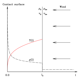
Figure 4: A schematic of the post-shock density and temperature structure in a steady, planar cooling layer (reproduced from Antokhin, Owocki & Brown (2004), with permission). The shock front occurs at $l_{0}$.

An example of the global structure of the WCR, together with the width of the post-shock cooling layer either side of the contact discontinuity, is shown in Fig. 5. An initial application of this method has been made to an XMM-Newton observation of the short-period binary HD 159176 (De Becker et al., 2004), with good success achieved in fitting the spectral shape. However, in this work it was not possible to obtain a good fit which was simultaneously in agreement with the predicted luminosity from the model.

This method shows great promise and it will clearly be useful to develop it further. Future work on this model could include extension to three dimentions (which would allow deflection of the interaction region into a spiral form as a result of orbital motion of the stars), and the dynamical role of the stellar radiation fields (see, e.g., Stevens & Pollock, 1994; Gayley, Owocki & Cranmer, 1997, and further discussion in Sec. 5). Further tests against a variety of short-period CWBs also need to be made, and in this respect XMM-Newton data from the archetype system V444 Cygni scheduled for May-June 2004 are ideally suited. It should also prove illuminating to compare the results from this method and those from hydrodynamical models in the transition region where $\chi\sim 1$.

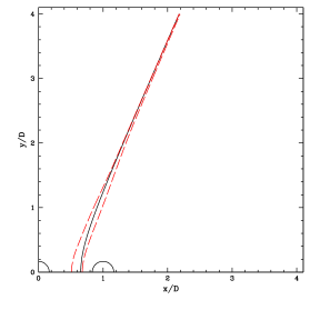
Figure 5: The structure of the wind-wind interaction from the model of Antokhin, Owocki & Brown (2004) (reproduced with permission). The solid line marks the contact discontinuity, while the dashed lines indicate the shock fronts.

4 Radio emission from early-type stars

Radio observations of early-type stars reveal that they can emit both thermal and nonthermal radiation. The former is readily explained as arising from free-free emission within the strong stellar wind (Wright & Barlow, 1975). The winds of early-type stars are partially optically thick at radio wavelengths, and the optical depth at radius $r$ is given by

$$\tau_{\nu}(r)\approx\int^{\infty}_{r}10^{-4}\left(\frac{Z^{2}\gamma_{e}}{\mu_{i}^{2}}\right)\left(\frac{\hbox{${\dot{M}}$}}{v_{\infty}}\right)^{2}\frac{g_{\nu}}{m_{\rm H}^{2}T^{3/2}\nu^{2}}\frac{1}{r^{4}}dr,$$ (6)

where $Z$ is the rms charge of the atoms ($Z=1$ for singly ionized gas), $\gamma_{e}$ is the number of free electrons per ion, $\mu_{i}$ is the mean atomic mass of the ions in units of $m_{\rm H}$, $g_{\nu}$ is the gaunt factor and $T$ is the temperature of the wind (see, e.g., Lamers & Cassinelli, 1999). The high mass-loss rate of massive stars means that the photospheric radius at radio wavelengths is always much larger than the radius of the underlying star. For an isothermal O-star wind with $T=10,000{\rm\thinspace K}$, $\hbox{${\dot{M}}$}=10^{-6}\hbox{${\rm\hbox{${\rm\thinspace M_{\odot}}$}{\rm\thinspace yr}^{-1}\,}$}$, $v_{\infty}=2000\hbox{${\rm{\rm\thinspace km}{\rm\thinspace s}^{-1}\,}$}$, and consisting mainly of ionized hydrogen, the $\tau_{\nu}=1$ surface occurs at radii of 1350, 1900 and $4200\hbox{${\rm\thinspace R_{\odot}}$}$ at radio wavelengths of 3.6, 6 and $20{\rm\thinspace cm}$ respectively. For WR stars, these radii are even larger. Since the wind speed is assumed to have reached its terminal value at these distances, radio observations have proved to be a useful tool for measurements of mass-loss rates (although as discussed in Sec. 3.1 these suffer from uncertainties due to the clumpy nature of such winds).

The nonthermal emission, on the other hand, is attributed to synchrotron radiation from relativistic electrons moving in a magnetic field. The consensus is that the relativistic electrons in the winds of massive stars are created through diffusive shock acceleration. In this process the electrons gain energy through the first-order Fermi mechanism as they cross and re-cross the shock until they are eventually scattered downstream (see, e.g., Bell, 1978). Electrons with Lorentz factor $\gamma\mathrel{\hbox to0.0pt{\lower 3.0pt\hbox{$\sim$}\hss}\raise 2.0pt\hbox{$<$}}10^{5}$ are frozen into the post-shock flow (White, 1985). The resulting energy distribution of the relativistic electrons has a power law form, i.e. the number of relativistic electrons per unit volume with energy between $\gamma$ and $\gamma+d\gamma$, $N(\gamma)\propto\gamma^{-n}$. The energy index, $n$, depends on the shock compression ratio, $\chi_{c}$, through (Bell, 1978)

$$n=\frac{\chi_{c}+2}{\chi_{c}-1}.$$ (7)

In the case where the shocked plasma radiates efficiently, the shock is quasi-isothermal, and the compression ratio can become very large, leading to $n\sim 1$. If instead the shock is adiabatic, then $\chi_{c}=4$ (for a strong shock), and $n=2$.

As already noted, hydrodynamical shocks are a feature of the winds of both single massive stars and their binary counterparts. In the case of single stars, the intrinsic instability of the radiatively driven wind leads to the formation of shocks which are distributed throughout the wind (see Runacres & Owocki, 2002, and references therein). While in principle these can accelerate electrons to high energies, the intense stellar radiation field causes significant energy losses through inverse Compton (IC) scattering and electrons accelerated in the inner regions of the stellar wind cannot survive out to large radii. Those electrons which are responsible for the nonthermal radio emission must therefore be accelerated at large distances from the star (Chen & White, 1994). The large photospheric radii of massive stars at radio wavelengths imposes a similar constraint, since for nonthermal emission to be observed at radio wavelengths, the relativistic electrons must exist outside the radio photospheric radius of the stellar wind.

In binary systems the strong shocks formed by the collision of the two winds is a natural place for diffusive shock acceleration of nonthermal electrons. Another possibility concerns the current sheets which result from the collision of magnetized stellar winds (Jardine, Allen & Pollock, 1996). The compression of magnetic field lines in the current sheets create enhanced local field strengths, and the resulting electric fields may accelerate particles to high energies. Irrespective of which is the dominant acceleration mechanism, wide binary systems have the significant advantages that the wind collision may exist well outside the radio photosphere of the stars, and that the stellar radiation energy density is substantially diluted in the vicinity of the WCR. This is reflected in strong observational support for a CWB interpretation for all synchrotron emission from WR stars (Dougherty & Williams, 2000), though the case is not so clear for O-stars (see, e.g., Rauw et al., 2002).

However, when synchrotron emission is not detected, that does not mean it is not being emitted. Nonthermal radio emission generated in the WCR of a short period binary may be buried so deep under the radio photosphere that the heavy opacity prevents its observation. For the nonthermal emission to be highly visible we require that the binary is wide enough that the apex of the WCR is far enough away from the stars that it exists outside of their radio photospheres. This separation implies a value of the orbital period of order of a month. Therefore, there is a selection effect that all the CWBs with observed synchrotron are wide binaries.

4.1 Modeling the radio emission from CWBs

Most analysis of the radio spectra from colliding wind binaries has hitherto been based on a highly simplified model consisting of a thermal source plus a point-like source of nonthermal emission attenuated by free-free absorption (e.g., Chapman et al., 1999; Monnier et al., 2002). In this model, at frequency $\nu$, the observed flux ($S_{\nu}^{\rm obs}$) is related to the thermal flux ($S_{\nu}^{\rm th}$), the synchrotron emission arising from the WCR ($S_{\nu}^{\rm syn}$), and the free-free opacity ( $\tau_{\nu}^{\rm ff}$) of the circum-system stellar wind envelope by

$$S_{\nu}^{\rm obs}=S_{\nu}^{\rm th}+S_{\nu}^{\rm syn}{\rm e}^{-\tau_{\nu}^{\rm ff}}.$$ (8)

From simultaneous measurements in a number of frequency bands it is possible to solve Eq. 8 to determine the relative contribution of thermal and nonthermal emission to the total flux. On the other hand, both $S_{\nu}^{\rm syn}$ and $\tau_{\nu}^{\rm ff}$ may display significant time variability. The former is expected if the stellar separation varied as in an eccentric binary, while the latter is in general anticipated since the optical depth to the synchrotron emitting region will change as the line of sight sweeps around the system.

While Eq. 8 may at times be adequate, a single-valued free-free opacity determined along the line-of-sight to a point-like synchrotron emission region is a clear over-simplification: observations reveal an extended region of synchrotron emission from both WR 146 (Dougherty et al., 1996; Dougherty, Williams & Pollacco, 2000) and WR 147 (Moran et al., 1989; Churchwell et al., 1992; Williams et al., 1997) - see also Sec. 4.1.1. Furthermore, use of such over-simplified models has often resulted in difficulties in fitting observational data. Nowhere are these problems better illustrated than for the wonderful dataset which exists for WR 140, the archetype wide CWB (see, e.g., Williams et al., 1990; White & Becker, 1995). We note that the effect of binarity on the thermal radio emission from massive stars has also been investigated (Stevens, 1995), though this work did not examine nonthermal emission.

Complex magnetohydrodynamic models which include the transport of nonthermal electrons have been computed to predict the synchrotron emission from other astrophysical objects, such as radio jets (Tregillis, Jones & Ryu, 2004). However, less attention has been focused on models for CWBs, and the resulting models are less well developed. In fact, CWBs are nice laboratories for particle acceleration because the fundamental flow parameters of the winds are well known.

As a first step towards the construction of more realistic models, Dougherty et al. (2003) obtained a simple representation of the spatial distribution of the free-free and nonthermal emission from CWB systems through the use of a hydrodynamical model of the WCR. In this section we note the main results of this work.

Figure 6: Spectra from the standard model with $0^{\circ}$ inclination - free-free flux (dashed), magneto-bremsstrahlung flux (dotted), and total flux (solid). IC cooling, coulombic cooling, the Razin effect and synchrotron self absorbtion (SSA) are not included in this calculation.

The process of calculating the theoretical radio emission from a hydrodynamical model of a CWB is as follows. First, the temperature and density values on the hydrodynamic grid are used to calculate the free-free emission and absorption coefficients from each grid cell. The synchrotron emission and synchrotron self-absorption from each cell within the WCR is calculated assuming that the distribution of relativistic electrons in each cell can be specified by $N(\gamma)d\gamma=C\gamma^{-p}d\gamma$, where $p=2$. The standard assumption that $C$ is proportional to the thermal energy density is made (c.f. Chevalier, 1982; Mioduszewski, Dwarkadas & Ball, 2001), and it is assumed that $p$ is spatially invariant over the volume of the WCR. The magnetic field in the WCR is assumed to be highly tangled, and the synchrotron emissivity ($P_{\nu}\propto\nu^{-(p-1)/2}$) is assumed to be valid over all frequencies, $\nu$. A radiative transfer calculation is then computed to obtain the flux and intensity distribution at a specified frequency. The interested reader is referred to Dougherty et al. (2003) for further details.

Table 3: Parameters for the “standard” CWB model in Dougherty et al. (2003).

Parameter	Value
$\hbox{${\dot{M}}$}_{\rm WR}\;(\hbox{${\rm\hbox{${\rm\thinspace M_{\odot}}$}{\rm\thinspace yr}^{-1}\,}$})$	$2\times 10^{-5}$
$\hbox{${\dot{M}}$}_{\rm O}\;(\hbox{${\rm\hbox{${\rm\thinspace M_{\odot}}$}{\rm\thinspace yr}^{-1}\,}$})$	$2\times 10^{-6}$
$v_{\infty,{\rm WR}}\;(\hbox{${\rm{\rm\thinspace km}{\rm\thinspace s}^{-1}\,}$})$	$2000$
$v_{\infty,{\rm O}}\;(\hbox{${\rm{\rm\thinspace km}{\rm\thinspace s}^{-1}\,}$})$	$2000$
$D\;({\rm\thinspace cm})$	$2\times 10^{15}$

We shall first discuss the results obtained from a “standard” CWB model with the parameters noted in Table 3. These wind values are typical of WR and OB stars, and with the adopted binary separation, $D$, the WCR is largely adiabatic. At a frequency $\nu=5\;{\rm GHz}$, $D$ is approximately $10\times$ the radius of the $\tau_{\rm ff}=1$ surface of the WR wind. For inclination angles $\sim$$0^{\circ}$, the lines of sight to the WCR are then optically thin, permitting investigation of the emission from the wind-collision region in the absence of strong free-free absorption from the circum-binary stellar wind envelope. Solar abundances for the O-star and WC-type abundances for the WR-star (mass fractions $X=0,Y=0.75,Z=0.25$) are adopted in the model. Temperatures of $10,000$ K and an ionization structure of ${\rm H^{+}}$, ${\rm He^{+}}$ and ${\rm CNO^{2+}}$ are assumed for the unshocked stellar winds, and the system is assumed to be positioned at a distance of 1.0 kpc. Finally, it is assumed that the magnetic energy density, $U_{B}$, the relativistic electron energy density, $U_{\rm rel}$, and the thermal energy density, $U_{\rm th}$, are related by

$$U_{\rm B}=\frac{B^{2}}{8\pi}=\zeta_{\rm B}U_{\rm th},$$ (9)

and

$$U_{\rm rel}=\int n(\gamma)\gamma mc^{2}d\gamma=\zeta_{\rm rel}U_{\rm th},$$ (10)

where $\zeta_{\rm B}$ and $\zeta_{\rm rel}$ are constants, and $U_{\rm th}={P\over{\Gamma-1}}$ where $P$ is the gas pressure and $\Gamma$ is the adiabatic index (assumed to be $5/3$, as for an ideal gas). The common assumption of equipartition corresponds to $\zeta_{\rm B}=\zeta_{\rm rel}=\zeta$. The nonthermal electrons lose energy due to synchrotron emission and IC scattering in the same ratio as the magnetic field energy density to the photon energy density,

$$\frac{P_{\rm sync}}{P_{\rm compt}}=\frac{U_{\rm B}}{U_{\rm ph}}.$$ (11)

For all reasonable values of $\zeta_{\rm B}$, $P_{\rm sync}<P_{\rm compt}$, and IC cooling is the dominant energy loss mechanism. Synchrotron cooling is therefore ignored.

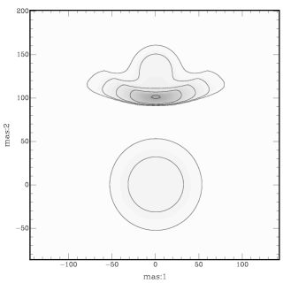
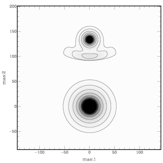
Figure 7: Intensity distributions from the standard model at $0^{\circ}$ inclination at 1.6 GHz (top) and 22 GHz (bottom). Neither IC cooling, coulombic cooling, the Razin effect or SSA, are included in this calculation. The stellar winds and the WCR are clearly visible.

Table 4: Values from the “standard” CWB model in Dougherty et al. (2003).

Parameter	Value
$n_{\rm max}\;(\hbox{${\rm{\rm\thinspace cm}^{-3}\,}$})$	$4\times 10^{5}$
$T_{\rm max}\;({\rm\thinspace K})$	$2\times 10^{8}$
$B_{\rm max}\;({\rm\thinspace mG})$	6

The maximum post-shock density, temperature, and B-field occur at the stagnation point between the stars and are listed in Table 4. The synchrotron emission arising from a single relativistic electron with Lorentz factor $\gamma$ is (c.f. Rybicki & Lightman, 1979)

$$P(\nu)=\frac{\sqrt{3}q^{3}B{\rm sin}\alpha}{\rm m_{e}c^{2}}F(\nu/\nu_{c}),$$ (12)

where $q$ is the electron charge, $B$ is the magnetic field strength, $\alpha$ is the pitch angle of the particle relative to the direction of the B-field, ${\rm m_{e}}$ is the mass of the electron, $c$ is the speed of light, and $F(\nu/\nu_{c})$ is a dimensionless function describing the total power spectrum of the synchrotron emission, with $\nu_{c}$ the frequency where the spectrum cuts off, given by

$$\nu_{\rm c}=\frac{3\gamma^{2}qB{\rm sin}\alpha}{\rm 4\pi m_{e}c}.$$ (13)

Values for $F(\nu/\nu_{c})$ are tabulated in Ginzburg & Syrovatskii (1965) and we assume that ${\rm sin}~{}\alpha=1$. At the stagnation point $\nu_{\rm c}=0.25$ GHz (for $\gamma=10^{2}$) and 25 GHz (for $\gamma=10^{3}$).

The spectra and intensity distributions obtained from the standard model with $\zeta=10^{-4}$ are shown in Fig. 6 and Fig. 7 respectively where, for simplicity, only free-free absorption is included. Magneto-bremsstrahlung emission dominates the total flux below 1 GHz. The turnover seen near 400 MHz is due to free-free absorption from the unshocked stellar winds. Above 400 MHz, the magneto-bremsstrahlung spectrum is a power-law with a spectral index ($S_{\nu}\propto\nu^{\alpha}$) $\alpha=-0.5$, as expected for a $p=2$ energy distribution. The thermal spectrum spectral index of $+0.6$ is also as expected, though a slight departure from a power-law exists at low frequencies due to the finite size of the hydrodynamical grid. The intensity distributions shown in Fig. 7 reveal that at 1.6 GHz the WCR is brighter than the stellar winds, while the opposite is true at 22 GHz.

Dougherty et al. (2003) also explored how the radio flux varied with stellar separation, and we repeat the main conclusions here. We shall first consider how varying the stellar separation affects the free-free opacity to a specific point in the WCR. For a stellar wind with an $r^{-2}$ radial density distribution the line-of-sight opacity $\tau$, at frequency $\nu$ through the wind is $\tau\propto\xi^{-3}\nu^{-2.1}$, where $\xi$ is the impact parameter. Since $\xi\propto D$ for a given inclination, the turnover frequency for a constant opacity value is $\nu\propto D^{-10/7}$. Dougherty et al. (2003) showed that this relationship is in excellent agreement with the data shown in their Fig. 5.

Now let us consider how the intrinsic synchrotron emission depends on the stellar separation. In the absence of synchrotron self absorbtion (SSA) or the Razin effect, the synchrotron luminosity increases as the separation decreases, due to the increased thermal energy density in the collision region. In this scenario, the intrinsic synchrotron emission per unit volume $P(\nu)\propto\zeta^{3/4}n^{3/4}\nu^{-1/2}$ for an electron power-law index $p=2$. Since the post-shock density $\propto D^{-2}$ and the volume of the emitting region scales as $D^{3}$, the total synchrotron emission from the entire wind collision volume scales as $D^{-1/2}\nu^{-1/2}$, as noted by Dougherty et al. (2003) and displayed in their Fig. 6.

Figure 8: The radio spectrum of WR 147. The deduced synchrotron emission is represented by solid data points, while the total flux is represented by the hollow data points. Estimates from different authors are as follows: solid squares (two separate estimates from the same observational data, Skinner et al., 1999), solid pentagons (Setia Gunawan et al., 2001), open circles (Churchwell et al., 1992; Contreras & Rodríguez, 1999). The lines are the total (solid), thermal (dotted) and synchrotron (dot-dashed) spectra of the $i=0^{\circ}$ model with $\zeta=7.03\times 10^{-3}$, where SSA, Razin and free-free absorption are included in the radiative transfer calculations. The model winds were assumed to be clumpy with a volume-filling factor $f=0.134$. Models at $+30^{\circ}$ and $-30^{\circ}$ are also consistent with the data.

4.1.1 Modeling the radio emission from WR 147

WR 147 is notable for being among the brightest WR stars at radio frequencies, and for being one of two systems in which the thermal and synchrotron emission are observed to arise from two spatially resolved regions (see, e.g., Williams et al., 1997, and references therein). Furthermore, it is one of a handful of WR+OB binary systems where the two stars are resolved into a visual pair (Niemela et al., 1998; Williams et al., 1997) with a projected stellar separation given by $D\cos~{}i=0.635\pm 0.020$$.\!\!^{\prime\prime}$. At the estimated distance of $\sim$0.65 kpc (Churchwell et al., 1992; Morris et al., 2000) this corresponds to a separation $D\sim 415/\cos~{}i$ AU, and the relationship between $D$ and $i$ represents an important constraint for any models of the system. As the inclination angle is unknown, Dougherty et al. (2003) investigated models for several different values of $i$, which in turn requires different values of the physical separation, $D$, to maintain the observed angular separation.

The radio spectrum of WR 147 is perhaps the best observed of all massive binary systems, with radiometry extending from 353 MHz to 42.9 GHz. However, differences in excess of 50% exist in the derived synchrotron flux at some frequencies (cf. Fig. 8), giving rise to uncertainty in the position of the low frequency turnover (see Dougherty et al., 2003, for further details). These differences form the fundamental reason for conflicting conclusions about the nature of the underlying electron energy spectrum in the current literature (Skinner et al., 1999; Setia Gunawan et al., 2001).

Full details of the modeling of the radio spectrum of WR 147 can be found in Dougherty et al. (2003). Values for the mass-loss rates of the stars, and the terminal velocities of the winds are noted in Table 5. These were taken from the literature, as were details of the wind compositions. The temperature for both stellar winds was assumed to be 10 kK, and the dominant ionization states were taken to be H⁺, He⁺ and CNO²⁺. The thermal flux is only weakly dependent on the assumed wind temperature (through the Gaunt factor), if the ionization state is fixed.

Table 5: Parameters for the WR 147 model in Dougherty et al. (2003).

Parameter	Value
$\hbox{${\dot{M}}$}_{\rm WN8}\;(\hbox{${\rm\hbox{${\rm\thinspace M_{\odot}}$}{\rm\thinspace yr}^{-1}\,}$})$	$2\times 10^{-5}$
$\hbox{${\dot{M}}$}_{\rm OB}\;(\hbox{${\rm\hbox{${\rm\thinspace M_{\odot}}$}{\rm\thinspace yr}^{-1}\,}$})$	$3.8\times 10^{-7}$
$v_{\infty,{\rm WN8}}\;(\hbox{${\rm{\rm\thinspace km}{\rm\thinspace s}^{-1}\,}$})$	$950$
$v_{\infty,{\rm OB}}\;(\hbox{${\rm{\rm\thinspace km}{\rm\thinspace s}^{-1}\,}$})$	$1000$

Models with $i=0$, 30 and $60^{\circ}$ were computed, and values of $\zeta$ were estimated for each model by matching the mean of the “observed” synchrotron 4.86 GHz fluxes, which was taken to be $14.1\pm 0.3$ mJy. The spectrum between 0.2 and 80 GHz was then calculated assuming this constant value of $\zeta$. To fit the thermal flux with the chosen value of ${\dot{M}}_{\rm WN8}$ the winds were required to be clumped.

In Fig. 8 the resulting total, synchrotron and thermal spectra from one of the models ($i=0$, and including SSA, the Razin effect and free-free absorption) is shown against the observed spectra. Though this is not the best fit to the data in a formal sense, the model fits the data reasonably well given the approximations and assumptions which it contains. The shortcomings are that the total flux in the 5 to 8 GHz range is underestimated, and the synchrotron emission does not turn down somewhere around 10 to 20 GHz as suggested by the observed data. The shortfall in the 5-8 GHz total flux could be eliminated by increasing the thermal emission by a few mJy. This could be achieved by simply increasing $\hbox{${\dot{M}}$ }/v_{\infty}$ in the stellar winds. While this would require that the synchrotron emission at frequencies higher than $\sim$ 10 GHz be lower than in the current models, this may well be the case if IC cooling is taken into account, as explained below.

The fit shown in Fig. 8 has $\zeta\approx 7\times 10^{-3}$, which implies that $B_{\rm max}=4{\rm\thinspace mG}$. If the tangled field in the WCR has its origin in the O-star photosphere we deduce that the B-field at the surface of the O-star is $B_{*}\sim 100$ G. This is comparable with the non-detection of the Zeeman effect for the majority of OB stars which puts an upper limit $\sim 100$ G on $B_{*}$ (Mathys, 1999). It is also worth noting that it is assumed that the nonthermal electron energy density is in equipartition with the magnetic and thermal energy densities. Since the energy density of nonthermal protons, $U_{\rm p}$, is likely to be $50\times$ higher than that of the electrons, the deduced value of $\zeta\approx 7\times 10^{-3}$ means that $U_{\rm p}$ is uncomfortably close to unity. If the shocks in CWBs really are this efficient at accelerating particles, the thermal properties of the shock-heated, X-ray emitting gas will be affected. It is interesting to note that X-ray spectra from CWBs has to date always been modeled and interpreted assuming that the shocks place an insignificant fraction of their energy in relativistic particles, so this finding has implications for the analysis of X-ray data.

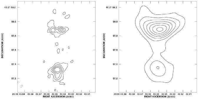
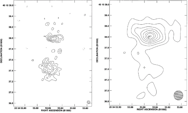
Figure 9: Intensity distributions at 4.8 (left) and 1.6 GHz (right) of our WR 147 model at $0^{\circ}$ inclination (top panels) and the actual observations reproduced from Williams et al. (1997) (bottom panels). The simulated MERLIN observations use the same u-v distribution and beam sizes as the actual observations in the bottom panels. The beams are circular, of diameter 57 and 175 mas at 4.8 and 1.6 GHz respectively. The contour levels in the simulated and actual images are also the same. The similarity of the simulated and actual observations is striking.

To appreciate how the intensity distributions from the models compare with the MERLIN observations shown in Williams et al. (1997), visibilities were generated from the model intensity distributions. The resulting visibilities were then imaged and deconvolved using the same procedure as in Williams et al. (1997), giving the “simulated” observations shown in the upper panels of Fig. 9. The remarkable similarity between these images and the actual observations shown in the lower panels of Fig. 9 is striking. However, a critical eye reveals that the 5 GHz peak intensity of the collision region is a little lower than that of the WR stellar wind in the model, and the WR star is a little too bright at 1.6 GHz. The WR star also appears to be a little more compact than the observations show, and we attribute these minor differences to our simple spherical, isothermal model of the stellar winds. Note that the OB star is not visible in the simulated observations. This is because the observations are essentially the intensity distribution convolved with the interferometer beam and the emission from the OB star is then sufficiently dispersed that it is no longer visible.

Examination of the simulated images can help to constrain the inclination angle. The synthetic observations shown in Fig. 9 are for an inclination of $0$$.\!\!^{\circ}$ At an inclination angle of $30^{\circ}$, the synchrotron emission is spread out over a much larger area and has a much lower surface brightness than in the simulation for $i=0^{\circ}$, and in the actual observations. This fact, and the spectral modeling, points to a fairly low value for the system inclination, between $0^{\circ}$ and $30^{\circ}$, though this is contrary to the conclusions of Pittard et al. (2002) where larger inclination angles were required to recover the extended X-ray emission. This apparent contradiction may be resolved if the stellar X-ray emission is extended on larger scales than previously thought (see Skinner et al., 2002).

5 Additional considerations and future perspectives

In this section we briefly review processes which, though important, have not been discussed elsewhere in this paper. We refer the interested reader to Folini & Walder (2000) where some of these effects are discussed in greater detail, including speculations on their mutual interaction. Theoretical considerations for clumped winds and the intriguing problem of dust formation are discussed in Folini & Walder (2000) and Walder & Folini (2002).

5.1 Radiation dynamics

The influence of one star’s radiation field on the dynamics of the other star’s wind has been quantified by Stevens & Pollock (1994) and Gayley, Owocki & Cranmer (1997, Pittard, 1998, see also). In close binaries the winds may be inhibited in their initial acceleration (since the net radiation flux is reduced between the stars). In WR+O binaries, where the WCR occurs closer to the O star than the WR star, the WR wind may be rapidly braked if there is strong coupling with the O-star radiation field. The opening angle of the WCR is a sensitive diagnostic of the braking effect, although the geometry of the WCR is an ambiguous constraint when the momentum ratio, $\eta$, of the winds is not known. The reduction in pre-shock velocity and the change to the morphology of the WCR have obvious consequences for the X-ray emission, but should also impact the radio emission.

5.2 Orbit-induced curvature of the WCR

Orbital motion will distort the structure of the WCR into a large-scale spiral form, and is strikingly displayed in infrared observations of WR 104 (Tuthill, Monnier & Danchi, 1999). Theoretical models of the curvature range from the analytical (Cantó et al., 1999; Tuthill et al., 2003), to the numerical (Williams, van der Hucht & Spoelstra, 1994), to the hydrodynamical (Pittard & Stevens, 1999; Walder & Folini, 2003). The orbit-induced curvature of the WCR will affect the observed X-ray emission in close binaries (Pittard, 2002) and the radio emission seen from wider (especially eccentric) binaries. Theoretical simulations are currently thin on the ground.

5.3 Instabilities

The WCR is subject to many different types of instability. These include the classical Rayleigh-Taylor, Kelvin-Helmholtz and Richtmyer-Meshkov instabilities which act on the surface between the two winds, thin-shell instabilities which act on isothermal shock-bounded slabs (Vishniac, 1994; Blondin & Marks, 1996), and the thermal instability from radiative cooling (e.g., Strickland & Blondin, 1995). Since these instabilities are not isolated from one another, the resulting flow may be very complex (see, e.g., Stevens, Blondin & Pollock, 1992). While the degree of instability in theoretical models may depend on assumptions made in the hydrodynamical code (see Myasnikov, Zhekov & Belov, 1998), it seems certain that the WCR will often be dynamically unstable. This may lead to some X-ray (Pittard & Stevens, 1997) and radio variability.

5.4 Ionization equilibrium

It is generally assumed that the shocked gas is in ionization equilibrium, though in wide binaries there could be some departure from this (see discussion in Henley et al. in these proceedings). The self-consistent inclusion of non-equilibrium ionization has yet to be incorporated into hydrodynamical models of CWBs. It will be interesting to discover if future work in this direction is able to better reproduce the X-ray line shifts seen in WR 140 where inconsistencies with current models exist.

5.5 Ion-electron temperature

In wide binaries the shocks will be collisionless, and the immediate post-shock electron and ion temperatures may differ. This possibility has been investigated in a preliminary fashion by Zhekov & Skinner (2000), where the effect on the X-ray emission from the WCR in WR 140 was examined. While the broad-band spectral fits to ASCA data indicated that a model with this effect was preferred, it is probably too soon to draw strong conclusions from this work and further study is needed.

5.6 Thermal conduction

There has been little work to date on thermal conduction in CWBs. However, the high temperatures and the steep temperature gradients in these systems indicate that thermal conduction may play an important role. Preliminary work has been carried out by Myasnikov & Zhekov (1998), Motamen, Walder & Folini (1999), and Zhekov & Myasnikov (2003), where it is shown that efficient thermal conduction increases the X-ray luminosity and softens its spectrum. However, the presence of magnetic fields greatly reduces the thermal conductivity in a direction perpendicular to the field lines, and this has not yet been considered. This should be addressed in future work since we know that magnetic fields are present in these systems due to the synchrotron emission which is observed.

5.7 IC cooling of nonthermal particles

While the simple models presented in Dougherty et al. (2003) are able to reproduce both the spectrum and the spatial distribution of radio emission remarkably well, the neglect of IC cooling is a major omission. To realistically model the observed radio emission from CWBs the downstream evolution of the nonthermal electron energy spectrum should be calculated. This is being addressed in a follow-up paper (Pittard et al., in preparation) where, in addition, the effect of Coulombic cooling on the lower energy relativistic particles is also considered.

5.8 IC cooling of thermal particles

IC losses may be important not only for the nonthermal shock-accelerated particles, but, at times, perhaps also for the hot post-shock thermal gas (see, e.g., White & Chen, 1995). More work is needed in this area to determine when this might lead to a significant change in the resulting thermal X-ray emission.

6 Summary

The wide range of parameter space covered by CWBs means that they are useful probes of a wide range of physical phenomena. X-ray observations in close binaries are a sensitive tool to study radiative braking, while in wide binaries X-ray emission is a useful diagnostic of the electron-ion temperature equilibration timescale. The input of theoretical X-ray spectra into XSPEC via user generated “table models” has proved to be extremely useful in obtaining direct constraints of the mass-loss rates of the binary components, and enjoys several advantages over more traditional techniques. Such work applied to $\eta$ Carinae may in future determine if there is enhanced stellar mass-loss associated with the periodic close approach of the stars.

On the other hand, radio observations can be used to explore the efficiency of diffuse shock acceleration at densities much higher than those in other astronomical objects with high Mach number shocks, e.g., supernovae. Preliminary work in this area indicates that it may be necessary to consider the effect of particle acceleration on the shock jump conditions. Another consequence of particle acceleration is that subsequent IC cooling of the relativistic particles leads to nonthermal emission at X-ray and $\gamma$-ray energies, e.g., Pollock (1987), Benaglia & Romero (2003). Such emission may already have been detected at X-ray energies (Rauw et al., 2002), and new and forthcoming missions like INTEGRAL and GLAST may observe this effect at $\gamma$-ray energies.

Future work should address these issues and those identified in Sec. 5, and where possible radio and X-ray data should be compared against theoretical predictions from a unified model. The review of (some) important processes and mechanisms in Section 5 demonstrates the richness of physical effects occurring in colliding wind binaries which we are striving to understand.

References

- Antokhin, Owocki & Brown (2004) Antokhin, I.I., Owocki, S.P., Brown, J.C. 2004, ApJ, submitted
- Bell (1978) Bell, A.R. 1978, MNRAS, 182, 147
- Benaglia & Romero (2003) Benaglia, P., Romero, G.E. 2003, A&A, 399, 1121
- Blondin & Marks (1996) Blondin, J.M., Marks, B.S. 1996, New Astr., 1, 235
- Cantó et al. (1999) Cantó, J., Raga, A., Keonigsberger, G., Moreno, E. 1999, in “Wolf-Rayet Phenomena in Massive Stars and Starburst Galaxies”, eds. K.A. van der Hucht, G. Koenigsberger & P.R.J. Eenens, IAU Symp. 193, 338
- Chapman et al. (1999) Chapman, J.M., Leitherer, C., Koribalski, B., Bouter, R., Storey, M. 1999, ApJ, 518, 890
- Chen & White (1994) Chen, W., White, R.L. 1994, Ap&SS, 221, 259
- Cherepashchuk (1976) Cherepashchuk, A.M. 1976, SvA Lett., 2, 138
- Chevalier (1982) Chevalier, R. A. 1982, ApJ, 259, 302
- Chlebowski & Garmany (1991) Chlebowski, T., Garmany, C.D. 1991, ApJ, 368, 241
- Churchwell et al. (1992) Churchwell, E., Bieging, J.H., van der Hucht, K.A., Williams, P.M., Spoelstra, T.A.T., Abbott, D.C. 1992, ApJ, 393, 329
- Contreras & Rodríguez (1999) Contreras, M.E., Rodríguez, L.F. 1999, ApJ, 515, 762
- Corcoran (1996) Corcoran, M.F. 1996, in Niemela V., Morrell N., eds, RMAA Conf. Ser. 5, Proceedings of the Workshop on Colliding Winds in Binary Stars. p. 54
- Corcoran et al. (2001) Corcoran, M.F., Ishibashi, K., Swank, J.H., Petre, R. 2001, ApJ, 547, 1034
- Corcoran et al. (2001) Corcoran, M.F. et al. 2001, ApJ, 562, 1031
- Damineli et al. (2000) Damineli, A., Kaufer, A., Wolf, B., Stahl, O., Lopes, D.F., de Araújo, F.X. 2000, ApJ, 528, L101
- De Becker et al. (2004) De Becker, M., et al. 2004, A&A, 416, 221
- Dougherty et al. (2003) Dougherty, S.M., Pittard, J.M., Kasian, L., Coker, R.F., Williams, P.M., Lloyd, H.M. 2003, A&A, 409, 217
- Dougherty & Williams (2000) Dougherty, S.M., Williams, P.M. 2000, MNRAS, 319, 1005
- Dougherty, Williams & Pollacco (2000) Dougherty, S.M., Williams, P.M., Pollacco, D.L. 2000, MNRAS, 316, 143
- Dougherty et al. (1996) Dougherty, S.M., Williams, P.M., van der Hucht, K.A., Bode, M.F., Davis, R.J. 1996, MNRAS, 280, 963
- Eichler & Usov (1993) Eichler, D., Usov, V. 1993, ApJ, 402, 271
- Ellison & Reynolds (1991) Ellison, D.C., Reynolds, S.P. 1991, ApJ, 382, 242
- Ferland (2001) Ferland, G.J. 2001, “Hazy, a brief introduction to Cloudy 96.00”
- Folini & Walder (2000) Folini, D., Walder, R. 2000, in “Thermal and Ionization Aspects of Flows from Hot Stars: Observations and Theory”, eds. H.J.G.L.M. Lamers and A. Sapar, ASP Conf. Ser. 204, 267
- Gayley, Owocki & Cranmer (1997) Gayley, K.G., Owocki, S.P., Cranmer, S.R. 1997, ApJ, 475, 786
- Ginzburg & Syrovatskii (1965) Ginzburg, V.L., Syrovatskii, S.I. 1965, ARA&A, 3, 297
- Hill et al. (2000) Hill, G.M., Moffat, A.F.J., St-Louis, N., Bartzakos, P. 2000, MNRAS, 318, 402
- Hillier et al. (2001) Hillier, D.J., Davidson, K., Ishibashi, K., Gull, T. 2001, ApJ, 553, 837
- Jardine, Allen & Pollock (1996) Jardine, M., Allen, H.R., Pollock, A.M.T. 1996, A&A, 314, 594
- Lamers & Cassinelli (1999) Lamers, H.J.G.L.M., Cassinelli, J.P. 1999, “Introduction to Stellar Winds” (Cambridge University Press)
- Le Veque (1998) Le Veque, R.J. 1998, “Nonlinear Conservation Laws and Finite Volume Methods”, in Saas-Fee Advanced Course 27: Computational Methods for Astrophysical Fluid Flow
- Lebedev & Myasnikov (1988) Lebedev, M.G., Myasnikov, A.V. 1988, in “Numerical Methods in Aerodynamics”, eds. V.M. Paskonov & G.S. Roslyakov, Moscow State University Press, Moscow, 3
- Luo, McCray & Mac Low (1990) Luo, D., McCray, R., Mac Low, M. 1990, ApJ, 362, 267
- Mathys (1999) Mathys, G. 1999, in “Variable and Non-spherical Stellar Winds in Luminous Hot Stars”, eds. B. Wolf, O. Stahl & A.W. Fullerton, Lecture Notes in Physics, 523, 95
- Mewe, Kaastra & Liedahl (1995) Mewe, R., Kaastra, J.S., Liedahl, D.A. 1995, Legacy, 6, 16
- Mioduszewski, Dwarkadas & Ball (2001) Mioduszewski, A.J., Dwarkadas, V.V., Ball, L. 2001, ApJ, 562, 869
- Moffat et al. (2002) Moffat, A.F.J., et al. 2002, ApJ, 573, 191
- Monnier et al. (2002) Monnier, J.D., Greenhill, L.J., Tuthill, P.G., Danchi, W.C. 2002, ApJ, 566, 399
- Moran et al. (1989) Moran, J.P., Davis, R.J., Spencer, R.E., Bode, M.F., Taylor, A.R. 1989, Nature, 340, 449
- Morris et al. (2000) Morris, P.W., van der Hucht, K.A., Crowther, P.A., et al. 2000, A&A, 353, 624
- Morse et al. (1998) Morse, J.A., Davidson, K., Bally, J., Ebbets, D., Balick, B., Frank, A. 1998, AJ, 116, 2443
- Motamen, Walder & Folini (1999) Motamen, S.M., Walder, R., Folini, D. 1999, in “Wolf-Rayet Phenomena in Massive Stars and Starburst Galaxies”, eds. K.A. van der Hucht, G. Koenigsberger & P.R.J. Eenens, IAU Symp. 193, 378
- Myasnikov & Zhekov (1998) Myasnikov, A.V., Zhekov, S.A. 1998, MNRAS, 300, 686
- Myasnikov, Zhekov & Belov (1998) Myasnikov, A.V., Zhekov, S.A., Belov, N.A. 1998, MNRAS, 298, 1021
- Nazé et al. (2002) Nazé, Y., et al. 2002, ApJ, 580, 225
- Niemela et al. (1998) Niemela, V.S., Shara, M.M., Wallace, D.J., Zurek, D.R., Moffat, A.F.J. 1998, AJ, 115, 2047
- Pittard (1998) Pittard, J.M. 1998, MNRAS, 300, 479
- Pittard (2002) Pittard, J.M. 2002, in “Interacting Winds from Massive Stars”, eds. A.F.J. Moffat and N. St-Louis, ASP Conf. Ser. 260, 627
- Pittard & Corcoran (2002) Pittard, J.M., Corcoran, M.F. 2002, A&A, 383, 636
- Pittard & Stevens (1997) Pittard, J.M., Stevens, I.R. 1997, MNRAS, 292, 298
- Pittard & Stevens (1999) Pittard, J.M., Stevens, I.R. 1999, in “Wolf-Rayet Phenomena in Massive Stars and Starburst Galaxies”, eds. K.A. van der Hucht, G. Koenigsberger & P.R.J. Eenens, IAU Symp. 193, 386
- Pittard & Stevens (2002) Pittard, J.M., Stevens, I.R. 2002, A&A, 388, L20
- Pittard et al. (2002) Pittard, J.M., et al. 2002, A&A, 388, 335
- Pollock (1987) Pollock, A.M.T. 1987, ApJ, 320, 283
- Pollock (1987) Pollock, A.M.T. 1987, A&A, 171, 135
- Pollock et al. (2004) Pollock, A.M.T., Corcoran, M.F., Stevens, I.R., Williams, P.M. 2004, ApJ, submitted
- Prilutskii & Usov (1976) Prilutskii, O.F., Usov, V.V. 1976, SvA, 20, 2
- Rauw, Vreux & Bohannan (1999) Rauw, G., Vreux, J.-M., Bohannan, B. 1999, ApJ, 517, 416
- Rauw et al. (2002) Rauw, G., et al. 2002, A&A, 394, 993
- Runacres & Owocki (2002) Runacres, M.C., Owocki, S.P. 2002, A&A, 381, 1015
- Rybicki & Lightman (1979) Rybicki, G.B., Lightman, A.P. 1979, “Radiative processes in astrophysics” (New York: Wiley-Interscience)
- Setia Gunawan et al. (2001) Setia Gunawan, D.Y.A., de Bruyn, A.G., van der Hucht, K.A., Williams, P.M. 2001, A&A, 368, 484
- Skinner et al. (1999) Skinner, S.L., Itoh, M., Nagase, F., Zhekov, S.A. 1999, ApJ, 524, 394
- Skinner et al. (2002) Skinner, S.L., Zhekov, S.A., Güdel, M., Schmutz, W. 2002, ApJ, 572, 477
- Smith et al. (2003) Smith, N., Davidson, K., Gull, T.R., Ishibashi, K., Hillier, D.J. 2003, ApJ, 586, 432
- Stevens (1995) Stevens, I.R. 1995, MNRAS, 277, 163
- Stevens, Blondin & Pollock (1992) Stevens, I.R., Blondin, J.M., Pollock, A.M.T. 1992, ApJ, 386, 285
- Stevens et al. (1996) Stevens, I.R, et al. 1996, MNRAS, 283, 589
- Stevens & Howarth (1999) Stevens, I.R., Howarth, I.D. 1999, MNRAS, 302, 549
- Stevens & Pollock (1994) Stevens, I.R., Pollock, A.M.T. 1994, MNRAS, 269, 226
- Strickland & Blondin (1995) Strickland, R., Blondin, J.M. 1995, ApJ, 449, 727
- Tregillis, Jones & Ryu (2004) Tregillis, I.L., Jones, T.W., Ryu, D. 2004, ApJ, 601, 778
- Tuthill, Monnier & Danchi (1999) Tuthill, P.G., Monnier, J.D., Danchi, W.C. 1999, Nature, 398, 478
- Tuthill et al. (2003) Tuthill, P.G., Monnier, J.D., Danchi, W.C., Turner, N.H. 2003, in “A Massive Star Odyssey, from Main Sequence to Supernova”, eds. K.A. van der Hucht, A. Herrero & C. Esteban, IAU Symp. 212, 121
- van der Hucht (2001) van der Hucht, K.A. 2001, New Astr. Reviews, 45, 135
- Vishniac (1994) Vishniac, E.T. 1994, ApJ, 428, 186
- Walder (1994) Walder, R. 1994, PhD-thesis, ETH No. 10302, 1994
- Walder & Folini (2002) Walder, R., Folini, D. 2002, in “Interacting Winds from Massive Stars”, eds. A.F.J. Moffat and N. St-Louis, ASP Conf. Ser. 260, 595
- Walder & Folini (2003) Walder, R., Folini, D. 2003, in “A Massive Star Odyssey, from Main Sequence to Supernova”, eds. K.A. van der Hucht, A. Herrero & C. Esteban, IAU Symp. 212, 139
- White (1985) White, R.L. 1985, ApJ, 289, 698
- White & Becker (1995) White, R.L., Becker, R.H. 1995, ApJ, 451, 352
- White & Chen (1995) White, R.L., Chen, W. 1995, in “Wolf-Rayet Stars: Binaries, Colliding Winds, Evolution”, eds. K.A. van der Hucht & P.M. Williams, IAU Symp. 163, 438
- Wiggs & Gies (1993) Wiggs, M.S., Gies, D.R. 1993, ApJ, 407, 252
- Williams (2002) Williams, P.M. 2002, in “Interacting Winds from Massive Stars”, eds. A.F.J. Moffat and N. St-Louis, ASP Conf. Ser. 260, 311
- Williams et al. (1997) Williams, P.M., Dougherty, S.M., Davis, R.J., van der Hucht, K.A., Bode, M.F., Setia Gunawan, D.Y.A. 1997, MNRAS, 289, 10
- Williams et al. (1990) Williams, P.M., van der Hucht, K.A., Pollock, A.M.T., Florkowski, D.R., van der Woerd, H., Wamsteker, W.M. 1990, MNRAS, 243, 662
- Williams, van der Hucht & Spoelstra (1994) Williams, P.M., van der Hucht, K.A., Spoelstra, T.A.T. 1994, A&A, 291, 805
- Willis, Schild & Stevens (1995) Willis, A.J., Schild, H., Stevens, I.R. 1995, A&A, 298, 549
- Wright & Barlow (1975) Wright, A.E., Barlow, M.J. 1975, MNRAS, 170, 41
- Zhekov & Myasnikov (2003) Zhekov, S.A., Myasnikov, A.V. 2003, Ast. Letters, 29, 394
- Zhekov & Skinner (2000) Zhekov, S.A., Skinner, S.L. 2000, ApJ, 538, 808