Ly$\alpha$ Emission from Structure Formation

Abstract

The nature of the interaction between galaxies and the intergalactic medium (IGM) is one of the most fundamental problems in astrophysics. The accretion of gas onto galaxies provides fuel for star formation, while galactic winds transform the nearby IGM in a number of ways. One exciting technique to study this gas is through the imaging of hydrogen Ly$\alpha$ emission. We use cosmological simulations to study the Ly$\alpha$ signals expected from the growth of cosmic structure from $z=0$–$5$. We show that if dust absorption is negligible, recombinations following the absorption of stellar ionizing photons dominate the total Ly$\alpha$ photon production rate. However, galaxies are also surrounded by “Ly$\alpha$ coronae” of diffuse IGM gas. These coronae are composed of a combination of accreting gas and material ejected from the central galaxy by winds. The Ly$\alpha$ emission from this phase is powered by a combination of gravitational processes and the photoionizing background. While the former dominates at $z\sim 0$, collisional excitation following photo-heating may well dominate the total emission at higher redshifts. The central regions of these systems are dense enough to shield themselves from the metagalactic ionizing background; unfortunately, in this regime our simulations are no longer reliable. We therefore consider several scenarios for the emission from the central cores, including one in which self-shielded gas does not emit at all. We show that the combination of star formation and cooling IGM gas can explain most of the observed “Ly$\alpha$ blobs” at $z\sim 3$, with the important exception of the largest sources. On the other hand, except under the most optimistic assumptions, cooling IGM gas cannot explain the observations on its own.

1. Introduction

The distribution of matter on large scales is one of the key ingredients of any cosmological paradigm. A number of observations constraining the overall cosmological paradigm, together with numerical simulations, have shown that the “cosmic web” provides a good description of the Universe on the largest scales. In this model, structure formation proceeds through the collapse of matter into sheets, filaments, and eventually galaxies and galaxy clusters. However, on small scales, baryons and dark matter are subject to different forces, and the resulting complications have severely limited the success of ab initio models in predicting the structure and evolution of galaxies. The interactions between galaxies and the intergalactic medium (IGM) are particularly fundamental to our understanding of the formation and growth of galaxies. The accretion of gas onto galaxies provides fuel for star formation, while feedback processes (both radiative and mechanical) from star formation can transform the IGM.

Quasar absorption lines are the most well-known way to study the IGM at moderate redshifts, and there is no doubt that the Ly$\alpha$ forest has provided a wealth of insight into the IGM, the distribution of gas around galaxies, and the nature of the interactions between the two (see Rauch 1998 for a review). An important aspect of the forest is that absorbers are localized in redshift so that each can be easily separated in the redshift direction. However, because the forest probes only isolated lines of sight, it has proved difficult to determine how the absorption systems relate to the cosmic web and to galaxies. These are particularly intriguing questions because the answers will shed light on the formation and growth of galaxies. An alternate approach is to search for Ly$\alpha$ emission from hydrogen in galaxies and in the IGM. This method has the advantage of permitting a direct reconstruction of the three-dimensional gas distribution, which will allow much cleaner constraints on the interplay with galaxies. Moreover, the Ly$\alpha$ radiation directly probes an important fraction of the cooling radiation at the temperatures relevant for the formation of galaxies, and it is often more readily detected than continuum radiation. For these reasons, this approach has received a large amount of attention, despite the challenging nature of the observations.

In particular, narrowband Ly$\alpha$-selected surveys have emerged in recent years as an efficient way to identify and localize high-redshift objects. Such surveys have been used to detect faint galaxy associations at moderate redshifts (Steidel et al. 2000; hereafter S00), high redshift galaxies (Hu et al., 2002; Kodaira et al., 2003; Rhoads et al., 2004), the filamentary structure of galaxies at high redshifts (Möller & Fynbo, 2001), the host galaxies of Lyman-limit and damped Ly$\alpha$ systems (e.g., Fynbo et al. 1999, 2000), and diffuse emission near radio galaxies (McCarthy et al., 1987). Ongoing efforts to detect Ly$\alpha$ emission from high-column density absorbers in the IGM have already yielded interesting constraints (Francis & Bland-Hawthorn, 2004) and will soon reach the predictions of simple models (Gould & Weinberg, 1996).

The last effort is an example of one of the most exciting possibilities for Ly$\alpha$ surveys: imaging gas outside of galaxies. To date, most Ly$\alpha$-selected sources are compact star-forming galaxies. Ionizing photons from young, massive stars are absorbed by the interstellar media of the galaxies and re-radiated (following recombinations) as Ly$\alpha$ photons. However, the ubiquity of hydrogen also permits the direct detection of the IGM. One example is the diffuse Ly$\alpha$ emission often found near radio galaxies (McCarthy et al., 1987), thought to be shock-heated gas interacting with the radio jet. Another, perhaps more representative, set of objects are extended “Ly$\alpha$ blobs” at $z\sim 3$ with little or no continuum emission. S00 detected two distinct regions of diffuse Ly$\alpha$ emission around (but not centered on) three of the Lyman-break galaxies in their field (which contained 27 such galaxies). These objects have $L_{\rm Ly\alpha}\sim 10^{44}\mbox{ erg s${}^{-1}$}$ and physical extents of $\sim 100h^{-1}\mbox{ kpc}$. More recent observations revealed 33 smaller blobs in an overlapping field, many clustered around known galaxies (Matsuda et al. 2004; hereafter M04). These Ly$\alpha$ blobs are particularly intriguing because they sit at the interface between galaxies and the IGM and should probe the interactions between the two.

There are a number of processes that can cause Ly$\alpha$ emission from the IGM, most of which involve interactions with galaxies. Hogan & Weymann (1987) suggested that optically thick, high-column density systems should absorb ionizing photons from the metagalactic radiation field and re-radiate a substantial fraction of them as Ly$\alpha$ photons. Gould & Weinberg (1996) refined this argument and showed that deep observations with 8-meter class telescopes could detect the resulting emission. Interestingly, the luminosity of a system scales with the local ionizing background in this scenario (so long as it remains optically thick). Thus the Ly$\alpha$ blobs could be extreme examples of this effect, in which ionizing photons from luminous, embedded sources are reprocessed into Ly$\alpha$ photons. The largest blob does contain a luminous submm (though optically invisible) source with an inferred star formation rate (SFR) $\gtrsim 500h^{-2}\mbox{ M${}_{\odot}$ yr${}^{-1}$}$ (Chapman et al., 2001), which could power the extended emission. An alternate possibility is the assembly of gravitationally bound objects. In the traditional view, baryons are shocked as they accrete onto halos (White & Rees, 1978). They then shed their gravitational energy through radiative cooling, and a large fraction of the energy could be lost as Ly$\alpha$ radiation (e.g., Haiman et al. 2000). Fardal et al. (2001) examined this mechanism with cosmological simulations and argued that it could explain the luminous Ly$\alpha$ blobs, although they find weaker shocks than expected (see also Birnboim & Dekel 2003; Keres et al. 2004). Finally, there is evidence for strong galactic winds near the most luminous blobs (Steidel et al., 2000; Taniguchi et al., 2001; Bower et al., 2004), and the Ly$\alpha$ emission could be a result of the interaction of this wind with the surrounding IGM. Similar interactions probably explain the diffuse Ly$\alpha$ emission surrounding radio galaxies at high redshifts (McCarthy et al., 1987).

Unfortunately, these scenarios are difficult to distinguish, and there has been relatively little theoretical investigation of the possibilities. In Furlanetto et al. (2003, hereafter F03), we used a state-of-the-art cosmological simulation to predict the Ly$\alpha$ emission from IGM gas at $z\lesssim 0.5$. We found that most galaxies were surrounded by “coronae” of Ly$\alpha$ emission a few times larger than the embedded galaxies. We argued that the emitting gas is slowly cooling onto the galaxies, so that the Ly$\alpha$ emission traces the growth of galaxies. In this paper, we extend our work to higher redshifts $0<z<5$ and examine in detail the origin of the emission and of the gas responsible for it. We show that Ly$\alpha$ emission can be particularly powerful during the era at which galaxy assembly peaks ($z\sim 1$–$3$) and we discuss the relative importance of the different physical mechanisms that are responsible for the production of Ly$\alpha$ photons from diffuse gas.

At the same time, it is useful to consider Ly$\alpha$ emission from inside of galaxies. Massive, hot stars produce ionizing photons, most of which are absorbed by the surrounding hydrogen gas. As this gas recombines, it radiates Ly$\alpha$ photons; the Ly$\alpha$ luminosity thus offers a (rough) measure of the star formation rate, although dust and radiative transfer through the galaxy and IGM can decouple the two in individual objects (e.g., Shapley et al. 2003). The SFR in turn depends (at least crudely) on the rate at which gas accretes onto the galaxy, so this mode also contains information on how galaxies grow. The stellar ionizing photons can also escape into the IGM, illuminating the neighborhood of each galaxy and boosting the brightness of the Ly$\alpha$ coronae. We thus also use the simulations to predict the expected emission that can be traced to stellar ionizing photons. We will show that the emission from the IGM and from star formation both contribute to any given source, but that the former is more spatially extended.

We first discuss the numerical simulations and our analysis procedure in §2. We then describe how to compute the Ly$\alpha$ emissivity of a parcel of gas in §3. We review the properties of the IGM, and how they relate to the Ly$\alpha$ emission, in §4. We then describe our results in terms of the statistical properties of maps in §5 and in terms of individual objects in §6. Finally, we conclude in §7.

We present most of our results in terms of surface brightness. We use two (interchangeable) sets of units; for reference, $1\mbox{ photon s${}^{-1}$ cm${}^{-2}$ sr${}^{-1}$}=9.6\times 10^{-23}[4/(1+z)]$ erg s^-1 cm^-2 arcsec^-2. The redshift factor appears because $\lambda_{\rm obs}=\lambda_{\alpha}(1+z)$, where $\lambda_{\alpha}=1215.67$ Å is the rest wavelength of the hydrogen Ly$\alpha$ transition.

2. Simulations and Analysis Procedure

We use the suite of cosmological simulations described by Springel & Hernquist (2003b) and Nagamine et al. (2004). These smoothed-particle hydrodynamics (SPH) simulations include a multiphase description of star formation incorporating a prescription for galactic winds (Springel & Hernquist, 2003a) and were performed using a fully conservative form of SPH (Springel & Hernquist, 2002). They also accounted for the presence of a uniform ionizing background as described by Haardt & Madau (1996). The simulations assume a $\Lambda$CDM cosmology with $\Omega_{m}=0.3$, $\Omega_{\Lambda}=0.7$, $\Omega_{b}=0.04$, $H_{0}=100h\mbox{ km s${}^{-1}$ Mpc${}^{-1}$}$ (with $h=0.7$), and a scale-invariant primordial power spectrum with index $n=1$ normalized to $\sigma_{8}=0.9$ at the present day. These parameters are consistent with the most recent cosmological observations (e.g., Spergel et al. 2003). Because we wish to study a variety of redshifts and physical scales, we will use several different simulations. We summarize their main parameters in Table 1.

Table 1Simulations

Name	$L$	Resolution	$m_{\rm gas}$	$\epsilon$	$z_{\rm end}$	Winds
Q5	10.00	$2\times 324^{3}$	$3.26\times 10^{5}$	1.23	2.75	Strong
Q4	10.00	$2\times 216^{3}$	$1.10\times 10^{6}$	1.85	2.75	Strong
Q3	10.00	$2\times 144^{3}$	$3.72\times 10^{6}$	2.78	2.75	Strong
P3	10.00	$2\times 144^{3}$	$3.72\times 10^{6}$	2.78	2.75	Weak
O3	10.00	$2\times 144^{3}$	$3.72\times 10^{6}$	2.78	2.75	None
D5	33.75	$2\times 324^{3}$	$1.26\times 10^{7}$	4.17	1	Strong
G6	100.0	$2\times 486^{3}$	$9.67\times 10^{7}$	5.00	0	Strong
G5	100.0	$2\times 324^{3}$	$3.26\times 10^{8}$	8.00	0	Strong

Note. — All simulations are described in Springel & Hernquist (2003b), with the exception of G6 (which is described in Nagamine et al. 2004). Here $L$ is the box size in $h^{-1}$ comoving Mpc and $\epsilon$ is the softening length in $h^{-1}$ comoving kpc. The “Resolution” column gives the initial number of particles (including both gas and dark matter). The particle mass $m_{\rm gas}$ is listed in $h^{-1}\mbox{ M${}_{\odot}$}$. “Strong” and “weak” winds have nominal velocities of $484$ and $242\mbox{ km s${}^{-1}$}$, respectively.

To make maps of the Ly$\alpha$ emission, we wish to compute the surface brightness of a slice of the simulation with fixed $z$, $\Delta z$, and angular size. Furlanetto et al. (2004a) describe our analysis procedure in detail, so we only summarize it here. We first randomly choose the volume corresponding to this slice from the appropriate simulation output. We then divide the projected volume into a grid of $N^{2}$ pixels; in most of what follows we choose $N=512$. For each particle in the simulation, we check whether it lies within the slice of interest. If so, we compute its Ly$\alpha$ emissivity by linearly interpolating (in log space) the grids described in §3, assuming that the particle is cubical with a uniform density (this is reasonable because luminous particles are much more compact than our map pixels). We then determine which pixel(s) the particle overlaps and add the particle’s surface brightness to them, weighting by the fraction of the pixel subtended by the particle. Finally, we smooth the maps using a Gaussian filter with a width of four pixels; the resolution $\Delta\theta$ that we quote is the FWHM of this smoothing function.

3. Ly$\alpha$ Emission

Our emissivity calculations follow, for the most part, the same procedures as in F03 and Furlanetto et al. (2004a). We first divide the gas into three regimes: optically thin, self-shielded, and star-forming. The first component consists of gas elements that are optically thin to the background ionizing radiation field. We use the photoionizing backgrounds of Haardt & Madau (2001), which include emission from galaxies and quasars as well as reprocessing by the IGM. We denote the total ionizing rate by $\Gamma\equiv\Gamma_{12}\times 10^{-12}\mbox{ s${}^{-1}$}$. For reference, we have $\Gamma_{12}=(0.086,0.790,1.50,1.15,0.761,0.565)$ at $z=(0,1,2,3,4,5)$.

3.1. Optically Thin Gas

To compute the Ly$\alpha$ emissivity $\epsilon_{\alpha}$ of optically thin gas, we construct a grid in density $n_{\rm H}$ with spacing $\Delta\log n_{\rm H}=0.25$ in the range $-6<\log n_{\rm H}<-1$ and $\Delta\log n_{\rm H}=1.0$ elsewhere (here $n_{\rm H}$ is measured in cm^-3) and another grid in temperature with $\Delta\log T=0.05$ in the range $3.5<\log T<5$ and $\Delta\log T=0.25$ elsewhere (here $T$ is measured in degrees K). We then use the Cloudy 96 photoionization code (beta 5; Ferland 2003) to compute the emissivity at each of the grid points, assuming solar metallicity. (The results are insensitive to the metallicity, so long as it is near or below this value.)

The thick curves in Figure 1 show $\epsilon_{\alpha}/n_{\rm H}^{2}$ for three different densities at $z=3$ in the optically thin case; other redshifts are qualitatively similar. At small $n_{\rm H}$, collisional excitation can be ignored and $\epsilon_{\alpha}$ essentially follows the temperature dependence of the recombination coefficient. In this regime, the emissivity is independent of the amplitude of the ionizing background. As the density increases, collisional processes become increasingly important and cause the increase in $\epsilon_{\alpha}/n_{\rm H}^{2}$ at $T\sim 10^{4.5}$–$10^{5}\mbox{ K}$. We note that in this regime excitation dominates the emissivity, with recombinations (following either collisional or photoionization) making only a small contribution. The emissivity does depend on $\Gamma$ if the density is large enough that the gas is no longer highly ionized ($n_{\rm HI}/n_{\rm H}\sim 0.5n_{\rm H}[T/10^{4}~{}{\rm K}]^{-0.76}\Gamma_{12}^{-1}$, e.g. Schaye 2001b).

Figure 1.— Ly$\alpha$ emissivities at $z=3$. The thick curves show $\epsilon_{\alpha}/n_{\rm H}^{2}$ for $\log(n_{\rm H}/{\rm cm^{-3}})=-2,\,-4$, and $-6$ (solid, dashed, and dotted curves, respectively). The thin curves show the pumping emissivity from Ly$\gamma$, assuming an optically thin medium, for the same densities. The dot-dashed curve shows the Ly$\alpha$ emissivity for gas in collisional ionization equilibrium (CIE).

3.2. Self-shielded Gas

If the column density of a cloud is sufficiently high, gas in the central regions becomes self-shielded from the metagalactic background and ionizing radiation cannot penetrate the cloud. Unfortunately, because the simulations do not include radiative transfer, we cannot identify these clouds self-consistently. Instead we note that photoionized, self-gravitating clouds in (local) hydrostatic equilibrium obey (Schaye, 2001b)

$$N_{\rm HI}\sim 2.3\times 10^{13}\mbox{ cm${}^{-2}$}\ \left(\frac{n_{\rm H}}{10^{-5}\mbox{ cm${}^{-3}$}}\right)^{3/2}\ \left(\frac{T}{10^{4}\mbox{ K}}\right)^{-0.26}\Gamma_{12}^{-1},$$ (1)

where $N_{\rm HI}$ is the column density of neutral hydrogen. (Here, we have set the mass fraction of gas in the cloud to $\Omega_{b}/\Omega_{m}$.) If we assume that the gas in the simulation is close to hydrostatic equilibrium, we can then identify self-shielded clouds through the physical densities reported by the simulation. The clouds should become self-shielded above some column density threshold that depends on the shape of the ionizing background (because higher energy photons have smaller absorption cross-sections). To fix this density, we follow Schaye (2001a), who performed detailed radiative transfer through such clouds. These calculations show that self-shielding becomes significant at $N_{\rm HI}\sim 10^{18}\mbox{ cm${}^{-2}$}$ (see also Katz et al. 1996a). At $z=0$ we find this column density to correspond to a physical density threshold $n_{\rm H,ss}=10^{-3}\mbox{ cm${}^{-3}$}$. We also find $n_{\rm H,ss}\propto\Gamma^{2/3}$ in the range of interest, as predicted by equation (1); the relatively modest evolution in the spectral shape of the Haardt & Madau (2001) ionizing background has little effect on the result. For simplicity, we will use this scaling to determine how $n_{\rm H,ss}$ evolves with redshift. Of course, dense gas will not self-shield if it is collisionally ionized. To crudely account for this, we will assume that gas must have $T<T_{\rm ss}\equiv 10^{4.5}\mbox{ K}$ to be self-shielded.

Now that we have identified it, we must compute $\epsilon_{\alpha}$ for shielded gas. In principle, this is straightforward. Without an ionizing background, most of the gas will be in approximate collisional ionization equilibrium (CIE), and $\epsilon_{\alpha}$ is again simply a function of the local density and temperature. In this case, we compute $\epsilon_{\alpha}$ with Cloudy through a grid over temperature; the spacing is $\Delta\log T=0.02$ in the range $3.7<\log T<4.3$ and $\Delta\log T=0.05$ elsewhere (where $T$ is in degrees K). The recombination rate at $T\lesssim 10^{3.7}\mbox{ K}$ depends slightly on metallicity, so we also compute a grid in metallicity with spacing of one dex. However, $\epsilon_{\alpha}$ is so small in this regime that the metallicity turns out to have only a negligible effect on our results. We do not need a grid in density, because $\epsilon_{\alpha}\propto n_{\rm H}^{2}$ in CIE. Note that, except at the highest temperatures, Ly$\alpha$ following collisional excitation dominates by a large amount over Ly$\alpha$ emission following recombinations. We show $\epsilon_{\alpha}$ for gas in CIE as the dot-dashed curve in Figure 1. Note that it has a much steeper temperature dependence than optically thin gas has. We shall see that this has important consequences for our different treatments of self-shielded gas.

The simplest prescription, and our first case, is then to take particle temperatures reported by the simulation at face value and assume CIE. Unfortunately, this is probably not accurate. As Fardal et al. (2001) point out, the introduction of an ionizing background into any simulation without a self-consistent treatment of radiative transfer leads to an unphysical energy exchange between self-shielded gas and the ionizing background. In our simulation, the thermal evolution of each particle is computed assuming that it is exposed to a uniform ionizing background that photoheats the gas. As we shall see below, cool dense gas approaches an asymptotic temperature at which photoheating nearly balances radiative cooling. Although self-shielded particles can still cool radiatively, they (by definition) do not experience any heating from the ionizing background. The simulation therefore overestimates their temperature. Using the model of Schaye (2001a), we find that if photoheating from the metagalactic background were the only heat source, these particles would quickly cool below $T\sim 10^{4.1}\mbox{ K}$ and produce little or no Ly$\alpha$ emission. Thus our second case – and the most conservative – is to set $\epsilon_{\alpha}=0$ for self-shielded gas. Of course, the temperature could remain high because of other heat sources that are not included in the simulation.

On the other hand, it is possible that some fraction (or even most) of the gas that we label “self-shielded” is actually photoionized. Nearly all self-shielded regions in the simulation surround galaxies, so the local ionizing background may exceed the mean by a large factor. Our third case is thus to assume that all gas is optically thin and to use the simulation temperatures. (Note that the simulation temperatures could still be wrong if the local ionizing radiation differs from the mean background. However, the temperature dependence is relatively modest for optically thin gas, so such errors are not as important in this prescription.) Our first case, in which we assume CIE, is in some sense between the second and third: the local ionizing background is strong enough to heat the gas, but weak enough that CIE is a good approximation. Obviously, none of these solutions is either elegant or fully self-consistent, but we expect that they should bracket reality.

We note that Fardal et al. (2001) took a different approach and used a simulation without an ionizing background. In this case the particle temperatures are fixed exclusively by gravitational processes and galactic feedback. If photoheating can be neglected before the gas becomes self-shielded, this would yield more accurate temperatures for the dense, shielded gas. However, we will show below that photoheating is usually important for the Ly$\alpha$ emission.

Our treatment of cool, dense gas has a number of additional uncertainties. First, in computing its emissivity, we assume that the gas is optically thin to Lyman line radiation. This is obviously not true; in fact, many photons from the higher Lyman lines will be absorbed inside the cloud and downgraded to either a single Ly$\alpha$ photon or a pair of 2$s$ continuum photons through radiative cascades. This could increase the Ly$\alpha$ emissivity by a factor of a few in the best cases. Unfortunately, the fraction of these photons that are reprocessed into Ly$\alpha$ photons depends on the column depth of the cloud, its geometry, and its velocity structure (because photons escape when they scatter into the wings of the Lyman lines). Given the other uncertainties, we do not attempt to model this amplification. Second, we neglect absorption by dust in the cloud; this is particularly important if the Ly$\alpha$ photons scatter many times before escaping. Our simulations do follow the metallicity of each gas particle, so we could in principle estimate this effect. But it too depends on the geometry and velocity structure of the cloud (e.g., Neufeld 1991), and we will not attempt to do so. Because the IGM metallicity is normally modest, we expect dust absorption to be less important in these environments than inside galaxies.

3.3. Star-forming Particles

So far we have considered gas outside of galaxies. Active star formation (SF) also produces substantial Ly$\alpha$ emission when gas in the host galaxy absorbs ionizing radiation from stars and subsequently recombines. With a slight abuse of terminology, we will refer to this mechanism as the SF component. In the simulations, SF occurs in any gas particle whose density exceeds $n_{\rm H}=0.129\mbox{ cm${}^{-3}$}$ (Springel & Hernquist, 2003a). This threshold was fixed through comparison to observations of star-forming galaxies (Kennicutt, 1989, 1998), which show an analogous surface density threshold for star formation. Independent models of self-gravitating galactic disks exposed to UV radiation find that a gravitationally unstable cold phase begins to appear above a fixed physical density threshold, although the precise value is somewhat uncertain (Schaye, 2004). If we decreased the threshold, star formation would be more widespread and some of the emission we attribute to self-shielded gas would instead come from inside of galaxies (and be dominated by that due to star formation).

For each star-forming particle, we convert the SFR reported by the simulation to a Ly$\alpha$ luminosity via $L_{\alpha}=10^{42}\,({\rm SFR}/{\rm M}_{\odot}{\rm yr}^{-1})\mbox{ erg s${}^{-1}$}$, which is accurate to within a factor of a few according to the stellar population synthesis models of Leitherer et al. (1999) for SF episodes with a Salpeter IMF, a stellar mass range of $1$–$100\mbox{ M${}_{\odot}$}$, and metallicities between $0.05Z_{\odot}<Z<2Z_{\odot}$ (Leitherer et al., 1999), assuming that $\sim 2/3$ of ionizing photons are converted to Ly$\alpha$ photons (Osterbrock, 1989). Our assumption of case-B recombination should be valid provided that most ionizing photons are absorbed in the dense interstellar medium of the galaxy. The actual Ly$\alpha$ luminosity of a galaxy depends strongly on the distribution of ionizing sources, the escape fraction of ionizing photons, the presence of dust, and the kinematic structure of the gas (e.g., Kunth et al. 2003), so this should be taken as no more than a representative estimate. Dust is particularly important, because Ly$\alpha$ photons must travel a long distance before scattering out of resonance. For example, only $\sim 20$–$25\%$ of bright star-forming galaxies at $z=3$ have high-equivalent width Ly$\alpha$ lines (S00; Shapley et al. 2003), with the rest showing weak or no emission. Because our simulations do not include this possibility, we expect our results to overpredict the abundance of bright Ly$\alpha$ emission by a comparable factor. Note that we assign the entire Ly$\alpha$ luminosity to the star-forming particle, which amounts to assuming that all ionizing photons are absorbed close to their source. In reality, some fraction will escape to distant regions of the galaxy or even into the IGM. Such detailed radiative transfer is beyond the capabilities of our simulations, so we will simply note that Ly$\alpha$ emission from star formation could be more widely distributed. In this case, although the energy source is inside the galaxy, the Ly$\alpha$ photons would still allow us to probe the IGM.

In principle, some fraction of the interstellar medium of galaxies could also produce diffuse Ly$\alpha$ emission, especially if it is heated to $T\sim 10^{4.2}\mbox{ K}$. Again, there is no way to follow the detailed structure of the ISM in our relatively coarse cosmological simulations. We will therefore neglect such emission processes.

3.4. Pumping from Higher Order Lyman Lines

The thick curves in Figure 1 neglect Ly$\alpha$ emission from radiative pumping (i.e., absorption of a Lyman photon followed by a radiative cascade that produces a Ly$\alpha$ photon). In Cloudy, we achieve this using the “no induced processes” option. One reason for this choice is that we wish to exclude Ly$\alpha$ photons emitted immediately after absorbing a Ly$\alpha$ photon from the background radiation field: this process does not contribute to the net luminosity of the gas. However, we should include absorption of higher Lyman line photons that cascade to Ly$\alpha$.

Absorption of a Ly$\beta$ photon ($1s\rightarrow 3p$) cannot result in emission of a Ly$\alpha$ photon ($2p\rightarrow 1s$): the Ly$\beta$ photon puts the atom into the 3$p$ state, from which it must decay to the 1$s$ or 2$s$ state. Unfortunately, Cloudy assumes that all levels with $n\geq 3$ have their orbital angular momentum states completely mixed, which is only a good assumption for densities $n_{\rm H}\gg 10^{8}~{}{\rm cm}^{-3}$ (Pengelly & Seaton, 1964), so it does allow unphysical conversion of Ly$\beta$ to Ly$\alpha$. This is another reason why we choose the “no induced processes” option.

The selection rules do allow all higher Lyman lines to cascade to Ly$\alpha$. As an example we now estimate the importance of Ly$\gamma$ pumping, in which the atom begins in the $4p$ state. The selection rules allow: (1) emission of another Ly$\gamma$ photon through direct decay to the ground state, (2) emission of two photons following decay to $2s$, or (3) the chains $4p\rightarrow 3s\rightarrow 2p\rightarrow 1s$ and $4p\rightarrow 3d\rightarrow 2p\rightarrow 1s$, which both produce Ly$\alpha$ photons. Thus the fraction of absorptions resulting in a Ly$\alpha$ photon is

$$f_{\gamma,\alpha}=\frac{A_{4p,3d}+A_{4p,3s}}{A_{4p,3d}+A_{4p,3s}+A_{4p,2s}+A_{4p,1s}},$$ (2)

where $A_{x,y}$ is the Einstein $A$-coefficient between states $x$ and $y$. The result is $f_{\gamma,\alpha}=0.0444$, where we have averaged over the $4p$ states. This is the fraction for a single absorption; however, if the medium is optically thick to Ly$\gamma$ photons, a re-emitted Ly$\gamma$ photon will be repeatedly absorbed until it is transformed into a Ly$\alpha$ photon or a pair of $2s$ continuum photons. To account for this possibility, we could set $A_{4p,1s}\rightarrow 0$ in equation (2), which yields $f_{\gamma,\alpha}=0.2781$.

The thin lines in Figure 1 show the extra Ly$\alpha$ emissivity from Ly$\gamma$ absorption for several different densities at $z=3$, assuming an optically thin medium. We see that in this case pumping is only a small correction for all densities; on the other hand, if the medium were optically thick to Lyman line photons, the correction could be comparable to the emissivity from recombinations in the low-density IGM. However, it is always much less than the emission from collisional excitation in dense gas with $T\gtrsim 10^{4.2}\mbox{ K}$, which, as we will see, dominates the total. For simplicity, we will thus neglect this process in the following and note only that it could increase the luminosity of the low-density and/or low-temperature IGM by a small factor. Including even higher transitions than Ly$\gamma$ does not change this general conclusion. However, it should be noted that pumping could be much more important in places where the intensity in the Lyman lines significantly exceeds that of the mean background radiation.

Finally, we note that the pumping contribution increases with redshift, because in photoionization equilibrium the mean neutral fraction increases with the proper density.

4. IGM Characteristics

In this section we examine some general properties of Ly$\alpha$ emission in the simulations, including the phase diagram of the IGM (§4.1), the underlying energy source for the Ly$\alpha$ radiation (§4.2), and the effects of galactic winds (§4.3).

Figure 2.— Phase diagrams of the IGM. (a): Particle number density in the G6 simulation at $z=0$. The dotted line shows the mean density at this epoch. (b): Particle number density weighted by Ly$\alpha$ emission. The solid lines mark the self-shielded region of phase space; we assume CIE for gas in this region. (c), (d): Same as the the top row, except for the Q5 simulation at $z=3$. All contours are equally spaced (logarithmically) in density, with an interval of 0.5 dex.

4.1. Phase Diagram of the IGM

Figure 2 shows $n_{\rm H}$–$T$ phase diagrams for two simulation outputs: G6 at $z=0$ (top row) and Q5 at $z=3$ (bottom row). The left column shows the particle number density (unweighted), while the right column weights by the Ly$\alpha$ luminosity of the particles, assuming CIE for self-shielded gas. F03 describe most of the main features in detail. The majority of particles lie along a line connecting cool, underdense gas and moderately overdense, warm gas. This is the diffuse, photoionized IGM responsible for the Ly$\alpha$ forest (Katz et al., 1996; Hui & Gnedin, 1997; Schaye et al., 1999; McDonald et al., 2001). Another set of particles occupy a broad range of temperature at moderate to large overdensities. This gas is the shocked IGM (now known as the “warm-hot IGM” at $z\sim 0$). At $z=3$, much of this gas has been shocked by galactic winds, but by $z=0$ the nonlinear mass scale has risen significantly and large-scale structure shocks provide most of the heating (Cen & Ostriker, 1999; Davé et al., 2001; Croft et al., 2002; Keshet et al., 2003; Furlanetto & Loeb, 2004). A third set of particles lies along a nearly vertical line at $T\sim 10^{4}\mbox{ K}$, representing gas that has cooled and collapsed into bound objects but is not currently forming stars. We will refer to this feature as the “cooling locus.” In simulations without winds, the vast majority of these particles have not yet formed stars but will do so in the relatively near future. With winds, the interpretation is more subtle (see §4.3 below). The rapid decrease in the cooling rate at $T<10^{4.2}\mbox{ K}$ forces this gas to approach a constant asymptotic temperature near that value. The high-temperature envelope of this locus appears because the cooling time falls rapidly as the temperature increases. Although very few particles inhabit this region of phase space, their emissivity is so large that they do appear in panel (b).

It is clear that most of the Ly$\alpha$ emission comes from gas on the cooling locus, especially at $z=3$, because this curve lies near the peak of the Ly$\alpha$ emissivity in CIE (note that the majority of this region is in the self-shielded regime). Because $\epsilon_{\alpha}$ is so sensitive to temperature at $T\sim 10^{4.2}\mbox{ K}$, the emission characteristics will depend on the precise temperature along this curve. This is particularly evident in Figure 2b: the densest gas has $T<10^{4.1}\mbox{ K}$, below the peak of Ly$\alpha$ emission, and so contributes only a small fraction of the total luminosity. In contrast, at $z=3$ the temperature is higher and all of the gas contributes significantly. As emphasized in §3.2, much of this cool gas will actually be self-shielded from the mean metagalactic ionizing background (which is responsible for most of the heating in the simulation) and hence may cool to a lower temperature than the simulation allows; in this case the emissivity could change dramatically. The sensitive dependence of the emission on the temperature is a direct consequence of assuming CIE. If all of the gas remains optically thin, $\epsilon_{\alpha}$ is relatively flat for $T\lesssim 10^{4.5}\mbox{ K}$ (see Fig. 1), so the densest gas at $z=0$ would still emit strongly.

We do not show star-forming particles in Figure 2. Particles in the simulation form stars when $n_{\rm H}>0.129\mbox{ cm${}^{-3}$}$, so they would all lie above the upper edge of these plots.

4.2. The Energy Source of Ly$\alpha$ Emission

Haiman et al. (2000) and Fardal et al. (2001) have suggested that gravitational shock-heating can yield large Ly$\alpha$ luminosities for halos in the midst of collapse. Haiman et al. (2000) argued that the gas would be shocked to the virial temperature of the halo and cool rapidly to $T\sim 10^{4}\mbox{ K}$ through a combination of free-free and line emission (but primarily higher excitation lines than hydrogen Ly$\alpha$). The accreted baryons would then be left out of hydrostatic equilibrium and collapse to the center of the halo. During this stage, the gas remains at $T\sim 10^{4}\mbox{ K}$ and radiates its gravitational energy in Ly$\alpha$ photons. Fardal et al. (2001) found that most of the gas was not shocked to high temperatures in their simulation, so that a potentially even larger fraction of the gravitational energy could be radiated in Ly$\alpha$ photons. Birnboim & Dekel (2003) reach similar conclusions from analytic arguments and one-dimensional simulations, and Keres et al. (2004) confirmed the conclusion in a detailed analysis of gas accretion in three-dimensional cosmological simulations. In either case, we expect a large fraction of the emission to come from gas that has recently been accreted, and naively that gravitational processes provide the energy reservoir for the Ly$\alpha$ emission.

Figure 3.— Ratio of photoheating to total cooling along fixed density slices (solid curves). The dashed curves show the particle distribution function at this density (with arbitrary normalization). The vertical dotted line marks the point where the distribution function peaks; the horizontal line shows where heating and cooling just balance.

We can test this hypothesis with our simulations. The primary additional ingredient we have added is the ionizing background. For each particle in the simulation, we compute the photoheating rate as well as the total cooling rate, including radiative cooling and adiabatic expansion. The ratio of these two quantities yields the fraction of Ly$\alpha$ energy that can be directly attributed to the ionizing background; the remaining energy can come from gravitational processes (or any other, such as galactic feedback). We show the results in Figure 3. The upper solid curves show the ratio of (radiative heating/total cooling) along fixed density slices. The dashed curves show the particle distribution at that density (with arbitrary normalization). We have selected densities on the cooling locus; note that $n_{\rm H,ss}=10^{-2.25},\,10^{-3}\mbox{ cm${}^{-3}$}$ at $z=3,\,0$. The (heat/cool) ratio behaves erratically at low temperature because there are few particles in this regime, many of which have unusual histories (such as recent ejection by winds). The distribution peaks where photoheating nearly cancels cooling. The particles are still cooling (albeit much more slowly because of the ionizing background), especially in the low-density slice, and heading toward the star formation threshold. Clearly the particle distribution is determined by the balance of photoheating and cooling. Note that this is true even for self-shielded gas; as we have argued in §3.2, such behavior is an important limitation of the simulations, as it represents an unphysical heat supply for such gas.

The solid line in Figure 4 shows the fraction of Ly$\alpha$ emission due to photoheating when we integrate over the entire particle distribution (assuming $\epsilon_{\alpha}=0$ for self-shielded gas). At $z\gtrsim 1$, photoheating provides somewhat more power than gravity or winds (accounting for $\sim 2/3$ of the total emission). On the other hand, at $z\sim 0$, photoheating is negligible because the ionizing background has fallen substantially. These results imply that the photoionizing background is important for optically thin gas; however, with our fiducial $n_{\rm ss}$, such gas accounts for only $\sim 1$–$10\%$ of the total emission. Whether photoionizations are important for the total emission depends on our assumptions about cool dense gas.

Unfortunately, it is difficult to self-consistently vary the ionizing background, because it is built into the simulations. In particular, the equilibrium temperatures of cool dense gas particles depend on the background. A weaker background decreases the temperature and hence the emissivity; a stronger background will usually increase the emissivity unless it pushes the temperature over the peak. To include these effects rigorously would require radiative transfer to be part of the simulation, which is not yet feasible. We will therefore take an approximate approach to varying the background.

First, we can vary our criterion for “self-shielded” gas. This tells us how important the ionizing background is as a function of density for gas on the cooling locus. It also mimics a situation in which the local ionizing radiation field is larger than the mean. The error bars in Figure 4 show what happens if we increase or decrease $n_{\rm ss}$ by 0.67 dex. Because the cool dense gas has its temperature fixed almost entirely by the ionizing background, increasing the threshold density also increases the fraction of the emission from this mechanism. The dot-dashed line shows the fraction if $n_{\rm ss}=0.129\mbox{ cm${}^{-3}$}$, the SF threshold; in this case, $\gtrsim 90\%$ of the Ly$\alpha$ emission comes from the ionizing background. We conclude that photoionization will strongly dominate gravitational heating as the source of Ly$\alpha$ emission, regardless of redshift, if the local ionizing field is strong.

Figure 4.— Fraction of Ly$\alpha$ radiation ultimately due to the ionizing background. The solid curve shows the fraction for gas below our fiducial $n_{\rm ss}$; error bars show the fraction if we increase or decrease the threshold by 0.67 dex. The dot-dashed curve assumes that all gas is optically thin. The upper and lower dashed curves increase and decrease the ionizing background by one order of magnitude from our fiducial choice.

Second, we can change the amplitude of the ionizing background when calculating the emissivity and heat/cool ratio (but not the gas temperature, because that is built into the simulation). The dashed curves show what happens if we increase or decrease $\Gamma$ by one order of magnitude. This choice also modifies $n_{\rm ss}$ by 0.67 dex (see equation [1]) as well as modifying the distribution of emissivity by decreasing the importance of recombinations following ionizations. In particular, while strengthening the ionizing background appears to have little effect other than on $n_{\rm ss}$ (except at $z=5$), weakening it reduces the importance of the UV background by a much larger amount. This is because with such a background most of the emission arises from hot, dense gas at $T>10^{4.5}\mbox{ K}$ for which collisional excitation dominates completely (see Fig. 1).

With these results in mind, we now consider four cases for emission from cool, dense gas. First, it could remain optically thin because of photoionization by embedded sources. Then the simulation is adequate: the temperatures are incorrect because the amplitude and shape of the ionizing field change, but the temperature is relatively unimportant for optically thin gas. In this case, the dot-dashed curve in Figure 4 shows that photoionization completely dominates. Second, self-shielded gas could be invisible, either because it cools rapidly or because of dust. In this case the simulation is exact (because only optically thin gas is observable), and the photoionizing background dominates at $z\geq 1$ although not to the exclusion of gravitational processes. Third, self-shielded gas remains visible and is heated by some unspecified source (this corresponds to our CIE curves). The simulation temperatures are certainly unreliable in this case. While optically thin gas would still be powered by the ionizing background, the self-shielded gas (and hence most of the emission) would by definition be powered by some other mechanism. Fourth, the gas could cool once it condenses beyond $n_{\rm ss}$ and remain visible only during the initial cooling. Here, we have found that the ionizing field plays an important (though not necessarily dominant) role in the initial temperature (except at $z=0$). Determining which of these possibilities corresponds to reality requires more advanced simulations that include self-consistent radiative transfer.

This does not imply that shocks are irrelevant to structure formation: as Haiman et al. (2000) point out, a large fraction of the shock energy could be radiated through other transitions. We briefly consider the importance of shocks here. We have randomly selected luminous particles from the $z=2.75$ snapshot of the O3 simulation. (As we will see in §4.3, winds complicate the interpretation of particles on the cooling locus, so we have here chosen our highest resolution simulation without them.) For this simulation, we have snapshots spaced at $\Delta z=0.05$ for $z=2.75$–$3.25$ and at $\Delta z=0.5$ for $3.5\leq z\leq 7$. For each particle, we find the largest temperature $T_{\rm max}$ and entropy $K_{\rm max}$ (where $K=T/n^{2/3}$) it has experienced in this set of snapshots. (We exclude any snapshot at which the particle formed stars, but these are extremely rare anyway.) Note that this is actually only a lower limit to the true maximum, because the outputs are spaced fairly coarsely and the cooling time is short for large temperatures and densities.

Figure 5 compares the maximum and current $T$ and $K$ for particles with $-27.25<\log\epsilon_{\alpha}<-26.75$ (triangles) and $-25.25<\log\epsilon_{\alpha}<-24.75$ (crosses, in units of erg cm^-3 s^-1). The former set has a relatively low emissivity and is not self-shielded; the latter is well within the self-shielded regime. We find that most of the lower emissivity particles have $T_{\rm max}>T(z=2.75)$ (some much greater than this level). We expect virial temperatures of $T_{\rm vir}\sim 10^{5}(M/10^{10}\mbox{ M${}_{\odot}$})^{2/3}\mbox{ K}$ at $z=3$ (Barkana & Loeb, 2001); most of the resolved star-forming halos in this simulation have masses above $10^{10}\mbox{ M${}_{\odot}$}$. Interestingly, most of the particles remain at or below $2.5\times 10^{5}\mbox{ K}$, the threshold defined by Keres et al. (2004) to divide accreting gas into a “cold” and “hot” mode. They argue that virial shocks are responsible for the latter phase, while cold accretion occurs along filaments and is subject only to weak shocks. Our conclusions are consistent with theirs; however, many of our halos have virial temperatures comparable to the threshold, so the division is not as clean. Like Keres et al. (2004), we do see some evidence for “bimodality” in the temperature distribution, with very few particles having $T_{\rm max}\sim 10^{5.5}\mbox{ K}$. This is likely because the cooling function has a peak at these temperatures. Typically, particles in this emissivity range also have $K_{\rm max}$ several times larger than $K(z=2.75)$, indicating a significant amount of radiative cooling regardless of the accretion phase.

The higher luminosity particles show smaller maximum temperatures: most have $T_{\rm max}\sim 10^{4.5}$–$10^{5}\mbox{ K}$, but many have remained even cooler. They have also lost more entropy, from initial levels comparable to the other emissivity bin. This is indicative of substantial radiative losses. One possible explanation for the difference is that many of these particles were heated at $z>3.25$, so that we are more likely to have missed the shock in our snapshots. Alternatively, these may have been accreted through the cold mode identified by Keres et al. (2004). Those authors argue that the cold mode is ultimately responsible for most of the star formation at $z\sim 3$, and our results appear consistent with this conclusion. We emphasize again that, because of the short cooling times and limited number of outputs, we actually only have lower limits on $T_{\rm max}$ and $K_{\rm max}$.

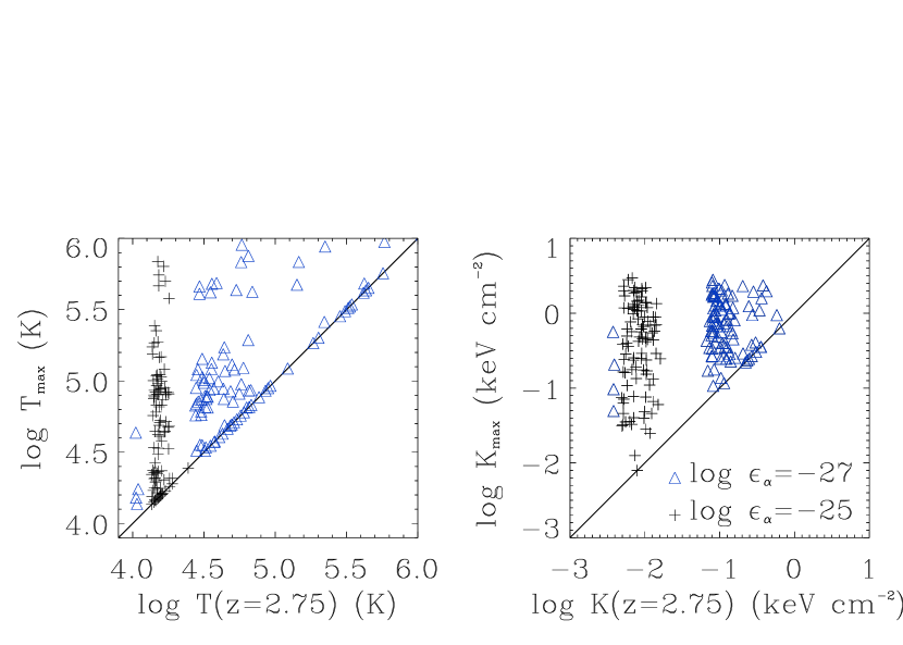
Figure 5.— Left: Compares the current temperature of simulation particles to the maximum temperature achieved in the previous simulation outputs. Since we only have a finite number of outputs, the plotted maximum temperatures are lower limits to the true maxima. We have randomly selected 100 particles from the O3 simulation at $z=2.75$ for each emissivity bin; the triangles and plus signs have $-27.25<\log\epsilon_{\alpha}<-26.75$, and $-25.25<\log\epsilon_{\alpha}<-24.75$, respectively (in units of erg cm^-3 s^-1). The latter bin is composed of self-shielded particles (for which we assume CIE). Right: Same, but for the entropy.

In summary, we cannot neglect the ionizing background (and any additional contribution from local sources) when computing the Ly$\alpha$ emission from the IGM. Unfortunately, its precise role depends on self-shielding and local radiation sources, so a self-consistent treatment will require radiative transfer in full cosmological simulations, including its dynamical effects. Haiman et al. (2000) and Fardal et al. (2001) neglected the ionizing background and argued that the gas would contract after being shocked and radiate its gravitational energy. Instead, we find that the gas settles into a quasistatic phase where photoheating nearly balances radiative cooling. This heat exchange becomes unphysical if (at some point during the contraction) the gas becomes self-shielded (see §3.2). The density at which this transition occurs will determine how much energy the metagalactic ionizing background supplies compared to gravitational collapse (and winds).

4.3. Winds

Most of the simulations that we study include a galactic wind mechanism (see Springel & Hernquist 2003a; Furlanetto et al. 2004a for detailed descriptions of the wind implementation). We might expect this prescription to have important consequences for the Ly$\alpha$ emission. We have therefore also examined some lower resolution runs with weak or no winds (P3 and O3, respectively). In this section we review the effects of the wind prescription on the simulation particles.

The most important consequence of winds is to sharply reduce the star formation rate: the SFR density is $(1.18,0.855,0.244)h^{3}M_{\odot}\,{\rm yr}^{-1}\,\mbox{ Mpc}^{-3}$ at $z=3$ in the (O3, P3, Q3) simulations, bringing the Q3 simulation into reasonable agreement with observations (Springel & Hernquist, 2003b; Hernquist & Springel, 2003). The winds accomplish this in two ways. First, in the absence of ongoing accretion, they simply deplete the gas in the star-forming phase by ejecting it into the IGM. Second, winds interact with gas currently accreting onto halos. In small galaxies, a wind can severely reduce the accretion rates by entraining gas and transporting it out of the halo or by shedding its energy to gas in the outskirts of the halo. In large galaxies, on the other hand, winds remain bound to the halo and only weakly affect the accretion rate. The halo gas rids itself of any wind energy through cooling. In this case even the wind material itself can re-enter the star forming phase after a short delay.

Thus, winds have a substantial effect on gas lying along the cooling locus. In their absence, nearly all of this gas is pristine (i.e., has not formed stars in the past). If we trace the evolution of individual particles, they slowly cool as their densities increase until they are able to form stars. If we turn on weak winds (i.e., those that are unable to escape the gravitational potential wells of typical galaxies), we would expect more gas to lie on the cooling locus because winds eject star-forming particles into the halo and provide extra heat to the accreting gas. Moreover, a significant fraction of the dense gas would have formed stars in the past and thus be metal-enriched. As the winds strengthen, the amount of cool gas should decrease again once they can completely eject particles from galaxy halos. However, some fraction of the wind particles will still be trapped along “accretion channels” and fall back on the galaxies.

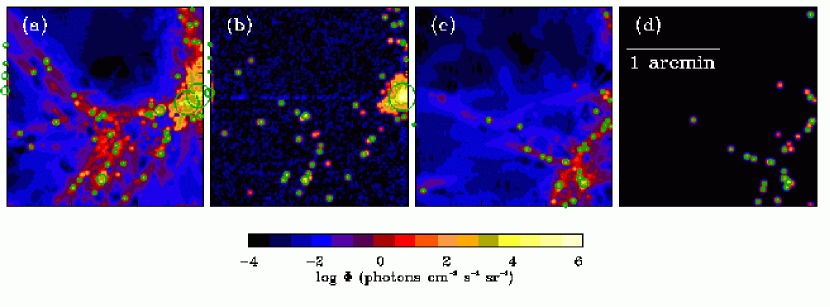
Figure 6.— Maps of Ly$\alpha$ emission from the IGM (a and c), assuming self-shielded gas is in CIE, and from star formation (b and d). All are from the Q5 simulation at $z=3$. Sources identified by SExtractor (with the threshold at $\Phi=100\mbox{ photons s${}^{-1}$ cm${}^{-2}$ sr${}^{-1}$}$ or $9.6\times 10^{-21}\mbox{ erg s${}^{-1}$ cm${}^{-2}$ arcsec${}^{-2}$}$) are outlined in green, with the size proportional to the source’s area on the sky. The slice shown in panels (a) and (b) is unusually rich; the other is more typical. The field is $2.75h^{-1}\mbox{ Mpc}$ wide and $0.67h^{-1}\mbox{ Mpc}$ thick (comoving; this corresponds to 1.2 Å). The angular resolution is $1\arcsec$.

We find precisely this trend in the simulations: the O3 simulation actually has the least amount of gas along the cooling locus, even though it has the highest SFR. The Q3 simulation has slightly more gas in this phase, while the P3 simulation has the most (apparently these weak winds get trapped near the galaxies). In both the Q3 and P3 simulations, a significant fraction of high density, low temperature particles have formed stars in the relatively recent past. Thus winds have complex, and not always intuitive, implications for Ly$\alpha$ emission. However, the effect on the fraction of gas lying along the cooling locus is modest, varying by only a small amount. The upper left part of Figure 2c appears essentially unchanged between the different wind prescriptions.

A more obvious effect is on the shocked, diffuse IGM at high redshifts: without winds, this phase would be considerably weaker in Figure 2c. Of course, current cosmological simulations cannot fully resolve the internal structure of galactic winds. In the nearby universe, winds are observed to have complex multiphase media, including a hot diffuse interior, dense warm clouds, and (in some cases) a cool dense shell of entrained matter. These components are largely unresolved in our simulations and could strongly increase the Ly$\alpha$ luminosity of the wind region and render its geometry more accessible to observations. The true effect of winds may thus be more complex than simply adding gas to the hot, low-density phase.

Winds are clearly complex phenomena, and their effects on Ly$\alpha$ emission are difficult to predict a priori. It is obvious from Figure 2c that the additional hot gas will make a negligible difference to the emission. We will examine the effects on bright emission from the cooling locus in §5.3 below.

5. Ly$\alpha$ Maps

We will now describe the characteristics of narrowband Ly$\alpha$ maps in our simulations. In this section we will focus on qualitative features and global statistics of the maps. We will discuss the statistical properties of well-localized Ly$\alpha$ emitters in §6. Figure 6 shows two example slices of the universe at $z=3$ (taken from the Q5 simulation). The slice is 1.2 Å thick (corresponding to $\Delta z=10^{-3}$ or $0.67h^{-1}\mbox{ Mpc}$ comoving), and the field of view is $2.1\arcmin$ with angular resolution $1\arcsec$ (these correspond to $2.75h^{-1}\mbox{ Mpc}$ and $21.6h^{-1}\mbox{ kpc}$, both comoving). Unless otherwise specified, all of our $z=3$ maps assume these parameters. Panels (a) and (c) show the emission from IGM gas (assuming that the self-shielded gas is in CIE), while (b) and (d) show that from star-forming particles in the corresponding slices. The green circles outline distinct sources (see §6.2 for details). The slice at right is typical for this redshift; the left slice is among the richest few percent in the simulation.

These maps have a number of generic features. First, bright Ly$\alpha$ emission from the IGM and from SF are highly correlated. It is rare for one to appear without the other; as we have described above, this is because most of the luminous IGM particles are either cooling slowly to form stars or have recently felt the effects of galactic winds. The total luminosity of each region is usually dominated by star-forming particles. However, the IGM emission tends to be distributed on somewhat larger scales than the SF. Most of the emission from these coronae (especially in their cores) comes from gas above the self-shielded threshold. As we will show below, these cores depend sensitively on our assumptions about self-shielded gas. Second, Ly$\alpha$ emission is aligned along the cosmic web of filaments, with low surface brightness emission (from optically thin gas) connecting the coronae of bright emission surrounding galaxies. These properties remain true at all redshifts, though the importance of the coronae varies strongly, as we shall show next.

5.1. Redshift Evolution

Figure 7 shows how the statistical properties of the maps evolve with cosmic time. For each redshift, we show the probability distribution function ${\rm d}n/{\rm d}\ln\Phi$ of pixel surface brightness $\Phi$ computed from 120 slices of the highest resolution simulation available at that redshift. In order to better interpret the physical processes as they evolve, we have held the comoving spatial resolution and slice thickness constant with redshift; note then that the angular resolution and spectral width of the observations differ. (They equal the choices of Figure 6 at $z=3$.) We have assumed CIE for the self-shielded gas, although the choice makes no visible difference to this Figure. At all redshifts, ${\rm d}n/{\rm d}\ln\Phi$ peaks at a relatively small surface brightness characteristic of the median cosmic density. In the highly-ionized low-density IGM, recombinations dominate over collisional excitation (see Fig. 1), so the mean surface brightness can be estimated from the recombination rate (Hogan & Weymann, 1987; Gould & Weinberg, 1996). It is:

$$\frac{{\rm d}\Phi}{{\rm d}\lambda_{\rm obs}} = \frac{\eta\dot{n}_{\rm rec}}{4\pi(1+z)^{3}}\,\frac{{\rm d}r_{\rm phys}}{{\rm d}z}\,\frac{{\rm d}z}{{\rm d}\lambda_{\rm obs}}$$ (3)

$$\approx 3\times 10^{-3}\left(\frac{\Omega_{b}h^{2}}{0.02}\right)^{2}\frac{(1+z)^{2}}{h(z)}$$

$$\times\delta^{2}h^{-1}\mbox{ photons cm${}^{-2}$ s${}^{-1}$ sr${}^{-1}$ \AA${}^{-1}$},$$

where $\eta\approx 0.42$ is the fraction of recombinations that produce a Ly$\alpha$ photon, $\dot{n}_{\rm rec}$ is the recombination rate, $h(z)=H(z)/H_{0},$ and $\delta$ represents the effective overdensity (i.e., the density relative to the cosmic mean) of the observed pixel. Here we have used $\alpha=4.2\times 10^{-13}\ {\rm cm}^{3}\ {\rm s}^{-1}$ for the (case-A) recombination rate, appropriate for gas with $T=10^{4}\mbox{ K}$. (This estimate does not apply to the bright coronae, which are not necessarily highly ionized and which have broken off from the cosmic expansion.) We see that $\Phi$ increases with redshift because the mean density and recombination rate increase rapidly. This equation yields a reasonable estimate of the peak of ${\rm d}n/{\rm d}\Phi$, although note that the appropriate $\delta$ changes as structure formation progresses.

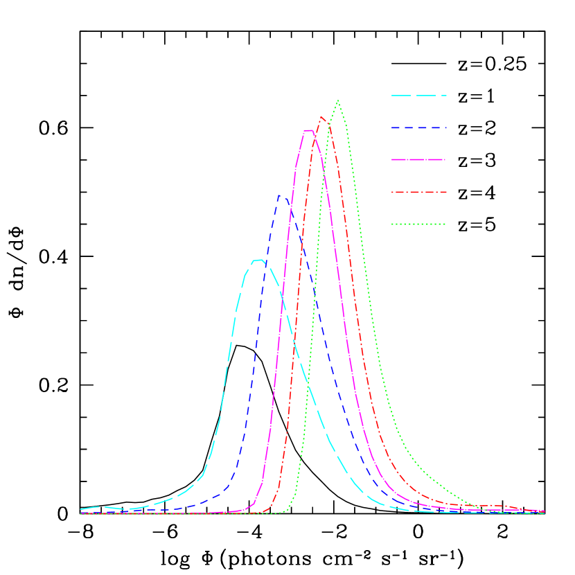
Figure 7.— Evolution of ${\rm d}n/{\rm d}\ln\Phi$. The pixels are $21.6h^{-1}\mbox{ kpc}$ wide and $0.67h^{-1}\mbox{ Mpc}$ thick (comoving); this is $1\arcsec$ wide and 1.2 Å thick at $z=3$. Note that the area under the $z=0.25$ curve is less than unity because $\sim 30\%$ of pixels do not include any simulation particles.

Unfortunately, the probability distributions of the pixel flux peak many orders of magnitude below realistic detection thresholds, regardless of redshift. We therefore focus on the bright end of the distribution in Figure 8, where we show the fraction of pixels above a given threshold surface brightness, $F(>\Phi)$. The first three panels show emission from the IGM if self-shielded gas is in CIE, if it has $\epsilon_{\alpha}=0$, and if it is optically thin to the ionizing background. The fourth shows the total emission from the map (including SF, and assuming CIE for the self-shielded gas).

Looking first at panel (a), we see that the bright pixels evolve in a way that differs qualitatively from the low-density IGM. The brightest emission peaks at $z\sim 2$–$3$ and decreases rapidly toward high and low redshifts. The decline occurs when the cooling locus shifts to low temperatures because the ionizing background is weak and/or soft. As a consequence, $\epsilon_{\alpha}$ declines rapidly if we assume CIE, so the maximum pixel brightness falls. The effect is particularly severe at $z\sim 5$, where the temperature of this component is $T\approx 10^{4.0}\mbox{ K}$ and self-shielded gas is essentially invisible.

Comparison to panel (b), where we set $\epsilon_{\alpha}=0$ for self-shielded gas, shows that nearly all of the emission with $\Phi\gtrsim 100\mbox{ photons s${}^{-1}$ cm${}^{-2}$ sr${}^{-1}$}$ comes from self-shielded gas. If this component cannot emit (either because of strong dust absorption or because the simulation overestimates its temperature), the Ly$\alpha$ coronae become orders of magnitude weaker. Clearly the choice of $n_{\rm ss}$ is crucial in the no emission case. If our prescription is pessimistic (because of embedded sources, for example), the coronae rapidly strengthen. F03 show an explicit example of how the $z=0$ statistics change with the self-shielding cut. Thus observations of diffuse Ly$\alpha$ emission around galaxies can strongly constrain the behavior of cool gas in these environments.

Figure 8c, on the other hand, shows the emission if we assume that all the gas is optically thin to ionizing radiation. Although Schaye (2001a, b) has shown that self-gravitating gas clouds become self-shielded from the metagalactic background at these densities, most of these particles surround star-forming galaxies. As a result, the local ionizing field could be much stronger than the mean, in which case the gas may remain optically thin. In this scenario, the maximum brightness decreases, because optically thin gas is always highly ionized and the CIE collisional excitation peak disappears. However, the fraction of moderately bright pixels remains nearly the same, because the same particles emit (and remain reasonably bright). The exception is at $z=5$, where the optically thin case has much stronger emission. This is because the temperature dependence of $\epsilon_{\alpha}$ is much weaker in the optically thin case, so our predictions are much less sensitive to the location of the cooling locus.

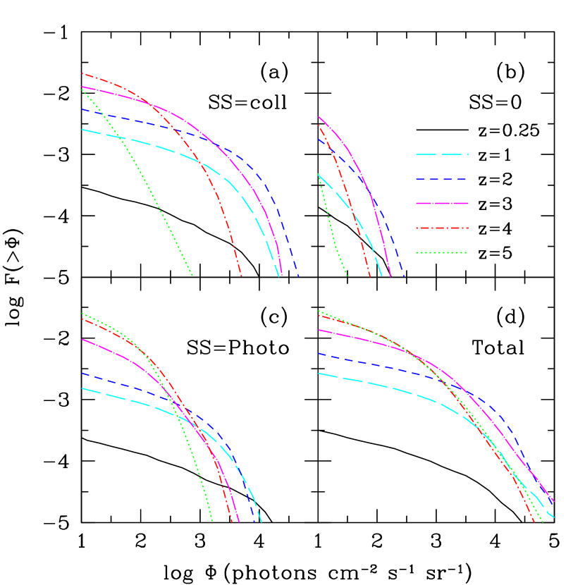
Figure 8.— Evolution of pixel brightness distribution. We show the fraction of pixels above a given surface brightness. The pixels are $21.6h^{-1}\mbox{ kpc}$ wide and $0.67h^{-1}\mbox{ Mpc}$ thick (comoving); this is $1\arcsec$ wide and 1.2 Å thick. (a): IGM emission if self-shielded gas is in CIE. (b): IGM emission without self-shielded gas. (c): IGM emission if all gas is optically thin to ionizing radiation. (d): Total Ly$\alpha$ emission from both the IGM (including self-shielded gas as in panel a) and SF.

The final panel shows that emission due to SF dominates the brightest end of ${\rm d}n/{\rm d}\Phi$ at all redshifts. This is not surprising, as SF produces Ly$\alpha$ photons efficiently. We find that bright emission from SF rises to $z\sim 3$ and then declines slowly at higher redshifts. Although the SFR slowly increases to $z\sim 6$ in these simulations (Springel & Hernquist, 2003b; Hernquist & Springel, 2003), the evolution flattens beyond $z\sim 3$ because the increasing cosmic distance causes the maximum surface brightness to decline. On the other hand, note that the fraction of moderately bright pixels does not change significantly between panels (a) and (d) (except at $z=5$). This is because the IGM Ly$\alpha$ emission is more extended (and fainter) than the star-forming regions, so IGM emission dominates the sky coverage at all but the highest surface brightnesses. Of course, we have assigned all of the Ly$\alpha$ photons from SF to the host particles. Some fraction will actually escape, spreading this component over a wider area. This mechanism will help to boost the IGM emission, even if the ultimate energy source is (photoionization from) SF. Moreover, we have neglected dust absorption, which will likely remove a large fraction ($\gtrsim 75\%$ according to S00) of the SF Ly$\alpha$ photons. Thus the bright tail may not be as pronounced as indicated in Figure 8d and IGM emission (which probably suffers less dust extinction) may be even more important.

Figure 9 shows the redshift evolution in a different way. Here we plot the volume-averaged emissivity in the Ly$\alpha$ line. The solid line shows the total $\epsilon_{\alpha}$ (including both SF and the IGM, assuming CIE for self-shielded gas). The short- and long-dashed curves show $\epsilon_{\alpha}$ from the IGM if we assume CIE for self-shielded gas and that all gas is optically thin, respectively. The dotted curve again shows the total emissivity, but this time in comoving units. We have used the highest resolution simulation available at each redshift to construct the curve; the triangles show estimates from lower resolution simulations with the same parameters. The predictions have converged nicely.

Figure 9.— The evolution of the volume-averaged emissivity $\epsilon_{\alpha}$ in physical units. The solid line shows the total emissivity (assuming CIE for self-shielded gas). The short- and long-dashed curves show $\epsilon_{\alpha}$ from the IGM if we assume CIE for self-shielded gas and that all gas is optically thin, respectively. The dotted line shows the total emissivity per comoving volume. Triangles show the emissivity estimated from lower resolution simulations, while hexagons show it with different wind prescriptions. Filled and open symbols refer to total and IGM emission, respectively.

One of the crucial lessons of Figure 9 is the difference between the two dashed curves. Evidently self-shielded regions dominate the IGM emissivity. The optically thin emissivity closely traces the total (and hence the SFR). Again, this is because $\epsilon_{\alpha}$ depends only weakly on temperature for optically thin gas, so the coronal emission depends (to zeroth order) only on the rate at which galaxies accrete gas (or eject gas through winds), which is itself roughly proportional to the SFR. In contrast, in CIE $\epsilon_{\alpha}$ depends sensitively on temperature. At $z\sim 2$–$3$, quasars make the ionizing background rather hard and intense, so the cooling locus shifts to high temperature and the CIE emissivities are large. But at $z=0$ and $z=5$, the temperatures are small and CIE emissivities fall below the optically thin values. We will focus on $z=3$ in much of the following, and we urge the reader to keep in mind that the CIE assumption is the most optimistic at this epoch.

5.2. Simulation Resolution

We now consider the degree to which the finite simulation resolution affects our results. Figures 10a and 10b show $F(>\Phi)$ for five different simulations at $z=3$. The two panels show results for IGM emission (assuming self-shielded gas is in CIE; other cases yield similar results) and that due to SF, respectively. All the parameters of the slices are the same as in Figure 6. We also use the same number of slices for each simulation. Thus we only sample a small fraction of the volume of the D5 and G6 boxes, and we avoid contamination from rare objects that do not appear in the smaller boxes. The figure shows that our two highest resolution runs, Q4 and Q5, appear to have converged. However, the lower resolution runs (especially G6) show an excess of extremely bright pixels together with a deficit of moderately bright pixels, for both the IGM and star formation. This may seem surprising, because Springel & Hernquist (2003b) showed that the global SFR has converged between all of these simulations. We find deeper convergence problems because we require the spatial distribution of material within halos. In the lower resolution boxes, small halos are not as well-resolved and have SF (and cool gas) confined to only a few particles that fill more compact central regions. Thus the lower resolution simulations can have “cuspier” surface brightness distributions that underestimate the physical extents of the bright Ly$\alpha$ regions. The lower resolution simulations also miss small halos, of course. On the other hand, it is possible that the extra large-scale power in the D5 and G6 simulations genuinely increases the number of bright pixels, by (for example) concentrating the star formation in smaller, highly-biased regions.

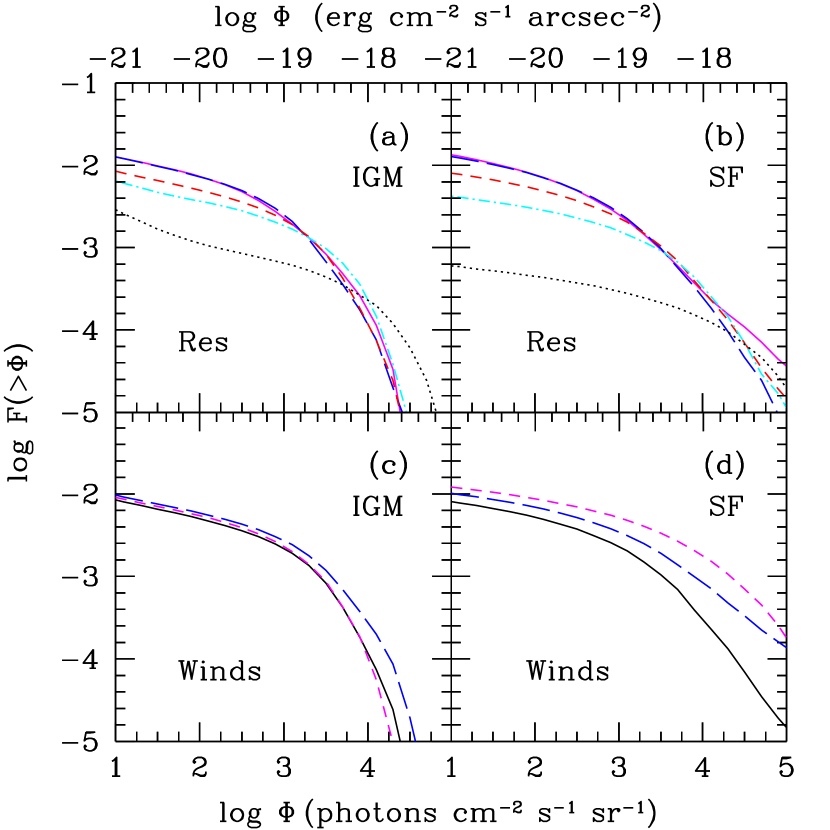
Figure 10.— Bright end of the pixel surface brightness distribution at $z=3$; the pixel scale is the same as in Figure 6. (a): Varying simulation resolution, with self-shielded gas in CIE. The dotted, dot-dashed, short-dashed, long-dashed, and solid curves are for the G6, D5, Q3, Q4, and Q5 simulations, respectively. (b): Same as (a), except for emission from star formation. (c): IGM emission if self-shielded gas is in CIE. The solid, long-dashed, and short-dashed curves have strong, weak, and no winds, respectively. (d): Same as (c), except for emission from SF.

5.3. Winds

As described in §4.3, winds have a substantial impact on the SF properties of the simulation, and we would naively expect them to have comparable effects on the Ly$\alpha$ emission. Figure 10d shows that winds do indeed have substantial implications for the Ly$\alpha$ emission from star-forming particles: the simulations with weak and no winds have nearly an order of magnitude more pixels with $\Phi>10^{4}\mbox{ photons s${}^{-1}$ cm${}^{-2}$ sr${}^{-1}$}$ than the simulation with strong winds. However, Figure 10c shows that the effects on the IGM emission are quite modest. (Here we have assumed CIE for the self-shielded gas, but the differences are small for the other treatments of self-shielded gas as well.) The simulations with strong and no winds have nearly the same $F(>\Phi)$, while weak winds strengthen the emission by only a small amount. This follows the trends expected from the discussion in §4.3, in which we argued that weak winds have the strongest effect on the cooling locus because the winds cannot escape the potential wells of their host galaxies. It is not, however, obvious why the net effect should be so small. It is unclear whether there is a deeper reason for this behavior. We do note that the nature of the bright particles changes between the three simulations. Without winds, the vast majority of the emission comes from particles that have not yet formed stars and contain no metals. With strong winds, fewer than $50\%$ of bright particles are pristine, because a number of formerly star-forming particles have mixed with the gas in the cooling locus.

We also note again that the simulations do not resolve the internal structure of the winds. If the wind medium fragments into dense clumps inside of a more rarefied interclump medium, the total amount of emission could change substantially. The clumps would initially have larger emissivity because of their increased recombination rate; as a result, they would cool more rapidly and could eventually pass below the Ly$\alpha$ excitation threshold. As with self-shielded gas, the resulting emissivity depends sensitively on the equilibrium temperature, which would in turn depend on the ionizing background, continued heat input from the wind, and conduction from the hot intercloud medium. More detailed simulations of individual winds are necessary to resolve these processes.

Figure 9 also compares the volume-averaged $\epsilon_{\alpha}$ across wind simulations. The hexagons show the mean emissivity for the P3 (weak wind) and O3 (no wind) simulations. While the IGM emission is approximately constant in the three cases, the mean SFR rises by a factor of 4–5 from the strong wind case, increasing the total $\epsilon_{\alpha}$ by a large amount.

5.4. Line Widths

We now examine the velocity widths of these Ly$\alpha$ lines. To estimate the distribution, we construct simulation maps as before. For each particle, we also record its velocity (including both the Hubble flow and the peculiar velocity) and velocity dispersion (assuming pure thermal broadening). From these we compute the flux-weighted velocity dispersion $\sigma$ (i.e., the standard deviation of the velocity distribution) of each pixel in the maps, using the same pixel sizes as in Figure 6. Note that $\sigma$ includes thermal broadening, peculiar velocities, and the Hubble flow between particles (but not the Hubble flow gradient within individual particles, because that is negligible for bright, compact particles).

Figure 11 shows the distribution of $\sigma$ per pixel (including IGM emission only, and assuming CIE for the self-shielded component) as a function of surface brightness $\Phi$. Note that the slice has a velocity thickness of $\approx 300\mbox{ km s${}^{-1}$}$; uniform Hubble flow would yield $\sigma\approx 80\mbox{ km s${}^{-1}$}$. This is indeed the peak of the distribution in the low-density IGM.

We see that bright pixels are narrow. Essentially all pixels brighter than 10 photons s^-1 cm^-2 sr^-1 have $\sigma\lesssim 100\mbox{ km s${}^{-1}$}$. At modest brightness ($\sim 100\mbox{ photons s${}^{-1}$ cm${}^{-2}$ sr${}^{-1}$}$), the distribution peaks at $\sigma\approx 10$ to 15 km s^-1, which can be accounted for by thermal broadening at the temperature of the cooling locus. As the brightness increases, the distribution broadens to somewhat larger velocity dispersions, indicating that peculiar motions become relevant. This is probably because the most luminous objects are associated with more massive halos with large internal velocity dispersions (see §6.1). Note, however, that the simulation has only limited resolution for the internal structure of halos, so there may be extra broadening due to rotation, disc formation, etc. Moreover, the coronae should be optically thick to Ly$\alpha$ photons. In this case the photons can only escape by scattering into the wings of the line. Thus the velocities reported here will underestimate the true linewidth. For some geometries, radiative transfer can even change the line’s shape (e.g., Zheng & Miralda-Escudé 2002 and references therein). The best we can say is that the source regions are intrinsically narrow before the effects of radiative transfer have been included.

Figure 11.— The distribution of pixel linewidths $\sigma$ (which we take to be the standard deviation of the line profile), including peculiar velocities and thermal broadening, in the Q5 simulation at $z=3$. We do not include radiative transfer effects. The angular resolution is $1\arcsec$ ($21.6h^{-1}$ comoving kpc) and the slices are 1.2 Å thick ($0.67h^{-1}$ comoving Mpc); $100\mbox{ km s${}^{-1}$}$ corresponds to $0.4$ Å here. The contours are spaced 0.5 dex apart.

5.5. Comparison with the Diffuse Backgrounds

The observability of Ly$\alpha$ emission, especially at the low surface brightness levels relevant for most of the IGM, depends ultimately on the emission strength relative to the diffuse background light. This background can be divided into four components: terrestrial airglow, zodiacal light, diffuse galactic emission (i.e., scattered starlight), and the extragalactic background. The first is obviously unimportant for space-based observations and we will not discuss it further here. The other three are unavoidable.

The best measurements of the backgrounds level in the relevant regime come from Bernstein et al. (2002). They find total backgrounds of $J_{21}\sim 16$–$50$ over the range 3000-8000 Å, where $J_{\nu}=J_{21}\times 10^{-21}\mbox{ erg s${}^{-1}$ cm${}^{-2}$ Hz${}^{-1}$ sr${}^{-1}$}$. Of this total, $\gtrsim 85\%$ comes from the zodiacal light, which can be modeled as reflected sunlight. They estimate that diffuse galactic emission has $J_{21}\sim 0.5$ along clear lines of sight through the Galaxy. The extragalactic background (from galaxies with $V>23$ AB magnitudes) is then $J_{21}=(2.0,1.3,1.1)$ at $(3000,5500,8000)$ Å, with fractional uncertainties of $\sim 50\%$ in each case. These are a few times smaller than the prediction of Haardt & Madau (2001) at $z=0$.

Lines with fluxes above these levels would be straightforward to detect in a background-limited observation. In our units, the integrated background over a velocity width $\Delta v$ is

$$\Phi_{\rm bkgd}=10\,J_{21}\left(\frac{\Delta v}{20\mbox{ km s${}^{-1}$}}\right)\mbox{ photons s${}^{-1}$ cm${}^{-2}$ sr${}^{-1}$}.$$ (4)

As we have seen in §5.4, bright and moderately bright pixels typically have $\sigma\sim 10$–$50\mbox{ km s${}^{-1}$}$, at least if we neglect radiative transfer. Thus we expect that features with $\Phi\gtrsim 100\mbox{ photons s${}^{-1}$ cm${}^{-2}$ sr${}^{-1}$}$ should be visible against the zodiacal light, and features with $\Phi\gtrsim 10\mbox{ photons s${}^{-1}$ cm${}^{-2}$ sr${}^{-1}$}$ should be visible against the other backgrounds. This emphasizes the importance of high spectral resolution observations, because the background increases as the spectral resolution decreases. The typical line widths are $\sim 0.16(\Delta v/20\mbox{ km s${}^{-1}$})[(1+z)/4]$ Å (again neglecting radiative transfer effects). We therefore recommend spectral resolution be a priority in any observations designed to probe the lowest surface brightness objects.

In fact, so long as the background light is either spectrally smooth or can be modeled to high precision, observations can in principle extend far below the limits stated above. For example, spectral features in the zodiacal light mirror those in the solar spectrum and can be modeled fairly well, as Bernstein et al. (2002) did. The Ly$\alpha$ emission would then appear as (weak) fluctuations on the residual background. We emphasize that the background need not be spatially uniform, so long as the spectrum in each pixel is either smooth or can be modeled. Zaldarriaga et al. (2004) discuss in some detail conceptually similar “foreground-cleaning” techniques for low-frequency radio observations (for applications, see also Furlanetto et al. 2004b, c).

6. Source Characteristics

6.1. Luminosity Functions

We will now consider individual Ly$\alpha$ sources. We first divide the simulation particles into gravitationally bound groups using a friends-of-friends group finder with linking length equal to $20\%$ of the mean interparticle separation and a minimum group size of 32 particles. The linking is performed on the dark matter, with each baryonic particle assigned to its nearest dark matter neighbor. We compute the Ly$\alpha$ luminosity of each source as described in §3.

Figure 12 shows some of the characteristics of groups in the Q5 simulation at $z=3$. Panel (a) compares the Ly$\alpha$ luminosity from the IGM to that from SF. The diamonds, triangles, and squares assume self-shielded gas is in CIE, has $\epsilon_{\alpha}=0$, and remains optically thin, respectively. In each case we have randomly selected 300 well-resolved groups to display (i.e., they each have at least 10 times the minimum group mass). The solid line shows $L_{\rm Ly\alpha}=L_{\rm SFR}$. For groups with no ongoing SF, we set $L_{\rm SF}=10^{35}\mbox{ erg s${}^{-1}$}$ if the group has star particles and $L_{\rm SF}=10^{36}\mbox{ erg s${}^{-1}$}$ otherwise. The scatter increases toward lower luminosities, at least in part because accretion and star-formation are more stochastic in halos that are not as well-resolved. Clearly, the SFR and the IGM luminosity are roughly proportional in all treatments, as one would expect if the IGM emission comes from gas that will soon become available for star formation (provided that the gas temperature does not vary strongly between the different groups). The wind prescription also forces the ejected mass to be proportional to the SFR, so it leads to the same relation. $L_{\rm SF}$ typically exceeds the IGM luminosity except in the most optimistic case (which is CIE at $z=3$). The emission from optically thin gas is typically only $\sim 0.01$–$0.05L_{\rm SF}$; if self-shielded gas does not emit, the luminosities of most sources would be completely dominated by the emission from the associated SF. Note, however, that the symbols on the left indicate that some groups have sizable Ly$\alpha$ luminosities even though they are not currently forming stars. Of the groups above our mass threshold, $13\%$ have no ongoing SF but do have star particles, while another $1.7\%$ have neither SF nor star particles.

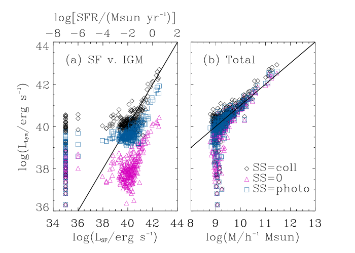
Figure 12.— Characteristics of bound groups in the Q5 simulation at $z=3$. (a): Compares the IGM luminosity to that from stars in each group. If the group has a vanishing current star formation rate (SFR) but contains star particles, we set $L_{\rm SFR}=10^{35}\mbox{ erg s${}^{-1}$}$. If it has no star particles, we set $L_{\rm SFR}=10^{36}\mbox{ erg s${}^{-1}$}$. The solid line shows $L_{\rm SFR}=L_{\rm Ly\alpha,\,IGM}$. (b): Total Ly$\alpha$ luminosity (including SF) as a function of group mass, with the solid line showing the slope if $L_{\rm Ly\alpha}\propto M$. The different sets of points correspond to our different assumptions about self-shielded gas. In each case we have randomly selected 300 well-resolved groups.

Figure 12b shows the total Ly$\alpha$ luminosity as a function of group mass. This is nearly independent of our treatment of self-shielded gas because SF dominates in most cases, except of course for objects without ongoing SF (which are normally near the mass threshold). As we approach this threshold, the scatter increases rapidly because SF is stochastic in poorly-resolved halos. The solid line shows $L_{\rm Ly\alpha}\propto M$. This appears to be slightly too shallow to match the simulations, but only by a small amount. Figure 7 of Springel & Hernquist (2003b) shows that, in the mass range we consider here, the SFR is also roughly proportional to mass, so this is not surprising. For higher mass halos (taken from the D5 simulation, for example), the relation steepens slightly. Interestingly, however, the IGM emission declines slightly relative to that from SF in massive halos. If we had included only IGM emission, $L_{\rm Ly\alpha}\propto M$ remains a reasonable fit, although the relation is slightly steeper if we exclude emission from self-shielded gas.

Figure 13.— The evolution of the luminosity function of groups. (a): Total luminosity function, including both IGM (assuming CIE for self-shielded gas) and SF. (b): IGM emission only, assuming CIE for self-shielded gas. (c): IGM emission only, assuming all gas is optically thin. (d): IGM emission only, assuming $\epsilon_{\alpha}=0$ for self-shielded gas. All distances are comoving. Error bars (shown only for $z=3$) are Poissonian.

This contrasts with the predictions of Haiman et al. (2000) and Fardal et al. (2001), who argue that cooling following gravitational collapse should yield a total luminosity proportional to the binding energy of the halo, or $L_{\rm IGM}\propto M^{5/3}$. We find that the photoionizing background actually provides most of the energy in our calculations; previous work had neglected this component. In this case, the Ly$\alpha$ luminosity should depend primarily on the mass of cool gas in each group, so we naturally expect $L_{\rm Ly\alpha}\propto M$. The fraction of energy that can be traced to the ionizing background is smallest if $\epsilon_{\alpha}=0$ for self-shielded gas, which explains why the relation is steepest in that case. Of course, some of this energy exchange is unphysical, depending on if and when the gas becomes self-shielded (see §4.2). If most of the contraction occurs while gas is shielded, the only available heat source would be gravitational and we would expect $L_{\rm Ly\alpha}\propto M^{5/3}$. The difference could also be due to our wind prescription. Winds eject gas more efficiently in smaller halos and provide a new source (beyond accretion) for the emitting particles. However, although decreasing the strength of the winds increases $L_{\rm SF}$ by a factor of a few, it has little effect on the IGM emission. The IGM luminosity of small groups increases slightly for the weak wind case, but it does not appear to be statistically significant.

Figure 13 shows how the comoving luminosity function of these groups evolves with redshift. Panel (a) shows the total Ly$\alpha$ luminosity of each group, while the others include only IGM emission. Figures 13a and 13b assume that the self-shielded gas is in CIE, Figure 13c assumes that all gas is optically thin, and Figure 13d sets $\epsilon_{\alpha}=0$ for self-shielded gas. We use the Q5 simulation for $z=5$, the D5 simulation for $z=3$ and $2$, and the G5 simulation for $z=0$. We show sample error bars for the D5 simulation at $z=3$ assuming Poisson statistics. Note that the sharp cutoffs at large luminosities for the $z\geq 2$ simulations are not real; they are due to the finite size of the simulation boxes. (However, the difference across panels in the location of the cutoff is real.) The turnover at small luminosity for $z\leq 3$ is due to the finite mass resolution and is also not real.

The trends with redshift are essentially as expected. As emphasized above, the total emission is dominated by SF, so panel (a) qualitatively resembles the “SF multiplicity function” of Springel & Hernquist (2003b) (except that we have not divided low-redshift groups and clusters into their constituent galaxies). In particular, ${\rm d}n/{\rm d}\ln L$ declines at $z\lesssim 1$ along with the global SFR (Springel & Hernquist, 2003b). The IGM luminosity functions depend principally on the treatment of self-shielded gas. Groups at $z\sim 2$–$4$ are most luminous if we assume CIE, while those at $z\sim 0$ and $z\sim 5$ are most luminous if all gas is optically thin. As before, this is a direct consequence of the temperature of the cooling locus. The maximum IGM luminosities without self-shielded gas are much smaller. If this were the most accurate model then it would be considerably more difficult to detect the coronae in Ly$\alpha$ emission.

Figure 14 shows the luminosity function at $z=3$ in several different simulations. Here we show the cumulative function for comparison with existing observations (see §6.3). Panel (a) again shows the total Ly$\alpha$ luminosity of each group, while panel (b) includes only the IGM emission. In both cases we assume that the self-shielded gas is in CIE. These show clearly that our luminosity functions have converged over most of the appropriate range and that the low and high $L_{\rm Ly\alpha}$ cutoffs are not physical. We find similar behavior for the other treatments of dense gas.

As in §5, we find that the IGM emission depends sensitively on our assumptions about dense gas: the luminosity function of this component varies by several orders of magnitude in the different cases. Thus observations of (or constraints on) the diffuse emission around galaxies will help to determine how gas accretes onto galaxies and how this gas interacts with the ionizing background (diffuse and local) and with galactic winds. Like Fardal et al. (2001), we find that the Ly$\alpha$ emission from SF typically dominates the total luminosity, even in the most optimistic IGM treatments. However, the disparity between the two components is not as large as Fardal et al. (2001) claim unless $\epsilon_{\alpha}=0$ for self-shielded gas (see their Figure 2). One possible explanation is that the conservative formulation of SPH employed in our simulations is much less susceptible to numerical overcooling problems that troubled earlier work (Springel & Hernquist, 2002). Another is that Fardal et al. (2001) used a simulation without a photoionizing background to compute the IGM emission. We have argued that this is not a good assumption in general, although it may be adequate if the gas becomes self-shielded before most of the gravitational heating. In that limit their method is in principle a cleaner test of the importance of gravitational shock-heating. Their results lay between our three cases, suggesting that (1) a substantial fraction of the gravitational energy is radiated after the gas becomes self-shielded and/or (2) more of the gravitational energy is radiated through other cooling mechanisms in our simulations. The former is not inconsistent with our results, because the self-shielded gas has contracted more than the optically thin component, which lies in the outskirts of the coronae. We also note that SF emission is much more likely to suffer from dust extinction, which would make the IGM emission easier to see along those lines of sight.

Figure 14.— The Ly$\alpha$ luminosity function of groups at $z=3$ in the different simulations. (a): Total luminosity function, including both IGM (assuming CIE) and SF. (b): Luminosity function for IGM emission only, assuming CIE. All distances are comoving. Error bars are Poissonian.

6.2. Characteristic Sizes

We use SExtractor (version 2.3.2, Bertin & Arnouts 1996) to identify sources within our maps. We choose the default parameter values with the following exceptions: (1) we set the deblending parameter to 0.05 to match the choice of M04, (2) we do not convolve the image with a filter before identifying sources, and (3) we identify sources using an absolute surface brightness rather than a multiple of the local background. We make this choice because our maps are (by construction) background-free and we wish to avoid any artifacts from imposing one.

To give some intuition, the green circles in Figure 6 outline sources identified by SExtractor with a threshold of $\Phi=100\mbox{ photons s${}^{-1}$ cm${}^{-2}$ sr${}^{-1}$}$ (or $9.6\times 10^{-21}\mbox{ erg s${}^{-1}$ cm${}^{-2}$ arcsec${}^{-2}$}$). In each case, the area of the circle is proportional to the isophotal area of the object (though we do not outline the shape of the individual sources). We have set the minimum area to 2 square arcseconds for completeness here. The largest source in the left slice has $A=237$ square arcseconds for SF. It splits into two sources for the IGM, with $A=185$ and 182 square arcseconds. Only five (or three) other sources have $A>10$ square arcseconds for IGM (or SF). In the right-hand map, only two sources have $A>10$ square arcseconds, in both IGM and SF. In general, the IGM Ly$\alpha$ emission is more spatially extended but fainter than the associated emission from SF.

Figure 15 shows a scatter plot of isophotal area versus mean surface brightness for slices from the Q5 simulation at $z=3$. We have used ten slices of thickness $\Delta z=0.01$ and width $5.5h^{-1}\mbox{ Mpc}$ (comoving) to construct the sample. The angular resolution is $1\arcsec$ (equal to $21.6h^{-1}$ comoving kpc). The total volume is thus about twice the volume of the Q5 box (but most repeated sources will be viewed from different directions). In all cases we have imposed a minimum source area of 5 square arcseconds. The triangles are for SF, while the other symbols show the IGM emission for our three cases. Figures 15a and b have detection thresholds of $\Phi=7000\mbox{ photons s${}^{-1}$ cm${}^{-2}$ sr${}^{-1}$}$ (or $6.7\times 10^{-19}\mbox{ erg s${}^{-1}$ cm${}^{-2}$ arcsec${}^{-2}$}$) and $\Phi=100\mbox{ photons s${}^{-1}$ cm${}^{-2}$ sr${}^{-1}$}$ (or $9.6\times 10^{-21}\mbox{ erg s${}^{-1}$ cm${}^{-2}$ arcsec${}^{-2}$}$), respectively. For the former, there are no IGM emitters that meet this threshold unless the self-shielded gas is in CIE; the other samples are complete. For the lower threshold of Figure 15b, we randomly select 250 objects from the samples (unless $\epsilon_{\alpha}=0$ for self-shielded gas, in which case only 16 sources meet our criteria).

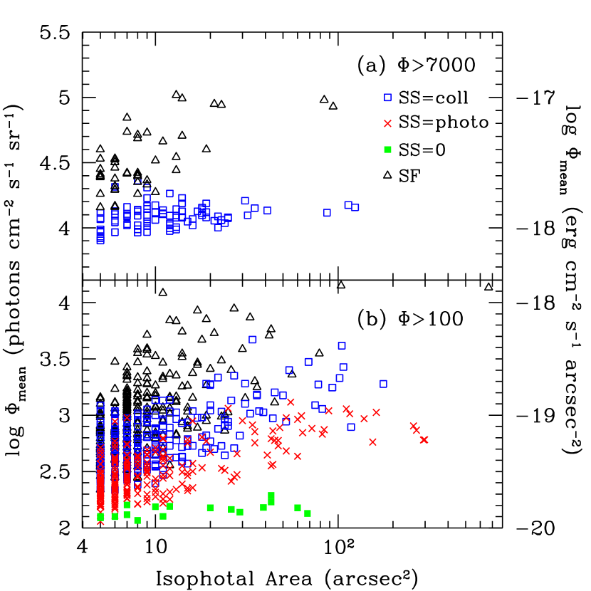
Figure 15.— Scatter plot of angular size against mean surface brightness for sources from the Q5 simulation at $z=3$. Panels (a) and (b) have $\Phi=7000$ and $100\mbox{ photons s${}^{-1}$ cm${}^{-2}$ sr${}^{-1}$}$ (or $6.7\times 10^{-19}$ and $9.6\times 10^{-21}\mbox{ erg s${}^{-1}$ cm${}^{-2}$ arcsec${}^{-2}$}$), respectively. The triangles are for emission from SF; other symbols are for IGM emission with the different treatments of self-shielded gas. Note that $1\arcsec=21.6h^{-1}$ comoving kpc.

Comparing the IGM and SF points at the two $\Phi$ thresholds, we see that the IGM emission is usually fainter but more extended than the SF component. This remains true until the highest thresholds, when the IGM emission cuts off before SF emission; of course the location of the cutoff depends on the treatment of dense gas. At the flux levels currently accessible to observations (Figure 15a) IGM emission will be difficult to detect except where it is self-shielded, has a high temperature, and is in CIE. Interestingly, in this case there are about twice as many IGM sources with $\Phi>7000\mbox{ photons s${}^{-1}$ cm${}^{-2}$ sr${}^{-1}$}$ as there are SF sources; this is because most of the star-forming regions have $A<5$ square arcseconds.

Figures 16 and 17 show the source characteristics in a more quantitative form. Figure 16 shows the angular density of Ly$\alpha$ sources per unit redshift as a function of isophotal area (note that the cutoff at small area is a result of the minimum detection area we set in SExtractor). Panel (a) compares the total (including SF and assuming CIE for self-shielded gas, solid curve) and IGM (dashed curves for CIE, dot-dashed curve for optically thin gas) emission at two different flux thresholds, $\Phi=10^{3}$ and $2.3\times 10^{4}\mbox{ photons s${}^{-1}$ cm${}^{-2}$ sr${}^{-1}$}$ (or $9.6\times 10^{-20}$ and $2.2\times 10^{-18}\mbox{ erg s${}^{-1}$ cm${}^{-2}$ arcsec${}^{-2}$}$; thick and thin curves, respectively). Note that there are no objects with $\Phi>2.3\times 10^{4}\mbox{ photons s${}^{-1}$ cm${}^{-2}$ sr${}^{-1}$}$ if all gas is optically thin. Again, we find that the isophotal area of the total emission is dominated by the IGM at small $\Phi$, but at sufficiently large surface brightness thresholds, the SF component dominates by a large factor.

Figure 16b shows the total emission for the Q5 (solid), D5 (dashed), and G6 (dotted) simulations. We also show error bars on the Q5 curve, assuming Poisson statistics. Clearly the G6 simulation underestimates both the number of faint, compact sources and the number of highly extended sources. The former occurs because the simulations have a finite mass resolution. The latter probably occurs because the larger-scale simulations do not fully resolve the spatial distribution of SF within halos, even though the global SFR converges (see §5.2). The higher-resolution simulations do seem to have converged reasonably well.

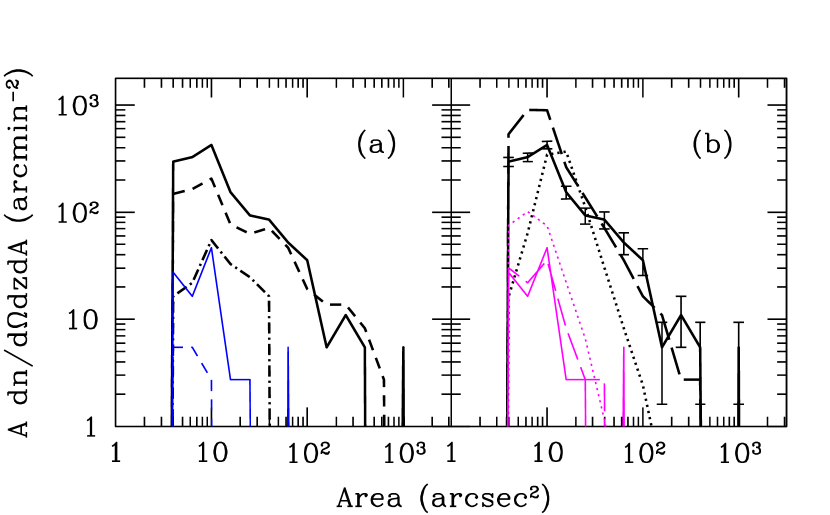
Figure 16.— The distribution of Ly$\alpha$ emitters as a function of isophotal area at $z=3$. The angular resolution is $1\arcsec$ ($21.6h^{-1}$ comoving kpc). (a): The solid curves show total emission, while the dashed and dot-dashed curves show emission from the IGM only, assuming CIE for self-shielded gas and that all gas is optically thin, respectively. Thick and thin curves set the threshold at $\Phi=10^{3}$ and $2.3\times 10^{4}\mbox{ photons s${}^{-1}$ cm${}^{-2}$ sr${}^{-1}$}$ (or $9.6\times 10^{-20}$ and $2.2\times 10^{-18}\mbox{ erg s${}^{-1}$ cm${}^{-2}$ arcsec${}^{-2}$}$). All curves are from the Q5 simulation. (b): The solid, dashed, and dotted curves are for total (IGM and star formation) emission in the Q5, D5, and G6 simulations. The cutoff at small area is due to the SExtractor threshold that we chose.

Figure 17 shows similar information, except as a function of the mean surface brightness. Panel (a) shows that the SF component dominates the total brightness, especially if the dense gas is optically thin (or if it cannot emit). Note also that a larger area threshold decreases the abundance of both faint and extremely bright sources. Figure 17b shows poor convergence in the brightness distribution: the number of sources with $\Phi>10^{4}\mbox{ photons s${}^{-1}$ cm${}^{-2}$ sr${}^{-1}$}$ varies by more than an order of magnitude between the simulations. This may be surprising given that the Ly$\alpha$ luminosity function converges reasonably well. It is again a result of failing to resolve the spatial distribution of the gas. The high-resolution simulations better describe the extended, cool gas, so the sources have larger areas and hence smaller mean $\Phi$ (even for the same intrinsic luminosity).

We note that winds have little effect on the sizes of the Ly$\alpha$ emitters. There is weak evidence that the low surface brightness IGM emission is slightly more extended in the case of strong winds, but it is not a significant difference. This is not surprising given that the winds will have difficulty escaping along the direction of bright, dense particles.

In this section we have focused on $z=3$, because that is where the most complete observations are. However, our qualitative conclusions hold at other redshifts as well: star-forming regions produce compact, bright Ly$\alpha$ emission surrounded by extended, fainter IGM emission.

6.3. Comparison to Observations

In the past several years, Ly$\alpha$ line selection has become an increasingly popular technique to identify high-redshift objects. The usual procedure is to compare broadband and narrowband images of a field; those objects that have high equivalent widths in the narrowband image are likely to be emission-line galaxies. In most cases, contamination from other lines (particularly [O II] $\lambda 3727$ at low redshifts) is a worry, but color selection and spectroscopic follow-up can determine the sample purity. To date, most studies have focused on relatively high-surface brightness emission from star-forming galaxies.

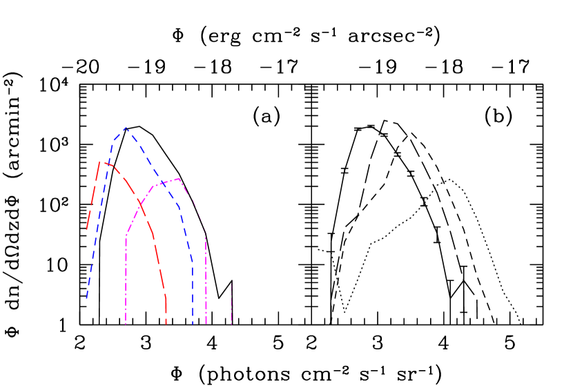
Figure 17.— The distribution of Ly$\alpha$ emitters as a function of mean surface brightness at $z=3$. The angular resolution is $1\arcsec$ ($21.6h^{-1}$ comoving kpc). (a): The solid, short-dashed, and long-dashed lines are for the total emission, IGM assuming CIE for self-shielded gas, and IGM assuming that all gas is optically thin; each of these has $A_{\rm min}=5$ square arcseconds. The dot-dashed line shows the total emission with $A_{\rm min}=16$ square arcseconds. (b): The solid, long-dashed, short-dashed, and dotted curves are for total emission in the Q5, Q3, D5, and G6 simulations, with $A_{\rm min}=5$ square arcseconds.

A number of these surveys have constrained the space density of luminous, relatively compact Ly$\alpha$ emitters. We will begin by comparing these observations to our results. Cowie & Hu (1998) performed blank-field surveys at $z\approx 3.4$ and found $n\sim(3,1)\times 10^{-3}h^{3}\mbox{ Mpc${}^{-3}$}$ for objects with $L_{42}\gtrsim(2,5)$. Here $L_{\rm Ly\alpha}=L_{42}\times 10^{42}\mbox{ erg s${}^{-1}$}$. This is about an order of magnitude smaller than the predictions of Figure 14. (Note that the luminosity function evolves only weakly with redshift in the range $z\sim 2$–$5$.) S00 found a space density about 6 times larger than Cowie & Hu (1998); however, the S00 volume contains $\sim 6$ times as many continuum-selected galaxies as an average field, so this is probably due to cosmic variance. Fujita et al. (2003) find $n\sim 2\times 10^{-4}h^{3}\mbox{ Mpc${}^{-3}$}$ for objects with $L_{42}\gtrsim 5$ at $z=3.7$, several times smaller than Cowie & Hu (1998). Ouchi et al. (2003) performed a survey for Ly$\alpha$ emitters at $z=4.86$ and found no evidence for evolution in the luminosity function between that time and $z=3.4$. Palunas et al. (2004) found $n\sim 3\times 10^{-4}h^{3}\mbox{ Mpc${}^{-3}$}$ for $L_{42}\gtrsim 4$ at $z=2.38$, also consistent with weak redshift evolution.

All of these surveys have different selection criteria, so detailed comparisons to our luminosity function are difficult. However, it seems clear that our predictions are roughly an order of magnitude above the observed number densities at $L_{42}\sim 1$–$10$. There are several possible explanations for the discrepancy. First, we have included the total emission from SF and the IGM. The IGM emission is relatively extended and may not actually contribute to the observed high-surface brightness emission. If the CIE case is overly optimistic, this would also decrease the luminosities by about $50\%$. Second, we have ignored processes within the galaxies that can dramatically modify the Ly$\alpha$ line luminosity, such as dust (which appears to completely eliminate or substantially reduce Ly$\alpha$ emission in $\sim 75$–$80\%$ of $z=3$ galaxies; S00, Shapley et al. 2003). Such a correction would bring our estimates into reasonable agreement with most of the observations described above. The dust extinction probably depends on the line of sight through the galaxy (and its wind); much of the galaxy will therefore show little Ly$\alpha$ emission, allowing the IGM to stand out more clearly. Third, we have used a crude conversion of SFR to $L_{\rm Ly\alpha}$ (see §3.3). A more sophisticated treatment may help to reconcile the predictions with the observed number density.

To probe the IGM emission, it is best to consider extended objects with relatively low surface brightness. S00 and M04 have detected extended “blobs” of Ly$\alpha$ emission without associated (significant) UV continua near a “proto-cluster” of Lyman-break galaxies. S00 detected two blobs with $L_{\rm Ly\alpha}\sim 10^{44}\mbox{ erg s${}^{-1}$}$ and physical extents of $\sim 100h^{-1}\mbox{ kpc}$, implying $n\sim 3\times 10^{-4}h^{3}\mbox{ Mpc${}^{-3}$}$ for these objects. (Note, however, that this is the same field cited above and has $\sim 6$ times as many galaxies as average). M04 surveyed an overlapping field (with effective volume about eight times larger) and selected objects with $A>16$ square arcseconds and $\Phi\gtrsim 2.3\times 10^{4}\mbox{ photons s${}^{-1}$ cm${}^{-2}$ sr${}^{-1}$}$ ($2.2\times 10^{-18}\mbox{ erg s${}^{-1}$ cm${}^{-2}$ arcsec${}^{-2}$}$); they find $n\sim 7\times 10^{-4}h^{3}\mbox{ Mpc${}^{-3}$}$. These objects have $L_{42}\gtrsim 6$.

Extended emission is thus somewhat rarer than the compact Ly$\alpha$ emitters probed by most surveys, and our models can easily accommodate the raw luminosities of the M04 sample. Figure 14b shows that the IGM component on its own can provide enough energy so long as we assume CIE. However, most of the sources in the simulation are much smaller than the M04 objects. With their area and surface brightness thresholds, we find $n_{\rm sim}\sim(3,20)\times 10^{-4}h^{3}\mbox{ Mpc${}^{-3}$}$ for IGM and total emission, respectively, assuming CIE for self-shielded gas. In the other cases no IGM objects satisfy these criteria. Unfortunately, these predictions are based on only a few objects and have not fully converged for the IGM emission. The strongest statement we can make is that star formation appears to produce easily enough Ly$\alpha$ emission on moderately large ($A\sim 20$–$40$ square arcsecond) scales to explain the observations, even if we renormalize the number densities to match that of Ly$\alpha$ galaxies (thus crudely accounting for dust extinction in the SF component). However, the IGM on its own could only account for the blobs in the most optimistic case.

If we consider the most luminous and most extended objects, the IGM looks to be even less plausible. At the M04 $\Phi$ threshold, none of our objects have $A>60$ square arcseconds even if we include star formation, while $\sim 10\%$ of the observed blobs exceed this size (and the largest has $A=222$ square arcseconds). We most likely therefore need to appeal to other processes to explain the largest and most luminous blobs (including those first discovered by S00), although we cannot rule out that the finite size of our simulation box is responsible for the difference. We must also stress that the observed luminous Ly$\alpha$ blobs have velocity widths of several hundred km s^-1 (S00; Bower et al. 2004), much larger than the intrinsic widths of our sources (see §5.4). If these sources are ultimately due to cooling gas and SF, large internal velocity gradients (from winds, for example) or complex radiative transfer (e.g., Zheng & Miralda-Escudé 2002) would have to dramatically alter our predicted linewidths. On the other hand, both S00 and M04 selected a region known to contain a strong galaxy overdensity, and the density of blobs in more normal environments is unknown. M04 note that the blobs are highly clustered even within their region. Observations of more representative regions would be invaluable in understanding the nature of strong Ly$\alpha$ emission.

Another interesting issue is the correlation between IGM emitters and galaxies. In our simulations, Ly$\alpha$ sources without associated stellar particles are extremely rare. In most cases, those that do exist are associated with poorly-resolved halos and may be simulation artifacts. Thus, within the context of our simulations, isolated bright Ly$\alpha$ emitters will be rare. Although the luminous S00 blobs are not centered on optically visible galaxies, at least one of them has a vigorously star-forming (SFR $\gtrsim 500h^{-2}\mbox{ M${}_{\odot}$ yr${}^{-1}$}$) submm galaxy near its center (Chapman et al., 2001) and both have optical galaxies near their outskirts. M04 found that 7/33 other blobs match with previously detected galaxies. The others may also be associated with faint galaxies (perhaps due to intrinsic absorption), and testing this connection would be useful in the future. Such observations could also help to measure the relative importance of Ly$\alpha$ from SF and the IGM in different galaxies. We have found that SF usually dominates the total luminosity of each system; however, we have also found that our simulations overestimate the number density of Ly$\alpha$ -emitting galaxies. This is likely due to internal structure and the dust distribution within galaxies. The IGM emission should be less susceptible to these uncertainties, so in some cases it may actually dominate the observed emission.

Finally, we have neglected radiative transfer in computing the source sizes. Because our regions are optically thick in the Ly$\alpha$ line, these photons scatter resonantly until reaching an optical depth near unity. Although most of the scattering occurs in frequency space, some photons could in principle also scatter in real space to the edge of the optically thick region, from which they can escape even from the center of the line. Thus our method may underestimate the true extent of the emitting regions. Fardal et al. (2001) argue that this mechanism can help to reconcile the luminous, compact sources found in their simulations with the significantly more extended observed systems. Furthermore, ionizing photons from young stars in the central galaxy can escape into the surrounding IGM but get absorbed by the cool, dense gas. This would shift some of the Ly$\alpha$ emission that we attribute to star formation into the IGM, making the SF sources larger than we have found.

7. Discussion

We have used cosmological simulations to study the Ly$\alpha$ emission expected from structure formation over a broad range of redshifts. We considered emission from optically thin low-density gas, from self-shielded gas clouds, and from the reprocessing of stellar ionizing photons. As in F03, who studied Ly$\alpha$ emission from $z\lesssim 0.5$, we have found that the brightest regions are compact star-forming galaxies. These are surrounded by extended coronae of emission from IGM gas; the regions closest to galaxies are likely to be self-shielded (at least from the mean ionizing background) while the outer reaches remain optically thin. Crucially, although emission associated with star formation dominates the total Ly$\alpha$ luminosity, the IGM coronae are more extended and can thus be isolated (at least in principle). They could also dominate in galaxies in which dust has extinguished the Ly$\alpha$ line from star formation. However, the luminosities of the coronae depend sensitively on our assumptions about gas that is able to shield itself from the metagalactic ionizing background.

One of the most important results of this study is that the photoionizing background can power the bright Ly$\alpha$ coronae, in contrast to earlier predictions in which gravitational energy dominated (Haiman et al., 2000; Fardal et al., 2001). In our simulations, most of the flux comes from gas on a high density ($n_{\rm H}\gtrsim 10^{-3}\mbox{ cm${}^{-3}$}$), low temperature ($T\lesssim 10^{4.5}\mbox{ K}$) track of particles bound to dark matter halos but outside of galaxies. Although many of these dense particles have been moderately shocked in the past (see Figure 5), the post-shock cooling times are so short that they quickly enter a quasi-equilibrium cool phase. In this regime, photoheating and radiative cooling nearly balance, increasing the cooling time. While it is optically thin, the ionizing background powers $\gtrsim 50\%$ of the Ly$\alpha$ emission at $z\geq 1$, provided that it is near or above our fiducial amplitude. As the gas condenses, we expect it to eventually become self-shielded from the diffuse ionizing background. Because we cannot include radiative transfer in our calculations, the power source beyond this point is unclear. If gravitational contraction or winds maintain the gas temperature near the peak for Ly$\alpha$ excitation, photoionization would play a relatively minor role. If, on the other hand, the dense gas rapidly cools or remains optically thin (in particular due to embedded sources), photoionization can power $\gtrsim 90\%$ of the Ly$\alpha$ emissivity. We thus argue that including photoionizing radiation is crucial to interpreting observations of Ly$\alpha$ cooling around galaxies.

In any of these cases, the cool gas in Ly$\alpha$ coronae directly traces the accretion of gas onto galaxies, although winds do significantly complicate the interpretation. In the presence of winds, Ly$\alpha$ emission comes from a mix of relatively pristine accreting gas and material that has recently been ejected from the central galaxy but remains trapped inside the halo (either because the wind velocity is smaller than the escape speed of the halo, or because the wind interacts with the accreting gas). We find, however, that winds have a surprisingly small effect on the Ly$\alpha$ emission (especially considering that they reduce the global SFR by a factor of five), although our simulations do not fully resolve the winds. Clumping within the wind medium could increase the local emissivity, or the faster cooling may end up reducing the total emission.

Thus the Ly$\alpha$ coronae present the intriguing opportunity to measure some combination of wind feedback near and gas accretion onto galaxies. Unfortunately, the self-shielded gas responsible for most of the emission is also the most difficult to model. We have emphasized several uncertainties in §3.2, including the presence of dust, the geometry and velocity structure of the region, radiative transfer of higher Lyman line photons through the cloud, the temperature of the self-shielded gas, and the local ionizing radiation field. Of these, the last two are likely the most important.

The temperature of gas on the cooling locus is determined in the simulation by the balance between photoheating and radiative cooling. If the cloud is self-shielded, the primary heat source disappears and it may cool rapidly. The Ly$\alpha$ emissivity is extremely sensitive to the temperature in collisionally ionized gas, so small errors in the heat balance could translate into large changes in the emission properties. Unfortunately, the simulations do not include self-shielding because they do not incorporate a self-consistent treatment of radiative transfer. Although we can crudely identify regions that are shielded from the metagalactic ionizing background, we cannot account for radiation from nearby galaxies or self-consistently describe the behavior of shielded gas. We therefore consider three cases that should bracket the real behavior. In the first, we set the emissivity of self-shielded gas to zero, which would be a good approximation if the gas were to cool efficiently. In the second, we assume that the simulation temperatures are accurate and that the self-shielded gas is in CIE. In the third, we assume that the local ionizing field is much larger than the mean, so that even dense gas remains optically thin. In the first case, IGM gas is extremely faint and may be beyond the reach of near-future surveys. But in either of the other cases, the gas is significantly brighter and the total luminosity is not too far below that from star formation. The balance between the two optimistic cases depends on redshift, because the emissivity in CIE is extremely sensitive to temperature, which, in our simulations, is set by the ionizing background.

We have also computed the Ly$\alpha$ emission from recombinations following absorption of stellar ionizing photons inside galaxies. We have used an extremely simple conversion between local SFR and Ly$\alpha$ luminosity (see §3.3), appropriate for a standard IMF and little extinction. The true luminosity will vary with the initial mass function, metallicity, dust content, and internal structure of each galaxy, so our quantitative results should be viewed as no more than representative. With these assumptions, this component dominates both the total luminosity and the brightest pixels, but it is confined to smaller physical scales than the IGM emission. We have, however, assumed that all of the ionizing photons are absorbed locally. In reality, some fraction of the ionizing photons will escape the host galaxy into the surrounding IGM (Steidel et al., 2001; Lequeux et al., 1995; Kunth et al., 2003). It is this radiation that could escape and help to illuminate the nominally self-shielded gas in the Ly$\alpha$ coronae. By neglecting dust, we have also overestimated the total amount of SF Ly$\alpha$ radiation by a factor of $\sim 4$ (at $z=3$; S00). Both of these effects help to increase the relative importance of IGM emission.

A number of recent observations have targeted high-redshift galaxies with strong Ly$\alpha$ emission (see §6.3). The space density of such objects is about an order of magnitude smaller than predicted by our simulations. A large part of this difference is likely because only $\sim 20$–$25\%$ of star-forming galaxies have strong Ly$\alpha$ emission (S00), for the reasons outlined above. The remaining discrepancy is reasonable given the simple assumptions behind our model. Our results therefore suggest that Ly$\alpha$ selection can be a useful probe of galaxy formation and gas accretion, even if high-surface brightness galaxies are the only targets. This is particularly interesting given that Ly$\alpha$ -selection is currently the most efficient technique to select the highest-redshift galaxies (e.g., Hu et al. 2002; Kodaira et al. 2003; Rhoads et al. 2004) and can potentially be a powerful probe at even earlier epochs (Barton et al. 2004; though absorption from the neutral intervening IGM could complicate such an interpretation; see, e.g., Furlanetto et al. 2004d and references therein).

We have emphasized the substantial uncertainties in Ly$\alpha$ emission from both the IGM and star formation. While these imply that our predictions are far from rigorous, they present an excellent opportunity to constrain the models through observations. Existing surveys for diffuse Ly$\alpha$ emission at $z\sim 2$–$3$ have reached surface brightness thresholds of $\sim 2.3\times 10^{4}\mbox{ photons s${}^{-1}$ cm${}^{-2}$ sr${}^{-1}$}$ (or $2.2\times 10^{-18}\mbox{ erg s${}^{-1}$ cm${}^{-2}$ arcsec${}^{-2}$}$ at $z=3.1$; M04) with the Subaru telescope and $\sim 1.3\times 10^{4}\mbox{ photons s${}^{-1}$ cm${}^{-2}$ sr${}^{-1}$}$ (or $1.6\times 10^{-18}\mbox{ erg s${}^{-1}$ cm${}^{-2}$ arcsec${}^{-2}$}$ at $z=2.2$; Francis & Bland-Hawthorn 2004) with the 4-meter Anglo-Australian Telescope. Both are fairly close to our more optimistic predictions. We have shown that the combination of star formation and cooling gas powered by the photoionizing background can in principle account for most of the Ly$\alpha$ blobs observed by M04, although we found no counterparts to the largest and most luminous blobs identified by S00. IGM emission alone probably cannot explain the observations, but in our more optimistic cases should appear with order-of-magnitude increases in the surface brightness sensitivity.

We find no evidence in our simulations for strong Ly$\alpha$ emission except that surrounding galaxies. We therefore expect that all the Ly$\alpha$ blobs observed at $z\sim 3$ contain embedded galaxies, which could be tested through follow-up observations of the M04 sources. An alternate approach to find isolated emitters is to seek quasar absorption line systems in emission (Hogan & Weymann, 1987). Analytic estimates suggest that optically-thick Lyman-limit systems should be visible through reprocessing of the ionizing background (Gould & Weinberg, 1996). In our simulations, it is most natural to associate these with the Ly$\alpha$ coronae around galaxies, so it is important to identify the absorber environments through observations. Such searches are already underway. Francis & Bland-Hawthorn (2004) searched for diffuse emission near a bright quasar at $z=2.168$. They found no sources with $A>9$ square arcseconds and $\Phi>1.3\times 10^{4}\mbox{ photons s${}^{-1}$ cm${}^{-2}$ sr${}^{-1}$}$. This is somewhat surprising in our model, given that we expect a quasar to be embedded inside an overdensity with an abundance of cool gas; the peak brightness should be at least comparable to their threshold if the gas emits in collisional ionization equilibrium. The most likely explanation is that the quasar has photoionized all of the nominally self-shielded gas. This would reduce the peak to $\Phi\sim 10^{3}$-$10^{4}\mbox{ photons s${}^{-1}$ cm${}^{-2}$ sr${}^{-1}$}$ (see Figure 8c), just below the existing threshold. We therefore argue that it is crucial to continue to push these narrowband observations forward. Francis & Bland-Hawthorn (2004) have demonstrated that valuable upper limits can be obtained even from 4-meter class telescopes, and our results suggest that direct detection of diffuse Ly$\alpha$ emission may not be far away.

References

- Barkana & Loeb (2001) Barkana, R., & Loeb, A. 2001, Phys. Rep., 349, 125
- Barton et al. (2004) Barton, E. J., Davé, R., Smith, J. T., Papovich, C., Hernquist, L., & Springel, V. 2004, ApJ, 604, L1
- Bernstein et al. (2002) Bernstein, R. A., Freedman, W. L., & Madore, B. F. 2002, ApJ, 571, 56
- Bertin & Arnouts (1996) Bertin, E., & Arnouts, S. 1996, A&AS, 117, 393
- Birnboim & Dekel (2003) Birnboim, Y. & Dekel, A. 2003, MNRAS, 345, 349
- Bower et al. (2004) Bower, R. G., et al. 2004, MNRAS, 351, 63
- Cen & Ostriker (1999) Cen, R., & Ostriker, J. P. 1999, ApJ, 514, 1
- Chapman et al. (2001) Chapman, S. C., et al. 2001, ApJ, 548, L17
- Cowie & Hu (1998) Cowie, L. L. & Hu, E. M. 1998, AJ, 115, 1319
- Croft et al. (2002) Croft, R. A. C., et al. 2002, ApJ, 581, 20
- Davé et al. (2001) Davé, R., et al. 2001, ApJ, 552, 473
- Fardal et al. (2001) Fardal, M. A., et al. 2001, ApJ, 562, 605
- Ferland (2003) Ferland, G. J. 2003, Hazy, A Brief Introduction to Cloudy 96.00 (http://www.nublado.org/)
- Francis & Bland-Hawthorn (2004) Francis, P. J., & Bland-Hawthorn, J. 2004, MNRAS, in press, (astro-ph/0405506)
- Fujita et al. (2003) Fujita, S. S., et al. 2003, AJ, 125, 13
- Furlanetto & Loeb (2004) Furlanetto, S. R., & Loeb, A. 2004, ApJ, 611, 642
- Furlanetto et al. (2003) Furlanetto, S. R., Schaye, J., Springel, V., & Hernquist, L. 2003, ApJ, 599, L1 (F03)
- Furlanetto et al. (2004a) —. 2004a, ApJ, 606, 221
- Furlanetto et al. (2004b) Furlanetto, S. R., Zaldarriaga, M., & Hernquist, L. 2004b, ApJ, 613, 1
- Furlanetto et al. (2004c) Furlanetto, S. R., Zaldarriaga, M., & Hernquist, L. 2004c, ApJ, 613, 16
- Furlanetto et al. (2004d) Furlanetto, S. R., Hernquist, L., & Zaldarriaga, M. 2004d, MNRAS, in press, (astro-ph/0406131)
- Fynbo et al. (1999) Fynbo, J. U., Møller, P., & Warren, S. J. 1999, MNRAS, 305, 849
- Fynbo et al. (2000) Fynbo, J. U., Thomsen, B., & Möller, P. 2000, A&A, 353, 457
- Gould & Weinberg (1996) Gould, A., & Weinberg, D. H. 1996, ApJ, 468, 462
- Haardt & Madau (1996) Haardt, F. & Madau, P. 1996, ApJ, 461, 20
- Haardt & Madau (2001) Haardt, F., & Madau, P. 2001, in Clusters of Galaxies and the High Redshift Universe Observed in X-rays, ed. D. M. Neumann & J. T. T. Van (21st Moriond Astrophysics Meeting, Les Arc, France)
- Haiman et al. (2000) Haiman, Z., Spaans, M., & Quataert, E. 2000, ApJ, 537, L5
- Hernquist & Springel (2003) Hernquist, L. & Springel, V. 2003, MNRAS, 341, 1253
- Hogan & Weymann (1987) Hogan, C. J., & Weymann, R. J. 1987, MNRAS, 225, 1P
- Hu et al. (2002) Hu, E. M., et al. 2002, ApJ, 568, L75
- Hui & Gnedin (1997) Hui, L., & Gnedin, N. Y. 1997, MNRAS, 292, 27
- Katz et al. (1996a) Katz, N., Weinberg, D. H., Hernquist, L., & Miralda-Escudé, J. 1996a, ApJ, 457, L57
- Katz et al. (1996) Katz, N., Weinberg, D. H., & Hernquist, L. 1996, ApJS, 105, 19
- Kennicutt (1989) Kennicutt, R. C. 1989, ApJ, 344, 685
- Kennicutt (1998) Kennicutt, R. C. 1998, ApJ, 498, 541
- Keres et al. (2004) Keres, D., Katz, N., Weinberg, D. H., & Davé, R. 2004, MNRAS, submitted (astro-ph/0407095)
- Keshet et al. (2003) Keshet, U., Waxman, E., Loeb, A., Springel, V., & Hernquist, L. 2003, ApJ, 585, 128
- Kodaira et al. (2003) Kodaira, K., et al. 2003, PASJ, 55, L17
- Kunth et al. (2003) Kunth, D., et al. 2003, ApJ, 597, 263
- Leitherer et al. (1999) Leitherer, C., et al. 1999, ApJS, 123, 3
- Lequeux et al. (1995) Lequeux, J., Kunth, D., Mas-Hesse, J. M., & Sargent, W. L. W. 1995, A&A, 301, 18
- Möller & Fynbo (2001) Möller, P., & Fynbo, J. U. 2001, A&A, 372, L57
- Matsuda et al. (2004) Matsuda, Y., et al. 2004, AJ, in press, (astro-ph/0405221) (M04)
- McCarthy et al. (1987) McCarthy, P. J., et al. 1987, ApJ, 319, L39
- McDonald et al. (2001) McDonald, P., et al. 2001, ApJ, 562, 52
- Nagamine et al. (2004) Nagamine, K., Springel, V., Hernquist, L., & Machacek, M. 2004, MNRAS, 350, 385
- Neufeld (1991) Neufeld, D. A. 1991, ApJ, 370, L85
- Osterbrock (1989) Osterbrock, D. E. 1989, Astrophysics of Gaseous Nebulae and Active Galactic Nuclei (Mill Valley, CA: Univ. Sci.)
- Ouchi et al. (2003) Ouchi, M., et al. 2003, ApJ, 582, 60
- Palunas et al. (2004) Palunas, P., Teplitz, H. I., Francis, P. J., Williger, G. M., & Woodgate, B. E. 2004, ApJ, 602, 545
- Pengelly & Seaton (1964) Pengelly, R. M. & Seaton, M. J. 1964, MNRAS, 127, 165
- Rauch (1998) Rauch, M. 1998, ARA&A, 36, 267
- Rhoads et al. (2004) Rhoads, J., et al. 2004, ApJ, in press, (astro-ph/0403161)
- Schaye (2001a) Schaye, J. 2001a, ApJ, 562, L95
- Schaye (2001b) —. 2001b, ApJ, 559, 507
- Schaye (2004) Schaye, J. 2004, ApJ, 609, 667
- Schaye et al. (1999) Schaye, J., Theuns, T., Leonard, A., & Efstathiou, G. 1999, MNRAS, 310, 57
- Shapley et al. (2003) Shapley, A. E., Steidel, C. C., Pettini, M., & Adelberger, K. L. 2003, ApJ, 588, 65
- Spergel et al. (2003) Spergel, D. N., et al. 2003, ApJS, 148, 175
- Springel & Hernquist (2002) Springel, V., & Hernquist, L. 2002, MNRAS, 333, 649
- Springel & Hernquist (2003a) Springel, V., & Hernquist, L. 2003a, MNRAS, 339, 289
- Springel & Hernquist (2003b) —. 2003b, MNRAS, 339, 312
- Steidel et al. (2001) Steidel, C. C., Pettini, M., & Adelberger, K. L. 2001, ApJ, 546, 665
- Steidel et al. (2000) Steidel, C. C., et al. 2000, ApJ, 532, 170 (S00)
- Taniguchi et al. (2001) Taniguchi, Y., Shioya, Y., & Kakazu, Y. 2001, ApJ, 562, L15
- White & Rees (1978) White, S. D. M., & Rees, M. J. 1978, MNRAS, 183, 341
- Zaldarriaga et al. (2004) Zaldarriaga, M., Furlanetto, S. R., & Hernquist, L. 2004, ApJ, 608, 622
- Zheng & Miralda-Escudé (2002) Zheng, Z., & Miralda-Escudé, J. 2002, ApJ, 578, 33