A Beginner’s Guide to the Theory of CMB Temperature and Polarization Power Spectra in the Line-of-Sight Formalism

Abstract

We present here a detailed, self–contained treatment of the mathematical formalism for describing the theory of polarized anisotropy in the cosmic microwave background. This didactic review is aimed at researchers who are new to the field. We first develop the mathematical tools for describing polarized scattering of CMB photons. Then we take the reader through a detailed derivation of the line-of-sight formalism, explaining the calculation of both temperature and polarization power spectra due to the scalar and tensor perturbations in a flat Universe.

1 Introduction and Brief History of CMB Polarization

In the gravitational instability paradigm of structure formation, density perturbations in the early Universe grow into the large scale structure we observe today. The presence of the perturbations at the epoch of recombination causes the Cosmic Microwave Background (CMB) to be polarized through Thomson scattering. The degree of polarization in the CMB was predicted to be weak (about $10\%$ or less than the temperature anisotropy at small angular scale, even smaller at large angular scales, see e.g., Kosowsky 1996), the recent detection of polarization in the CMB by the Degree Angular Scale Interferometer (DASI, Kovac et al. 2002, see also Leitch et al. 2005) and the measurement of the large-angle power spectrum of correlations between temperature and polarization anisotropies by Wilkinson Microwave Anisotropy Probe (WMAP, Bennett et al., 2003; Kogut et al., 2003) were important confirmations of the paradigm (e.g. Hu & Dodelson, 2002, and references therein).

There are several other reasons why studies of CMB polarization are important. First, although studies of the temperature anisotropies in the CMB have provided strong constraints on many of the cosmological parameters, degeneracies between some combinations of parameters exist (e.g., Seljak, 1997). In principle, observation of polarization can help break some of the degeneracies, such as that between the overall amplitude of the temperature power spectrum and the epoch and degree of reionization (Hu & White, 1997a). Second, some physical mechanisms (e.g., gravity waves) only contribute to very large angular scales, where our ability of extracting cosmological information is limited by cosmic variance. The additional information in the polarization anisotropies can add valuable information for studies of cosmological physics on super-large scales (e.g., Zaldarriaga & Seljak, 1997). Related to this point, we note that different perturbations modes (scalar, vector and tensor) give distinguishable polarization patterns (Hu & White, 1997a). Thus, from the construction of polarization power spectra we ought to be able to investigate the nature and origin of perturbations presented in the early Universe. Finally, unlike temperature anisotropies which are affected by various physical effects that occur between the last scattering surface and present, polarization provides us with direct probe of the last scattering surface. It therefore helps distinguish the contributions to the temperature power spectrum from gravitational potential and peculiar velocities (e.g., Kamionkowski, Kosowsky, & Stebbins, 1997).

Although the importance of the CMB polarization was recognized very early on (e.g. Rees 1968; Caderni et al. 1978; Negroponte & Silk 1980; Kaiser 1983), formalisms that enable fast and accurate computations of the polarization field on the whole sky were not realized until late 1990s. One main reason is that, in applying the Stokes $Q$ and $U$ parameters to describe the polarization field, a fixed coordinate frame is needed. If one models polarization maps on the whole sphere, this requirement complicates the computation. One way to avoid this is to expand the polarization field by tensor harmonics or their relatives, the spin-weighted harmonics. This was first done by two groups (Zaldarriaga & Seljak, 1997; Kamionkowski, Kosowsky, & Stebbins, 1997). In this review we follow the formalism developed by Zaldarriaga & Seljak (1997, hereafter ZS97) to reduce the “spin weight” of the polarization fields to zero using the so-called spin raising and lowering operators. In this framework the calculation of the polarization power spectra becomes greatly simplified and very similar to that of the temperature power spectrum. The method applies to all angular scales, and is therefore applicable to the analysis of all–sky surveys. Due to its calculational convenience the spin weight formalism is the technique of choice for codes solving the linearized cosmological Boltzmann equations such as CMBFAST or CAMB .

In this review we first provide a self–contained overview on the basic physics of polarization and their mathematical description. Then we detail the derivations of several important results of ZS97 (presented in their sections II to IV). We mainly provide the mathematical details of the calculations that lead to temperature and polarization power spectra. This is intended to help build the mathematical toolkit for new workers in CMB theory. We assume some basic familiarity with electromagnetism. One subsection introduces polarization in a quantum mechanical notation, however, this is not required in order to understand what follows. Tutorials on the physical interpretation and visualization of CMB polarization have been available for some time and are summarized in § 5.

This review is organized as follows: in § 2 we present some basic ingredients needed to understand the generation of polarization at the last scattering surface, including the Stokes parameters, the spin–weighted spherical harmonics, and the Thomson scattering. In § 3 we introduce some basic definitions for calculations of temperature and polarization power spectra, then formally calculate the power spectra induced by scalar and tensor perturbations. We briefly summarize our results in § 4 and provide references for further reading in § 5. In Appendix A we discuss the parity of the polarization modes $E$ and $B$; in Appendix B we describe the line-of-sight integral solutions to the Boltzmann equation.

2 Polarization Basics

In this section we discuss three topics which are helpful in understanding the physics of CMB polarization: the Stokes parameters, the spin–weighted spherical harmonics, and Thomson scattering. In the discussion of the Stokes parameters, we present both a classical (§ 2.1.1) and quantum mechanical (§ 2.1.2) picture for describing electromagnetic radiation, then consider observations with finite bandwidth of radiation from uncoherent sources (§ 2.1.3). In our section of spin–weighted spherical harmonics, we simply state the basic features of this family of functions without proof. Finally, the discussion on Thomson scattering focuses first on the scattering matrix, then on the generation of polarization at the last scattering surface.

We follow closely the discussions in Shu (1991), Chandrasekhar (1960), and Rybicki & Lightman (1979) in sections 2.1.1, 2.1.3 and 2.3.1; the material presented in sections 2.1.2 and 2.3.2 follows the discussions in Kosowsky (1996, 1999); § 2.2 is based on the appendix of ZS97, which in turn is drawn from Newman & Penrose (1966) and Goldberg et al. (1966). Note the difference in the sign convention for rotation between that of ZS97 and the original reference; it is chosen so to match the practical convention used in the astronomical literature. As far as possible we try to stick to a single convention in this review, pointing out where our references differ along the way.

2.1 Stokes Parameters

2.1.1 Classical Description

Consider a plane electromagnetic wave propagating along the $\hat{z}$ direction. Its Fourier decomposition can be expressed as

$${\bf E}(z,t)=\int_{-\infty}^{\infty}(\hat{x}\mathcal{E}_{x}{\rm e}^{i\phi_{x}}+\hat{y}\mathcal{E}_{y}{\rm e}^{i\phi_{y}}){\rm e}^{i(kz-\omega t)}dk,$$

where $\mathcal{E}$ and $\phi$ are real quantities denoting the amplitudes and phases in the two transverse directions marked by the unit vectors $\hat{x}$ and $\hat{y}$. The angular frequency of the wave is $\omega=kc$. The real part of a given ${\bf k}$ mode is

$${\bf E}_{k}=\hat{x}\mathcal{E}_{x}\cos(kz-\omega t+\phi_{x})+\hat{y}\mathcal{E}_{y}\cos(kz-\omega t+\phi_{y}).$$ (1)

On the $x-y$ plane, the tip of the electric vector ${\bf E}_{k}$ will trace out an ellipse as a function of time. Let the angle between the major axis of the ellipse ($x^{\prime}$) and $x$–axis be $\chi$, i.e.,

$$\left(\begin{array}[]{c}\hat{x}^{\prime}\\ \hat{y}^{\prime}\end{array}\right)=\left(\begin{array}[]{cc}\cos\chi&\sin\chi\\ -\sin\chi&\cos\chi\end{array}\right)\ \left(\begin{array}[]{c}\hat{x}\\ \hat{y}\end{array}\right).$$ (2)

We can choose the zero point of time so that ${\bf E}_{k}(t=0)$ is purely in the $\hat{x}^{\prime}$ direction:

$${\bf E}_{k}(t=0)=\hat{x}^{\prime}E_{1}\cos\omega t+\hat{y}^{\prime}E_{2}\sin\omega t,$$ (3)

where

$$E_{1}^{2}+E_{2}^{2}=\mathcal{E}_{x}^{2}+\mathcal{E}_{y}^{2}\equiv\mathcal{E}_{0}^{2}$$ (4)

and

$$E_{1}=\mathcal{E}_{0}\cos\beta,\ \ \ \ \ E_{2}=\mathcal{E}_{0}\sin\beta,\ \ \ (-\pi/2\leq\beta\leq\pi/2).$$ (5)

The ellipticity angle $\beta$ determines the shape of the ellipse. For example, for $\beta=\pm\pi/4$, the ellipse becomes a circle, and the wave is circularly polarized; if $\beta=0,\pm\pi/2$, the ellipse “collapses” into a line, and the wave is linearly polarized (also see below).

The quantities in Eqns (1) and (3) can be related with the help of Eqns (2) and (5); the coefficients of $\hat{x}\cos\omega t$ give $\mathcal{E}_{x}\cos\phi_{x}=E_{1}\cos\chi=\mathcal{E}_{0}\cos\beta\cos\chi$, those of $\hat{x}\sin\omega t$ give $\mathcal{E}_{x}\sin\phi_{x}=-E_{2}\sin\chi=-\mathcal{E}_{0}\sin\beta\sin\chi$, those of $\hat{y}\cos\omega t$ give $\mathcal{E}_{y}\cos\phi_{y}=E_{1}\sin\chi=\mathcal{E}_{0}\cos\beta\sin\chi$, those of $\hat{y}\sin\omega t$ give $\mathcal{E}_{y}\sin\phi_{y}=E_{2}\cos\chi=\mathcal{E}_{0}\sin\beta\cos\chi$.

The Stokes parameters are then defined as follows:

$$I \equiv \mathcal{E}_{x}^{2}+\mathcal{E}_{y}^{2}=\mathcal{E}_{0}^{2},$$ (6)

$$Q \equiv \mathcal{E}_{x}^{2}-\mathcal{E}_{y}^{2}=\mathcal{E}_{0}^{2}\cos 2\beta\cos 2\chi,$$ (7)

$$U \equiv 2\mathcal{E}_{x}\mathcal{E}_{y}\cos(\phi_{y}-\phi_{x})=\mathcal{E}_{0}^{2}\cos 2\beta\sin 2\chi,$$ (8)

$$V \equiv 2\mathcal{E}_{x}\mathcal{E}_{y}\sin(\phi_{y}-\phi_{x})=\mathcal{E}_{0}^{2}\sin 2\beta.$$ (9)

Note that when the wave is monochromatic these parameters are related by $I^{2}=Q^{2}+U^{2}+V^{2}$.

The Stokes parameters defined in this way are all real quantities. The $I$ parameter measures the radiation intensity and is positive. The other parameters describe the polarization state and can take either positive or negative sign. The parameters $Q$ and $U$ measure the orientation of the ellipse relative to the $x$-axis and define the polarization angle

$$\chi\equiv\frac{1}{2}\tan^{-1}\frac{U}{Q}$$ (10)

and the polarization vector

$${\bf P}=(Q^{2}+U^{2})^{1/2}\hat{x}^{\prime}.$$ (11)

A few comments on the various sign conventions of Stokes $Q$ and $U$ are in order. In the usual spherical coordinates, $Q>0$ for a N-S (longitudinal, $\pm\hat{{\rm e}}_{\theta}$) polarization, $Q<0$ for a E-W (azimuthal, $\pm\hat{{\rm e}}_{\phi}$) component; on the other hand, a NE-SW ($\pm(\hat{{\rm e}}_{\phi}-\hat{{\rm e}}_{\theta})/\sqrt{2}$) polarization component means a positive $U$ while a NW-SE ($\pm(\hat{{\rm e}}_{\phi}+\hat{{\rm e}}_{\theta})/\sqrt{2}$) component means a negative one (Hu & White, 1997a). The last parameter, $V$, measures the relative strengths of two polarization states: linear polarized light has $V=0$; light for which $Q=U=0$ and $V>0\,(V<0)$ is right– (left–) circularly polarized. In particular, for unpolarized, or “natural” light, $Q=U=V=0$.

It is apparent that, with respect to a rotation about the $\hat{z}$ axis, $I$, $V$ and $P^{2}=Q^{2}+U^{2}$ are invariant, because they are independent of $\chi$, the angle between the polarization vectors ($\hat{x}^{\prime}\ \&\ \hat{y}^{\prime}$) and the artificially chosen coordinates ($\hat{x}\ \&\ \hat{y}$). However, $Q$ and $U$ transform in the following way under a counterclockwise rotation of the $x-y$ plane through an angle $\alpha$ about the $\hat{z}$–axis, as can be obtained by letting $\chi\rightarrow\chi-\alpha$ in Eqns (7) and (8):

$$Q^{\prime} = Q\cos 2\alpha+U\sin 2\alpha,$$

$$U^{\prime} = -Q\sin 2\alpha+U\cos 2\alpha.$$ (12)

A compact way of writing these is through a combination of $Q$ and $U$: $(Q\pm iU)^{\prime}={\rm exp}(\mp 2i\alpha)(Q\pm iU)$. In fact this is the property that makes $(Q\pm iU)$ a spin–$\pm$2 quantity, a fact that we will exploit heavily in section 2.2.

2.1.2 Quantum Mechanical Description

A quantum mechanical description of the Stokes parameters, which is closely related to the photon density matrix, can be found in Kosowsky (1996). Consider two orthonormal linear polarization basis kets $|\epsilon_{1}\rangle$ and $|\epsilon_{2}\rangle$. An arbitrary state vector can be spanned by these basis kets

$$|\epsilon\rangle=a_{1}{\rm e}^{i\delta_{1}}|\epsilon_{1}\rangle+a_{2}{\rm e}^{i\delta_{2}}|\epsilon_{2}\rangle.$$ (13)

The Stokes parameters can be defined as the expectation values of four operators

$$\hat{I} = |\epsilon_{1}\rangle\langle\epsilon_{1}|+|\epsilon_{2}\rangle\langle\epsilon_{2}|,$$

$$\hat{Q} = |\epsilon_{1}\rangle\langle\epsilon_{1}|-|\epsilon_{2}\rangle\langle\epsilon_{2}|,$$

$$\hat{U} = |\epsilon_{1}\rangle\langle\epsilon_{2}|+|\epsilon_{2}\rangle\langle\epsilon_{1}|,$$

$$\hat{V} = i|\epsilon_{2}\rangle\langle\epsilon_{1}|-i|\epsilon_{1}\rangle\langle\epsilon_{2}|.$$ (14)

For example, the expectation value of $\hat{I}$ is

$$I\equiv\langle\hat{I}\rangle=\langle\epsilon|\hat{I}|\epsilon\rangle=\left(a_{1}^{*}{\rm e}^{-i\delta_{1}}\langle\epsilon_{1}|+a_{2}^{*}{\rm e}^{-i\delta_{2}}\langle\epsilon_{2}|\right)\hat{I}\left(a_{1}{\rm e}^{i\delta_{1}}|\epsilon_{1}\rangle+a_{2}{\rm e}^{i\delta_{2}}|\epsilon_{2}\rangle\right)=|a_{1}|^{2}+|a_{2}|^{2},$$

consistent with the definition in Eqn (6).

Since polarization represents a mixture of the two degrees of freedom of a photon, the photon density matrix has the components(e.g. Sakurai, 1985)

$$\hat{\rho}=\left(\begin{array}[]{cc}\rho_{11}&\rho_{12}\\ \rho_{21}&\rho_{22}\end{array}\right).$$ (15)

The components of $\rho$ can be expressed in terms of expectation values of the operators defined in Eqn (14). We use the definition of operator expectation values in terms of the density matrix; e.g.  $Q\equiv\langle\hat{Q}\rangle={\rm tr}(\hat{\rho}\hat{Q})=\rho_{11}-\rho_{22}.$ Similarly, $I=\rho_{11}+\rho_{22}$, $U\equiv\langle\hat{U}\rangle=\rho_{12}+\rho_{21}$, and $V\equiv\langle\hat{V}\rangle=i(\rho_{12}-\rho_{21})$. From these we can express the density matrix in terms of the Stokes parameters and the Pauli matrices $\sigma_{i}$:

$$\hat{\rho} = {1\over 2}\left(\begin{array}[]{cc}I+Q&U-iV\\ U+iV&I-Q\end{array}\right)$$ (18)

$$= {1\over 2}\left(I{\bf 1}+U\sigma_{1}+V\sigma_{2}+Q\sigma_{3}\right),$$ (19)

where ${\bf 1}$ is the $2\times 2$ unit matrix.

The density matrix defined here is equivalent to the intensity tensor defined in ZS97: the difference is that the intensity tensor is described in terms of fractional change in the CMB temperature (recall that the intensity is proportional to the fourth power of temperature, $I\propto T^{4}$).

2.1.3 Practical Description

So far we have only considered monochromatic waves. In reality, measurements of electromagnetic waves usually actually measure averages over several oscillation periods and over a range of frequencies. We thus define the averaged Stokes parameters as

$$\overline{I} \equiv \left<\mathcal{E}_{x}^{2}+\mathcal{E}_{y}^{2}\right>=\left<\mathcal{E}_{0}^{2}\right>,$$

$$\overline{Q} \equiv \left<\mathcal{E}_{x}^{2}-\mathcal{E}_{y}^{2}\right>=\overline{I}\cos 2\beta\cos 2\chi,$$

$$\overline{U} \equiv 2\left<\mathcal{E}_{x}\mathcal{E}_{y}\right>\cos(\phi_{y}-\phi_{x})=\overline{I}\cos 2\beta\sin 2\chi,$$

$$\overline{V} \equiv 2\left<\mathcal{E}_{x}\mathcal{E}_{y}\right>\sin(\phi_{y}-\phi_{x})=\overline{I}\sin 2\beta.$$ (20)

Note that the time scale for variations in $\mathcal{E}_{i}(t)$ and $\phi_{i}(t)$ ($i=x,y$) must be large compared to the period of the wave.

An important property of the Stoles parameter is that they are additive for incoherent superpositions of waves. Light from astronomical sources is therefore not expected to be completely elliptically polarized, for they generally come from different regions of the source, with different polarization amplitude, vector, and phases. Suppose we receive a beam composed of a mixture of independent, elliptically polarized light, ${\bf E}_{k}=\sum_{j}{\bf E}_{k}^{j}$, where different ${\bf E}_{k}^{j}$ components do not possess coherent phases with each other. Upon averaging over time and bandwidth, we have

$$\overline{I}=\sum_{j}\overline{I}^{j},\ \ \ \ \overline{Q}=\sum_{j}\overline{Q}^{j},\ \ \ \ \overline{U}=\sum_{j}\overline{U}^{j},\ \ \ \ \overline{V}=\sum_{j}\overline{V}^{j}.$$

In this case, it can be shown that $\overline{I}^{2}\geq\overline{Q}^{2}+\overline{U}^{2}+\overline{V}^{2}$ (Chandrasekhar 1960, p.32; Rybicki & Lightman 1979, p.67). Because of this property, it is always possible to decompose the observed radiation $(\overline{I},\overline{Q},\overline{U},\overline{V})$ into two components: one completely unpolarized, the other elliptically polarized. Specifically, for the polarized part, $(\overline{I}_{p},\overline{Q}_{p},\overline{U}_{p},\overline{V}_{p})=((\overline{Q}^{2}+\overline{U}^{2}+\overline{V}^{2})^{1/2},\overline{Q},\overline{U},\overline{V})$; for the unpolarized part, $(\overline{I}_{u},\overline{Q}_{u},\overline{U}_{u},\overline{V}_{u})=(\overline{I}-\overline{I}_{p},0,0,0)$. Finally, the fractional polarization is given by the ratio $\overline{I}_{p}/\overline{I}$. In what follows we will only focus on the polarized part of the radiation, and ignore the subscript $p$.

2.2 Spin–Weighted Spherical Harmonics

Having described the properties of polarized light, we now develop the mathematical machinery necessary to represent angular distribution of the polarization of the CMB on the celestial sphere. The representation that is most convenient for making contact with cosmological theory is in terms of spin-weighted spherical harmonics.

A quantity $\eta$ that transforms as $\eta^{\prime}={\rm exp}(-s\,i\alpha)\eta$ under a rotation of an angle $\alpha$ is defined as of spin–weight s. Examples we have already encountered are: the scalar temperature anisotropy, which is a spin-$0$ quantity, and $Q\pm iU$ which is a spin–$\pm$2 quantity. It is important to note that the rotation here does not mean a global rotation that changes labeling of coordinates of the sphere (the sky). What is meant is simply a rotation in the plane tangent to the point of interest on the sphere, ie., a rotation of the coordinates defined on that tangent plane.

Just as it is the case that a scalar (spin-$0$) function on a sphere can be expanded into a series of spherical harmonics $Y_{lm}(\theta,\phi)$ (also spin-$0$ functions), a spin–$s$ function can be expanded in spin–$s$ spherical harmonics ${}_{s}Y_{lm}(\theta,\phi)$. For each $|s|\leq l$, they form a complete, orthogonal basis on the sphere:

$$\int d\Omega\,_{s}Y^{*}_{l^{\prime}m^{\prime}}(\theta,\phi)_{s}Y_{lm}(\theta,\phi)=\delta_{l^{\prime}l}\,\delta_{m^{\prime}m},$$ (21)

$$\sum_{l,m}\,{}_{s}Y_{lm}^{*}(\theta,\phi)_{s}Y_{lm}(\theta^{\prime},\phi^{\prime})=\delta(\phi-\phi^{\prime})\,\delta(\cos\theta-\cos\theta^{\prime}).$$ (22)

Spin–weighted spherical harmonics were devised by Newman & Penrose (1966). They have been applied mostly in theories of multipole expansion of gravitational waves. In this section we follow the discussion in ZS97, simply state some of their properties without proof. See Newman & Penrose (1966); Goldberg et al. (1966); Penrose & Rindler (1986); Hu & White (1997b) for detailed descriptions of the function. Also see Thorne (1980); Kamionkowski, Kosowsky, & Stebbins (1997) for relations between this family of functions with other tensor spherical harmonics.

There exist a pair of operators, $\eth$ and $\bar{\eth}$, known as the spin raising and lowering operators, respectively (in this review, for notational convenience, they are denoted as: $\sharp\equiv\eth$, $\flat\equiv\bar{\eth}$). These operators have the property of raising/lowering the spin weight of a function; denoting a quantity in a frame rotated $\psi$ from the original frame by a prime, we have $(\sharp\,_{s}f)^{\prime}={\rm exp}(-i(s+1)\psi)\,(\sharp\,_{s}f)$, and $(\flat\,_{s}f)^{\prime}={\rm exp}(-i(s-1)\psi)\,(\flat\,_{s}f)$. Their explicit form is

$$\sharp\,_{s}f(\theta,\phi) = -\sin^{s}\theta\,\left[\partial_{\theta}+{i\over\sin\theta}\partial_{\phi}\right]\sin^{-s}\theta\,_{s}f(\theta,\phi),$$ (23)

$$\flat\,_{s}f(\theta,\phi) = -\sin^{-s}\theta\,\left[\partial_{\theta}-{i\over\sin\theta}\partial_{\phi}\right]\sin^{s}\theta\,_{s}f(\theta,\phi).$$ (24)

Suppose we have spin–$\pm 2$ functions ${}_{\pm 2}f(\theta,\phi)$ whose $\phi$–dependence satisfies $\partial_{\phi}\,{}_{s}f=im\,_{s}f$. Acting twice with the spin raising/lowering operators on ${}_{\pm 2}f$ gives (ZS97)

$$\flat^{2}\,_{2}f(\mu,\phi) = \left(-\partial_{\mu}+{m\over 1-\mu^{2}}\right)^{2}\left[(1-\mu^{2})\,_{2}f(\mu,\phi)\right],$$ (25)

$$\sharp^{2}\,_{-2}f(\mu,\phi) = \left(-\partial_{\mu}-{m\over 1-\mu^{2}}\right)^{2}\left[(1-\mu^{2})\,_{-2}f(\mu,\phi)\right],$$ (26)

where we have used the notation $\mu\equiv\cos\theta$. Notice that, $\flat^{2}\,_{2}f$ means acting $\flat$ on a spin–2 function ${}_{2}f$ first, then acting with another $\flat$ on the resulting spin–1 function $\flat\,_{2}f$; the final result is a spin-$0$ function, which is invariant under a rotation. The same applies to the case $\sharp^{2}\,_{-2}f$.

One can relate the spin–$s$ spherical harmonics the usual spherical harmonics by (Goldberg et al., 1966)

$${}_{s}Y_{lm}=\left[{(l-s)!\over(l+s)!}\right]^{1/2}\sharp^{s}\,Y_{lm}$$ (27)

for $0\leq s\leq l$, and

$${}_{s}Y_{lm}=\left[{(l+s)!\over(l-s)!}\right]^{1/2}(-1)^{s}\flat^{-s}\,Y_{lm}$$ (28)

for $-l\leq s\leq 0$. Using these, we obtain (e.g. Hu & White, 1997b)

$${}_{\pm 2}Y_{lm}=\left[{(l-2)!\over(l+2)!}\right]^{1/2}\left[\partial_{\theta}^{2}-\cot\theta\partial_{\theta}\pm\frac{2i}{\sin\theta}(\partial_{\theta}-\cot\theta)\partial_{\phi}-\frac{1}{\sin^{2}\theta}\partial_{\phi}^{2}\right]Y_{lm}.$$

For completeness, the explicit expression for spin–$s$ spherical harmonics is (Goldberg et al., 1966)

$${}_{s}Y_{lm}(\theta,\phi) = {\rm e}^{im\phi}\sqrt{{2l+1\over 4\pi}{(l+m)!(l-m)!\over(l+s)!(l-s)!}}\,\sin^{2l}(\theta/2)$$ (33)

$$\times\sum_{r}\left(\begin{array}[]{c}l-s\\ r\end{array}\right)\left(\begin{array}[]{c}l+s\\ s-m+r\end{array}\right)(-1)^{l-s-r}\cot^{s-m+2r}(\theta/2),$$

where

$$\left(\begin{array}[]{c}p\\ q\end{array}\right)\equiv{p!\over(p-q)!\,q!}$$ (36)

are the binomial coefficients.

Useful properties of the spin–weighted spherical harmonics are (e.g. Goldberg et al., 1966):

$${}_{s}Y_{lm}^{*} = (-1)^{m+s}\,_{-s}Y_{l-m},$$

$$\sharp\,_{s}Y_{lm} = \left[(l-s)(l+s+1)\right]^{1/2}\,_{s+1}Y_{lm},$$

$$\flat\,_{s}Y_{lm} = -\left[(l+s)(l-s+1)\right]^{1/2}\,_{s-1}Y_{lm},$$

$$\flat\,\sharp\,_{s}Y_{lm} = -(l-s)(l+s+1)\,_{s}Y_{lm}.$$ (37)

These relations also fix our sign/phase convention. Note that ZS97 choose a different sign convention for the spin weighted spherical harmonics, which results in the relation ${}_{s}Y_{lm}^{\ast}=(-1)^{s}\ _{s}Y_{l-m}$.

2.3 Thomson Scattering

Now that we have set the mathematical scene we are ready to begin the description of the physics of CMB polarization.

2.3.1 Scattering Matrix

The process of scattering off a photon by a charged particle where there is no change in photon energy is called Rayleigh scattering. In particular, when the charged particle is an electron, the process is known as Thomson scattering.

Imagine an electron at the origin for instance just before the epoch of recombination. This electron is accelerated by a incoming plane wave of radiation with wave vector $\hat{k}_{i}$ and re-radiates an outgoing (scattered) wave along $\hat{k}_{s}$. We will call the plane spanned by $\hat{k}_{i}$ and $\hat{k}_{s}$, the scattering plane (see Fig. 1).

Figure 1: Geometry of the Thomson scattering. Here $k_{i}$ and $k_{s}$ denote the wave vectors of the incident and scattered radiation, respectively.

If the incoming radiation is polarized parallel to the scattering plane (which means that the electric field vector is in this plane), the differential cross section of Thomson scattering is (e.g., Rybicki & Lightman 1979)

$$\left.\frac{d\sigma}{d\Omega}\right|_{pol}={3\sigma_{T}\over 8\pi}|\hat{k}_{i}\cdot\hat{k}_{s}|^{2},$$ (38)

where $\sigma_{T}$ is the Thomson cross section, and the solid angle $d\Omega=d(\cos\theta)d\phi$ defined in the usual spherical coordinates. Note that the outgoing radiation is still polarized parallel to the scattering plane, but for right–angle scattering there is no outgoing radiation along $\hat{k}_{s}$ since $\hat{k}_{i}\cdot\hat{k}_{s}=0$.

Next let us consider unpolarized radiation, which can be regarded as an independent superposition of two linearly polarized waves with perpendicular axes. We can choose one wave as polarized in the scattering plane, the other perpendicular to the plane. Then the differential cross section, which is the sum of two polarized cross sections, is

$$\left.\frac{d\sigma}{d\Omega}\right|_{un}={3\sigma_{T}\over 16\pi}\left(|\hat{k}_{i}\cdot\hat{k}_{s}|^{2}+1\right);$$ (39)

that is, the ratio of the intensities of the scattered light in directions parallel and perpendicular to the scattering plane is $\cos^{2}\theta$, where $\cos\theta=\hat{k}_{i}\cdot\hat{k}_{s}$. For right–angle scattering, $\theta=\pi/2$, the scattered light is completely linearly polarized in the direction perpendicular to the scattering plane.

Formally, we denote the incident radiation as $\mathcal{I}^{\prime}=(I^{\prime}_{\parallel},I^{\prime}_{\perp},U^{\prime},V^{\prime})$, where $I^{\prime}_{\parallel}$ and $I^{\prime}_{\perp}$ are the intensities parallel and perpendicular to the plane of scattering, respectively. The total intensity is $I^{\prime}=I^{\prime}_{\parallel}+I^{\prime}_{\perp}$, and $Q^{\prime}=I^{\prime}_{\perp}-I^{\prime}_{\parallel}$ . The incident and scattered radiation is related by the scattering matrix (or “phase matrix”, e.g., Chandrasekhar 1960)

$${\bf R}={3\over 8\pi}\left(\begin{array}[]{cccc}\cos^{2}\theta&0&0&0\\ 0&1&0&0\\ 0&0&\cos\theta&0\\ 0&0&0&\cos\theta\end{array}\right).$$ (40)

As an example, consider the case of right–angle scattering of unpolarized light, $\mathcal{I}^{\prime}=(I^{\prime}/2,I^{\prime}/2,0,0)=(I^{\prime}/2)(1,1,0,0)$. Denoting the scattered radiation without a prime, we have

$$\mathcal{I}=\sigma_{T}{\bf R}\cdot\mathcal{I}^{\prime}=\sigma_{T}(I^{\prime}/2)(\cos^{2}\theta,1,0,0)=\sigma_{T}(I^{\prime}/2)(0,1,0,0);$$

that is, the scattered light is polarized perpendicular to the scattering plane. We note that in the above expression the dimension of $\mathcal{I}$ is different from that of $\mathcal{I}^{\prime}$ (due to the Thomson cross section). This is because we are considering a single scattering due to one electron. When one deals with the scatter by an ensemble of particles, the formal solution of the radiative transfer gives the scattered intensity with correct dimensionality (see e.g. Chandrasekhar 1960, §16–17). For simplicity, however, we shall ignore this inconsistency here and in the next section.

Below it will be important to remember that if there is no $V$ component in the incident radiation, Rayleigh/Thomson scattering could not induce net circular polarization in the scattered light.

2.3.2 Polarization at Last Scattering Surface

Suppose the incident radiation field is unpolarized, $Q^{\prime}=U^{\prime}=V^{\prime}=0$. Without loss of generality, we can choose the $\hat{z}$–axis to be along the propagation direction of the scattered light, $\hat{k}_{s}$, and denote the incident radiation from $(\theta^{\prime},\phi^{\prime})$ by the vector (recall the definition from last section) $\mathcal{I}^{\prime}(\theta^{\prime},\phi^{\prime})=I^{\prime}_{\theta^{\prime},\phi^{\prime}}(1/2,1/2,0,0)$, where $I^{\prime}_{\theta^{\prime},\phi^{\prime}}$ is the total incident intensity. Let us also define the $\hat{x}$– and $\hat{y}$–axes to be parallel and perpendicular to the scattering plane. The scattered intensity vector, defined with respected to this coordinate choice, is then $\mathcal{I}=(3\sigma_{T}/16\pi)I^{\prime}_{\theta^{\prime},\phi^{\prime}}(\cos^{2}\theta^{\prime},1,0,0)$. Written explicitly, $I(\hat{z})=(3\sigma_{T}/16\pi)I^{\prime}_{\theta^{\prime},\phi^{\prime}}(1+\cos^{2}\theta^{\prime})$, $Q(\hat{z})=(3\sigma_{T}/16\pi)I^{\prime}_{\theta^{\prime},\phi^{\prime}}\sin^{2}\theta^{\prime}$ and $U(\hat{z})=0$. Note that the notation reminds us that the quantities are evaluated on the chosen $\hat{z}$–axis.

The above results are for one single scattering. The total scattered intensities are obtained by integrating over all incident radiation. Since for every scattering event there is a unique scattering plane, thus coordinates $x-y$ (although $z$ is always the same), we need to specify a standard coordinate system, referring to which the integrated $Q$ and $U$ are calculated. In another words,

$$I(\hat{z}) = {3\sigma_{T}\over 16\pi}\int d\Omega^{\prime}(1+\cos^{2}\theta^{\prime})I^{\prime}_{\theta^{\prime},\phi^{\prime}},$$ (41)

$$Q(\hat{z}) = {3\sigma_{T}\over 16\pi}\int d\Omega^{\prime}\sin^{2}\theta^{\prime}\,\cos 2\phi^{\prime}\,I^{\prime}_{\theta^{\prime},\phi^{\prime}},$$ (42)

$$U(\hat{z}) = -{3\sigma_{T}\over 16\pi}\int d\Omega^{\prime}\sin^{2}\theta^{\prime}\,\sin 2\phi^{\prime}\,I^{\prime}_{\theta^{\prime},\phi^{\prime}},$$ (43)

where Eqn (12) is used, and $-\phi$ is the azimuthal angle of every scattering plane in the standard coordinates.

If we further expand the incident intensity by spherical harmonics

$$I^{\prime}_{\theta^{\prime},\phi^{\prime}}=\sum_{l,m}a^{\prime}_{lm}\,Y_{lm}(\theta^{\prime},\phi^{\prime}),$$

Eqn (41) becomes

$$I(\hat{z}) = {3\sigma_{T}\over 16\pi}\sum_{l,m}a^{\prime}_{lm}\int d\Omega^{\prime}Y_{lm}\left(\sqrt{4\pi}Y_{00}+{1\over 3}\left(\sqrt{{16\pi\over 5}}Y_{20}+\sqrt{4\pi}Y_{00}\right)\right)$$

$$= {\sigma_{T}\over 4\pi}\left(2\sqrt{\pi}a^{\prime}_{00}+\sqrt{{\pi\over 5}}a^{\prime}_{20}\right),$$

where we have used the explicit form of $Y_{00}(\theta^{\prime},\phi^{\prime})=1/\sqrt{4\pi}$ and $Y_{20}(\theta^{\prime},\phi^{\prime})=\sqrt{5/16\pi}(3\cos^{2}\theta^{\prime}-1)$ in replacing the factor ($1+\cos^{2}\theta^{\prime}$) in the integrand of Eqn (41). Similarly, because the integrand of $Q-iU$ is directly proportional to $Y_{22}(\theta^{\prime},\phi^{\prime})=\sqrt{15/32\pi}{\rm e}^{2i\phi^{\prime}}\sin^{2}\theta^{\prime}$, we deduce

$$(Q-iU)(\hat{z})={3\sigma_{T}\over 16\pi}\sum_{l,m}a^{\prime}_{lm}\int d\Omega^{\prime}\sin^{2}\theta^{\prime}{\rm e}^{2i\phi^{\prime}}Y_{lm}(\theta^{\prime},\phi^{\prime})={3\sigma_{T}\over 4\pi}\sqrt{{2\pi\over 15}}\,a^{\prime}_{22}.$$

Therefore, if there exist a nonzero quadrupole moment $a^{\prime}_{22}$ in the unpolarized incident radiation field, the total scattered radiation in $\hat{z}$ direction would be polarized (Kosowsky, 1996). In other words, if we fix a coordinate system, e.g. celestial coordinates, place ourselves at the origin and look south, the polarization in the CMB we observe along this direction was generated by a $a^{\prime}_{22}$ moment in the incident radiation field of the electron which last scattered the light we observe.

If we look along any other direction we see light that was scattered not along the $\hat{z}$ direction by some electron in the last scattering surface but some other direction $\hat{n}$ which points at us. This $\hat{n}$ makes an angle $\beta$ with the $\hat{z}$ axis. We can expand the incoming radiation field in a frame whose $\hat{z}$ axis is pointing toward that direction, and relate the expansion coefficients with those in the unrotated frame (Kosowsky, 1999). Denoting the quantities in this new/rotated frame with a tilde, we have $(\widetilde{Q}-i\widetilde{U})(\hat{\widetilde{z}})\propto\widetilde{a^{\prime}}_{22}$. To relate the coefficients of multiple expansion in the original/unrotated frame with those in the rotated frame, we note that

$$I^{\prime}(\hat{n})=\widetilde{I^{\prime}}(\hat{n}_{rot})=\sum_{x,y}\widetilde{a^{\prime}}_{xy}\,Y_{xy}(\hat{n}_{rot}),$$

where $\hat{n}$ denotes the angle $(\theta^{\prime}=\beta,\phi^{\prime})$ in the unrotated frame, and $\hat{n}_{rot}$ denotes the same direction, but in the rotated frame; $\hat{n}_{rot}=R(\beta)\,\hat{n}$, where $R$ is the rotation operator. Then

$$\widetilde{a^{\prime}}_{xy} = \int d\hat{n}_{rot}\,Y^{*}_{xy}(\hat{n}_{rot})\widetilde{I^{\prime}}(\hat{n}_{rot})$$

$$= \int d\hat{n}_{rot}\,Y^{*}_{xy}(R(\beta)\,\hat{n})I^{\prime}(\hat{n})$$

$$= \int d\hat{n}\,\sum_{m}\mathcal{D}^{x}_{ym}(R)Y^{*}_{xm}(\hat{n})I^{\prime}(\hat{n})$$

$$= \sum_{m}\mathcal{D}^{x}_{ym}(R)\,a^{\prime}_{xm},$$

where $\mathcal{D}^{x}_{ym}$ is the Wigner D-symbol (e.g. Sakurai, 1985). Now, because of the transformation properties of the spherical harmonics under spatial rotations, only $a^{\prime}_{2m}$ components of the incidental radiation field would contribute to $\widetilde{a^{\prime}}_{22}$ which generates the polarization in the $\hat{n}$ direction.

As an example let us consider an azimuthally symmetric incident field, i.e. only $a^{\prime}_{20}\neq 0$, then $\mathcal{D}^{x}_{ym}(R)=d^{x}_{ym}(\beta)$ and therefore $\widetilde{a^{\prime}}_{22}=d^{2}_{20}(\beta)\,a^{\prime}_{20}=(\sqrt{6}/4)\,a^{\prime}_{20}\sin^{2}\beta$ (Varshalovich, Moskalev & Khersonskii, 1988). We obtain (Kosowsky, 1999)

$$(Q-iU)(\hat{n})={3\sigma_{T}\over 4\pi}\sqrt{{2\pi\over 15}}\,\widetilde{a^{\prime}}_{22}={3\sigma_{T}\over 8\pi}\sqrt{{\pi\over 5}}\,a^{\prime}_{20}\,\sin^{2}\beta.$$

This means that the polarization due to an $a_{20}$ component in the incident radiation field is maximal if we look along the equator, since $\beta=\pi/2$. In that case we are seeing the incident radiation field “edge on”. Notice also, that because the incident field is real, $a^{\prime}_{20}$ is real, and hence $U(\hat{n})=0$. In this way the contribution from different $a_{2m}$ modes of the incident radiation field to the $Q$ and $U$ we observe varies depending on our line of sight.

There is a pictorial way to infer why the existence of polarization requires a quadrupole moment in the incident radiation field. Referring to Fig 2 we see that for isotropic incident radiation (monopole), there is no polarization, by symmetry. For dipole anisotropy the amplitude from the top is greatest, while that from bottom is weakest, and average on the sides. The polarization directions are horizontal for scattering from the top and bottom and vertical from the sides. The radiation from the top would produce horizontally polarized light, but the lack of radiation from the bottom cancels this effect. The net outgoing polarization is zero. We need to go to quadrupole moments to obtain polarization. In the configuration shown in the figure, we have a net outgoing horizontal polarization, perpendicular to the long lobes.

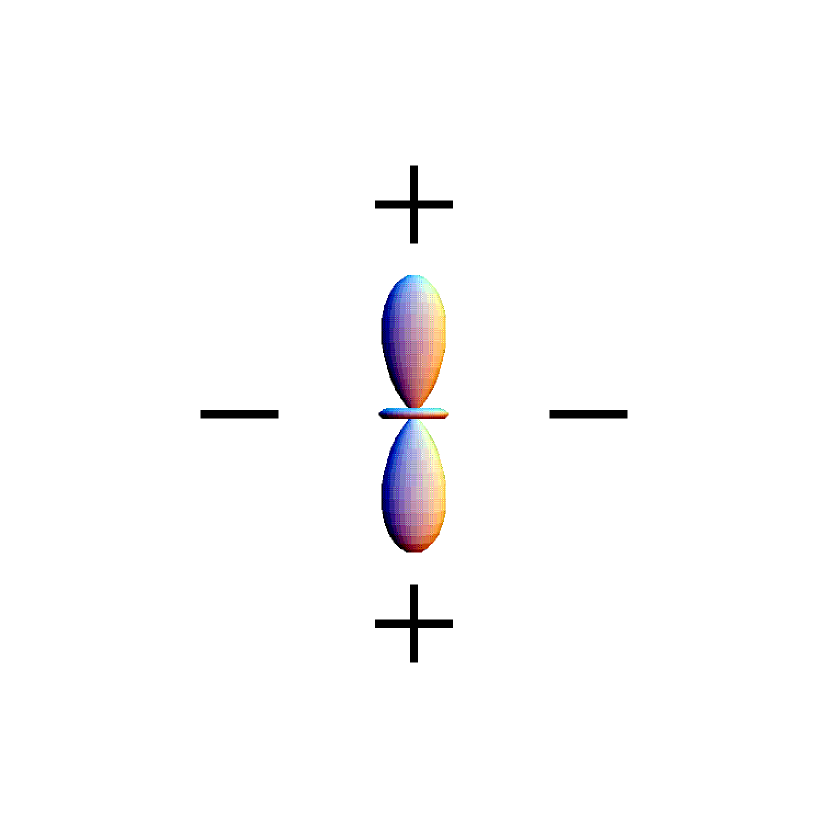
Figure 2: By symmetry, a uniform (monopole) radiation field could not produce any polarization. Left: A dipole radiation field. The direction of the out-going radiation is out of the paper. The plus and minus signs indicate the intensity of the radiation. The light coming from both top and bottom will be polarized perpendicularly to the scattering plane, i.e. along the horizontal direction. The light from the sides will be polarized vertically. Since the sum of the incident light from vertical directions is equal to the sum of the incident light from horizontal directions, the net polarization is zero. Right: A quadrupole radiation field. The direction of the out-going radiation is also out of the paper. The intensity from both the top and the bottom is higher than that from the sides. Therefore the outgoing light has a net polarization in the horizontal direction.

Long before recombination, in thermal equilibrium, both polarization states of photons are equally populated; therefore the incident intensity field should not possess any polarization. In particular, $V=0$. Since Thomson scattering can not generate circular polarization, as discussed in previous section, only $Q$ and $U$ polarization is expected to be present in the CMB.

In this section we assumed that the incident radiation was unpolarized, which is true before recombination. In this case polarization is generated by a quadrupole moment in the incident radiation intensity. If we do allow polarization for the last few scatters before the photons begin to free-stream, there are two additional ways polarized emission can occur: polarized monopole and a polarized quadrupole. These two latter effects are subdominant to the first and we will not describe them in detail here. However, we do keep the polarization monopole and quadrupole terms when we discuss the solution of the cosmological photon Boltzmann equation in section 3.2.

Gravitational wave perturbations can produce outgoing polarized radiation in additional ways which leads to additional terms coupling to the $a_{00}$ component of the incident field as well as higher order terms. We include in our calculation of tensor perturbations in 3.3.

3 Temperature and Polarization Power Spectra

Having outlined how polarization is generated at the last scattering surface we now turn to the prediction of the statistical properties of the polarized CMB. Since the primordial perturbations are expected to be Gaussian to a high degree of accuracy and since linear theory is a highly accurate approximation to the evolution of these perturbations until last scattering, the small anisotropies of temperature and polarization in the CMB are expected to follow Gaussian statistics. That smallness of the anisotropies is also good evidence for global isotropy and homogeneity of the cosmos. These two aspects, Gaussianity and isotropy lead us to believe that the statistics of the anisotropies are comprehensively summarized in the power spectra of the perturbations. These are therefore the central objects of investigation in all current missions observing CMB temperature and polarization.

In this section we follow closely the work of ZS97 for the calculations of the temperature and polarization power spectra of the CMB. With the use of the spin–weighted spherical harmonics, ZS97 unified the treatments of these spectra. We first introduce the basic quantities necessary for the calculations of the perturbations that leave their signature on the CMB (§ 3.1), then detail the calculations of the spectra due to the scalar perturbations (§ 3.2) and tensor perturbations (§ 3.3).

3.1 Definitions

Suppose we are interested in the temperature and polarization anisotropy of CMB at a point ($\theta,\phi$) on the sky. The unit vector along the line of sight is called $\hat{n}$. The Stokes parameters are measured with respect to the local coordinate system specified by the vectors $(\hat{{\rm e}}_{\theta},\hat{{\rm e}}_{\phi})$ on the tangent plane at the point of interest. From Eqn (12) we see that, under a rotation through an angle $\psi$ about $\hat{n}$, a particular combination of Stokes $Q(\hat{n})$ and $U(\hat{n})$ transforms as

$$(Q\pm iU)^{\prime}(\hat{n})={\rm e}^{\mp 2i\psi}(Q\pm iU)(\hat{n}),$$ (44)

i.e., like spin–$\pm 2$ quantities. We therefore can expand them by the spin–2 spherical harmonics:

$$(Q+iU)(\hat{n}) = \sum_{l,m}\,a_{2,lm}\,{}_{2}Y_{lm}(\hat{n}),$$

$$(Q-iU)(\hat{n}) = \sum_{l,m}\,a_{-2,lm}\,{}_{-2}Y_{lm}(\hat{n}).$$ (45)

On the other hand, the temperature anisotropy is expanded by the usual spherical harmonics

$$T(\hat{n}) = \sum_{l,m}\,a_{T,lm}\,Y_{lm}(\hat{n}),$$ (46)

since it is invariant under rotation (spin–0).

With the help of the spin raising and lowering operators, together with Eqn (37), we obtain two spin–$0$ quantities:

$$\flat^{2}\,(Q+iU)(\hat{n}) = \sum_{l,m}\,a_{2,lm}\,\flat\flat\,_{2}Y_{lm}(\hat{n})$$

$$= \sum_{l,m}\,a_{2,lm}\,\flat\left(-\sqrt{(l+2)(l-1)}\,_{1}Y_{lm}\right)$$

$$= \sum_{l,m}\,\left[{(l+2)!\over(l-2)!}\right]^{1/2}a_{2,lm}\,Y_{lm}(\hat{n}),$$

$$\sharp^{2}\,(Q-iU)(\hat{n}) = \sum_{l,m}\,\left[{(l+2)!\over(l-2)!}\right]^{1/2}a_{-2,lm}\,Y_{lm}(\hat{n}).$$ (47)

From these the expansion coefficients can be found by using the orthogonality of spin–$0$ & $2$ spherical harmonics:

$$a_{T,lm} = \int\,d\Omega\,Y_{lm}^{*}(\hat{n})\,T(\hat{n}),$$

$$a_{2,lm} = \int\,d\Omega\,_{2}Y_{lm}^{*}(\hat{n})\,(Q+iU)(\hat{n}),$$

$$= \left[{(l-2)!\over(l+2)!}\right]^{1/2}\int\,d\Omega\,Y_{lm}^{*}(\hat{n})\,\flat^{2}\,(Q+iU)(\hat{n}),$$

$$a_{-2,lm} = \int\,d\Omega\,_{-2}Y_{lm}^{*}(\hat{n})\,(Q-iU)(\hat{n}),$$ (48)

$$= \left[{(l-2)!\over(l+2)!}\right]^{1/2}\int\,d\Omega\,Y_{lm}^{*}(\hat{n})\,\sharp^{2}\,(Q-iU)(\hat{n}).$$

In Appendix A we discuss the parity of $Q$ and $U$ under spatial inversion, the operation that takes $\hat{n}$ into $-\hat{n}$. We find that $Q$ is parity even, $U$ is parity odd. In the following we group together quantities of the same parity, and work with two spin–0 quantities $\widetilde{E}(\hat{n})$ and $\widetilde{B}(\hat{n})$ constructed from $\flat^{2}\,(Q+iU)(\hat{n})$ and $\sharp^{2}\,(Q-iU)(\hat{n})$ (ZS97):

$$\widetilde{E}(\hat{n}) \equiv {-1\over 2}\left(\flat^{2}\,(Q+iU)(\hat{n})+\sharp^{2}\,(Q-iU)(\hat{n})\right)$$ (49)

$$= \sum_{l,m}\left[{(l+2)!\over(l-2)!}\right]^{1/2}\,a_{E,lm}\,Y_{lm}(\hat{n})$$

$$\equiv \sum_{l,m}\,a_{\widetilde{E},lm}\,Y_{lm}(\hat{n}),$$

$$\widetilde{B}(\hat{n}) \equiv {-1\over 2i}\left(\flat^{2}\,(Q+iU)(\hat{n})-\sharp^{2}\,(Q-iU)(\hat{n})\right)$$ (50)

$$= \sum_{l,m}\left[{(l+2)!\over(l-2)!}\right]^{1/2}\,a_{B,lm}\,Y_{lm}(\hat{n})$$

$$\equiv \sum_{l,m}\,a_{\widetilde{B},lm}\,Y_{lm}(\hat{n}),$$

where we have introduced coefficients which are linear combinations of $a_{2,lm}$ and $a_{-2,lm}$:

$$a_{E,lm} \equiv -(a_{2,lm}+a_{-2,lm})/2,$$

$$a_{B,lm} \equiv -(a_{2,lm}-a_{-2,lm})/2i,$$

$$a_{(\widetilde{E},\widetilde{B}),lm} = \left[{(l+2)!\over(l-2)!}\right]^{1/2}a_{(E,B),lm}.$$ (51)

The main advantage of working with $\widetilde{E}$ and $\widetilde{B}$ compared to $Q$ and $U$ is that they are scalar, spin-$0$ quantities. In this way the calculation of polarization spectra proceeds analogously to that of the temperature spectrum. While the same is true for the quantities defined in Eqn (3.1), other advantages of $\widetilde{E}$ and $\widetilde{B}$ are that they are real, and, more importantly, that they have distinct parities (see Appendix A). Under parity transformation the $\widetilde{E}$ pattern remains the same, while that of $\widetilde{B}$ changes sign. It is this property that reduces the number of power spectra (see below) that we need to calculate: cross–correlations between $\widetilde{B}$ and $T$ or $\widetilde{E}$ vanish (see § A).

Finally, let us define the power spectra necessary to describe the statistics of CMB temperature and polarization maps:

$$C_{Xl} = {1\over 2l+1}\sum_{m}\langle a_{X,lm}^{*}\,a_{X,lm}\rangle,$$

$$C_{Cl} = {1\over 2l+1}\sum_{m}\langle a_{T,lm}^{*}\,a_{E,lm}\rangle,$$ (52)

where $X\,=\,T,\,E,\,B$, and $\langle...\rangle$ denotes ensemble average. From Eqn (48) we see that

$$\langle a_{T,l^{\prime}m^{\prime}}^{*}\,a_{T,lm}\rangle=\int\int d\Omega^{\prime}d\Omega\,\langle T^{*}(\hat{n}^{\prime})T(\hat{n})\rangle\,Y_{l^{\prime}m^{\prime}}(\hat{n}^{\prime})Y_{lm}(\hat{n}).$$

If correlation in temperature at different sky positions $\hat{n}^{\prime}$ and $\hat{n}$ can be expressed as $\langle T^{*}(\hat{n}^{\prime})T(\hat{n})\rangle=C_{TT}(\hat{n}^{\prime}\cdot\hat{n})$, i.e. only a function of the angle between the two position vectors, we can expand the correlation function in terms of the Legendre polynomial:

$$C_{TT}(\hat{n}^{\prime}\cdot\hat{n})=\sum_{q}\frac{2q+1}{4\pi}C_{Tq}P_{q}(\hat{n}^{\prime}\cdot\hat{n}).$$

With the help of the addition theorem of spherical harmonics

$$P_{q}(\hat{n}^{\prime}\cdot\hat{n})=\frac{4\pi}{2q+1}\sum_{k}Y_{qk}^{*}(\hat{n}^{\prime})Y_{qk}(\hat{n}),$$

we obtain

$$\langle a_{T,l^{\prime}m^{\prime}}^{*}\,a_{T,lm}\rangle = \sum_{q,k}C_{Tq}\int d\Omega^{\prime}\,Y_{qk}^{*}(\hat{n}^{\prime})Y_{l^{\prime}m^{\prime}}(\hat{n}^{\prime})\int d\Omega\,Y_{qk}(\hat{n})Y_{lm}(\hat{n})$$ (53)

$$= \sum_{q,k}C_{Tq}\,\delta_{ql^{\prime}}\delta_{km^{\prime}}\delta_{ql}\delta_{km}$$

$$= C_{Tl}\,\delta_{ll^{\prime}}\delta_{mm^{\prime}}.$$

Similar calculations lead to other correlations between $T$, $E$, and $B$ modes; we therefore conclude

$$\langle a_{X,l^{\prime}m^{\prime}}^{*}\,a_{X,lm}\rangle = C_{Xl}\,\delta_{l^{\prime}l}\,\delta_{m^{\prime}m},$$

$$\langle a_{T,l^{\prime}m^{\prime}}^{*}\,a_{E,lm}\rangle = C_{Cl}\,\delta_{l^{\prime}l}\,\delta_{m^{\prime}m},$$

$$\langle a_{B,l^{\prime}m^{\prime}}^{*}\,a_{T,lm}\rangle = \langle a_{B,l^{\prime}m^{\prime}}^{*}\,a_{E,lm}\rangle=\ 0.$$ (54)

3.2 Scalar Perturbations

Scalar perturbations (e.g. perturbations of the gravitational potential, see Efstathiou 1990, Ma & Bertschinger 1995, and Dodelson 2003 for detailed treatments and Bertschinger 2000 for a useful summary of structure formation) can be expanded into plane waves, each characterized by a wave vector ${\bf k}$. We can decompose the temperature anisotropy seen by an observer at conformal time $\tau$ into individual contributions from different $\mathbf{k}$-modes of the scalar perturbation. There are only two relevant directions, $\hat{k}$ and the line of sight $\hat{n}$. Without loss of generality we can always choose coordinates such that $\hat{z}\parallel{\bf k}$. We denote this temperature anisotropy by $\Delta_{T}^{s}(\tau,k,\mu)$, which by the above argument only depends on the angle between the photon direction $\hat{n}$ and $\hat{k}$, $\mu\equiv\hat{n}\cdot\hat{k}$, the amplitude of the mode, $k\equiv|{\bf k}|$, and the conformal time $\tau$. The use of “$\Delta$” means the anisotropy is due to this single mode; and the superscript “s” denotes the scalar perturbation.

Unlike the case of temperature anisotropy, for the polarization calculations, we need to specify a local coordinate system for every point on the sky. A “natural” choice is the local unit vectors $\hat{e}_{\theta}$ and $\hat{e}_{\phi}$ of the usual spherical coordinates, together with $\hat{n}$ as the third unit vector, as mentioned in § 3.1. This is a good choice because of two symmetries in the problem: in addition to the azimuthal symmetry, there is also reflection symmetries, that is, space inverse with respect to the plane containing ${\bf k}$ and $\hat{n}$. Under space inverse, $Q$ remains unchanged while $U$ changes sign (see § A). Therefore, under this choice of coordinates, the polarization can only be in either $\hat{e}_{\theta}$ or $\hat{e}_{\phi}$ direction, that is, purely $Q$ with $U=0$. Since $V$ is also zero, the polarization tensor is diagonal in this frame (c.f. Eqn 18).

In short, simple symmetry considerations suggest that only the $Q$ component will be present (which we denote as $\Delta_{Q}^{s}$), and its amplitude depends only on $\mu$, $k$ and $\tau$. We denote the polarization due to this single mode by $\Delta_{P}^{s}(\tau,k,\mu)\equiv\Delta_{Q}^{s}+i\Delta_{U}^{s}$. Specifically, $\Delta_{P}^{s}=\Delta_{Q}^{s}$ in this frame.

The evolution of the anisotropies is described by the Boltzmann equation. In the synchronous gauge, we have (e.g., Ma & Bertschinger 1995)

$$\dot{\Delta}_{T}^{s}+ik\mu\Delta_{T}^{s} = -{1\over 6}\dot{h}-{1\over 3}(\dot{h}+6\dot{\eta})P_{2}(\mu)+\dot{\kappa}\left[-\Delta_{T}^{s}+\Delta_{T0}^{s}+\hat{n}\cdot{\bf v_{b}}-{1\over 2}P_{2}(\mu)\Pi\right],$$

$$\dot{\Delta}_{P}^{s}+ik\mu\Delta_{P}^{s} = \dot{\kappa}\left[-\Delta_{P}^{s}+{3\over 4}(1-\mu^{2})\Pi\right],$$

$$\Pi(\tau,k) = \Delta_{T2}^{s}+\Delta_{P0}^{s}+\Delta_{P2}^{s},$$ (55)

where $h$ and $h+6\eta$ are the trace and traceless scalar parts of the metric perturbation, ${\bf v_{b}}$ is the baryon velocity, and the $\Delta^{s}_{(T,P)j}$ ($j=0,2$) are from the Legendre expansion

$$\Delta(k,\mu)=\sum_{l}(-i)^{l}(2l+1)\Delta_{l}(k)P_{l}(\mu).$$

Using this expansion convention, $\hat{n}\cdot{\bf v_{b}}=-iv_{b}\mu$. The differential optical depth is defined through

$$\dot{\kappa}=a(\tau)\,n_{e}\,x_{e}\,\sigma_{T},\ \ \ \ \ \ \kappa(\tau)=\int_{\tau}^{\tau_{0}}\dot{\kappa}(\tau^{\prime})\,d\tau^{\prime},$$ (56)

where $a(\tau)$ is the cosmic expansion factor, $n_{e}$ is the electron density and $x_{e}$ is the ionization fraction. Note the time derivatives are all with respect to $\tau$.

We caution that $\Delta_{T}^{s}$ defined here is the perturbation of photon brightness temperature, which is $1/4$ of the perturbation in intensity; the latter is adopted by Bond & Efstathiou (1984) with the same notation. The equation (1) in Bond & Efstathiou (1984) is therefore 4 times Eqn (55). Also notice $h_{33}$ in Bond & Efstathiou (1984) is $h+4\eta$ used here.

Note also that the three contributions to $\Pi$, the term which sources polarized photon brightness in Eqn (55), correspond to the contributions discussed in section 2.3.2.

In Appendix B we show how to write down an integral solution to the Boltzmann equation (Seljak & Zaldarriaga, 1996). This method of solving the Boltzmann equation is called the line-of-sight technique, as a way of distinguishing it from traditional techniques such as the moment expansion. The result is

$$\Delta_{T}^{s}(\tau_{0},k,\mu) = \int_{0}^{\tau_{0}}d\tau\,{\rm e}^{-ix\mu}S_{T}^{s}(\tau,k),$$

$$S_{T}^{s}(\tau,k) = {\rm e}^{-\kappa}(\dot{\eta}+\ddot{\alpha})+g(\tau)\left(\Delta_{T0}^{s}+2\dot{\alpha}+{\dot{v_{b}}\over k}+{\Pi\over 4}+{3\ddot{\Pi}\over 4k^{2}}\right)$$

$$+\dot{g}(\tau)\left(\alpha+{v_{b}\over k}+{3\dot{\Pi}\over 2k^{2}}\right)+{3\Pi\ddot{g}(\tau)\over 4k^{2}},$$

$$g(\tau) = \dot{\kappa}\,{\rm e}^{-\kappa},$$

$$\Delta_{P}^{s}(\tau_{0},k,\mu) = {3\over 4}(1-\mu^{2})\int_{0}^{\tau_{0}}d\tau\,{\rm e}^{-ix\mu}\,g(\tau)\,\Pi(\tau,k),$$ (57)

where the auxiliary variable $x=k(\tau_{0}-\tau)$, and $\alpha=(\dot{h}+6\dot{\eta})/2k^{2}$. In particular, the visibility function $g(\tau)$ encodes the ionization/recombination history of the Universe and is strongly peaked at the epoch of recombination. Also notice how simple the $\mu$ dependences are in these solutions.

So far all the calculations are done for one ${\bf k}$ mode; to obtain the total contribution from all modes we need to sum over their contributions. Consider the temperature anisotropy first. At the direction $\hat{n}$ the contribution from scalar perturbations is

$$T^{s}(\hat{n})=\int\,d^{3}{\bf k}\,\xi({\bf k})\,\Delta_{T}^{s}(\tau_{0},k,\mu),$$ (58)

where $\xi({\bf k})$ is a random variable describing the stochastic property of the initial density field; it satisfies

$$\langle\xi^{*}({\bf k}_{1})\,\xi({\bf k}_{2})\rangle=P^{s}(k)\,\delta({\bf k}_{1}-{\bf k}_{2}),$$ (59)

where $P^{s}(k)$ is the primordial power spectrum for scalar perturbations. From this we can calculate the power spectrum $C_{Tl}$ (ZS97):

$$C_{Tl} = {1\over 2l+1}\sum_{m}\langle a_{T,lm}^{*}\,a_{T,lm}\rangle$$ (60)

$$= {1\over 2l+1}\sum_{m}\langle\left(\int\,d\Omega^{\prime}\,Y_{lm}^{*}(\hat{n}^{\prime})\,T^{s}(\hat{n}^{\prime})\right)^{*}\left(\int\,d\Omega\,Y_{lm}^{*}(\hat{n})\,T^{s}(\hat{n})\right)\rangle$$

$$= {1\over 2l+1}\sum_{m}\int\,d\Omega^{\prime}\,d\Omega\,d^{3}{\bf k}^{\prime}\,d^{3}{\bf k}\,Y_{lm}(\hat{n}^{\prime})\,Y_{lm}^{*}(\hat{n})\,$$

$$\mbox{\ \ \ \ \ \ \ \ \ \ \ \ \ \ \ }\times\Delta^{s*}_{T}(\tau_{0},k^{\prime},\mu^{\prime})\,\Delta^{s}_{T}(\tau_{0},k,\mu)\,\langle\xi^{*}({\bf k}^{\prime})\,\xi({\bf k})\rangle$$

$$= {1\over 2l+1}\sum_{m}\int d^{3}{\bf k}\,P^{s}(k)\int\,d\Omega^{\prime}\,d\Omega\,Y_{lm}(\hat{n}^{\prime})\,Y_{lm}^{*}(\hat{n})$$

$$\mbox{\ \ \ \ \ \ \ \ \ \ \ \ \ \ \ }\times\Delta^{s*}_{T}(\tau_{0},k,\hat{n}^{\prime}\cdot\hat{k})\,\Delta^{s}_{T}(\tau_{0},k,\hat{n}\cdot\hat{k})$$

$$= {1\over 2l+1}\int d^{3}{\bf k}\,P^{s}(k)\sum_{m}\left|\int\,d\Omega\,Y_{lm}^{*}(\hat{n})\Delta^{s}_{T}(\tau_{0},k,\mu)\right|^{2}$$

$$= {1\over 2l+1}\int d^{3}{\bf k}\,P^{s}(k)\sum_{m}\left|\int_{0}^{\tau_{0}}d\tau\,S_{T}^{s}(\tau,k)\,\int d\Omega\,Y_{lm}^{*}(\hat{n})\,{\rm e}^{-ix\mu}\,\right|^{2}$$

$$= (4\pi)^{2}\int k^{2}\,dk\,P^{s}(k)\left[\int_{0}^{\tau_{0}}d\tau\,S_{T}^{s}(\tau,k)\,j_{l}(x)\right]^{2}$$

$$= (4\pi)^{2}\int k^{2}\,dk\,P^{s}(k)[\Delta^{s}_{Tl}(k)]^{2},$$

where

$$\Delta^{s}_{Tl}(k)\equiv\int_{0}^{\tau_{0}}d\tau\,S_{T}^{s}(\tau,k)\,j_{l}(x),$$ (61)

and $j_{l}(x)$ is the spherical Bessel function of order $l$. Because of the configuration that $\hat{z}\parallel{\bf k}$, the identity $\int d\Omega\,Y_{lm}^{*}(\hat{n})\,{\rm e}^{-ix\mu}=[4\pi(2l+1)]^{1/2}\,(-i)^{l}\,j_{l}(x)\,\delta_{m0}$ has been used.

Next let us consider the case for polarization. Because under a rotation of the plane perpendicular to $\hat{n}$, the Stokes $Q$ and $U$ change into each other, we need to refer all calculations to a fixed coordinate. In other words, the contributions to polarization anisotropy from all scalar modes are

$$(Q\pm iU)^{s}(\hat{n})=\int\,d^{3}{\bf k}\,\xi({\bf k})\,{\rm exp}(\mp 2i\phi_{\hat{n},\hat{k}})\,\Delta^{s}_{P}(\tau_{0},k,\mu),$$

where $\phi_{\hat{n},\hat{k}}$ is the angle needed to rotate each $\hat{z}\parallel{\bf k}$ frame to the standard reference frame. This is a main source of complications associated with polarization spectra calculations (ZS97). Instead, in complete analogy to the temperature calculations (Eqn 58), we use (ZS97)

$$\widetilde{E}^{s}(\hat{n})=\int\,d^{3}{\bf k}\,\xi({\bf k})\,\Delta^{s}_{\widetilde{E}}(\tau_{0},k,\mu)$$ (62)

to compute the power spectra, where the spin–$0$ quantity $\Delta^{s}_{\widetilde{E}}$ is defined by Eqn (49):

$$\Delta^{s}_{\widetilde{E}}(\tau_{0},k,\mu) = {-1\over 2}\left(\flat^{2}\Delta^{s}_{P}(\tau_{0},k,\mu)+\sharp^{2}\Delta^{s*}_{P}(\tau_{0},k,\mu)\right)$$ (63)

$$= {-3\over 4}\int_{0}^{\tau_{0}}d\tau\,g(\tau)\,\Pi(\tau,k)\partial_{\mu}^{2}\left[(1-\mu^{2})^{2}\,{\rm e}^{-ix\mu}\right]$$

$$= {3\over 4}\int_{0}^{\tau_{0}}d\tau\,g(\tau)\,\Pi(\tau,k)(1+\partial_{x}^{2})^{2}\left(x^{2}\,{\rm e}^{-ix\mu}\right),$$

where we have used the fact that $\Delta^{s}_{P}(\tau_{0},k,\mu)=\Delta^{s*}_{P}(\tau_{0},k,\mu)$ (recall that $\Delta_{U}^{s}=0$) and applied Eqns (25) & (26) to the integral solution Eqn (57). In obtaining the last expression, we have used the fact that $g(\partial_{b})\,[f(b)\,{\rm exp}(-iab)]=g(\partial_{b})\,[f(i\partial_{a})\,{\rm exp}(-iab)]=f(i\partial_{a})\,[g(\partial_{b})\,\,{\rm exp}(-iab)]$ (where $f(y)$ and $g(y)$ are polynomials of $y$) to simplify the $\mu$ dependence. It is apparent from the definition Eqn (50) that

$$\Delta^{s}_{\widetilde{B}}(\tau_{0},k,\mu)={-1\over 2i}\left(\flat^{2}\Delta^{s}_{P}(\tau_{0},k,\mu)-\sharp^{2}\Delta^{s*}_{P}(\tau_{0},k,\mu)\right)=0,$$

thus

$$\widetilde{B}^{s}(\hat{n})=\int\,d^{3}{\bf k}\,\xi({\bf k})\,\Delta^{s}_{\widetilde{B}}(\tau_{0},k,\mu)=0.$$

Therefore the only polarization related power spectra for scalar perturbations that we need to calculate are $C_{El}$ and $C_{Cl}$.

The calculation of $C_{El}$ is now very similar to that of $C_{Tl}$:

$$C_{El} = {1\over 2l+1}\sum_{m}\langle a_{E,lm}^{*}\,a_{E,lm}\rangle$$

$$= {1\over 2l+1}{(l-2)!\over(l+2)!}\times\sum_{m}\langle\left(\int\,d\Omega^{\prime}\,Y_{lm}^{*}(\hat{n}^{\prime})\,\widetilde{E}(\hat{n}^{\prime})\right)^{*}\left(\int\,d\Omega\,Y_{lm}^{*}(\hat{n})\,\widetilde{E}(\hat{n})\right)\rangle$$

$$= {1\over 2l+1}{(l-2)!\over(l+2)!}\sum_{m}\int\,d\Omega^{\prime}\,d\Omega\,d^{3}{\bf k}^{\prime}\,d^{3}{\bf k}\,Y_{lm}(\hat{n}^{\prime})\,Y_{lm}^{*}(\hat{n})\,$$

$$\mbox{\ \ \ \ \ \ \ \ \ \ \ \ \ \ }\times\Delta^{s*}_{\widetilde{E}}(\tau_{0},k^{\prime},\mu^{\prime})\,\Delta^{s}_{\widetilde{E}}(\tau_{0},k,\mu)\,\langle\xi^{*}({\bf k}^{\prime})\,\xi({\bf k})\rangle$$

$$= {1\over 2l+1}{(l-2)!\over(l+2)!}\sum_{m}\int d^{3}{\bf k}\,P^{s}(k)\int\,d\Omega^{\prime}\,d\Omega\,Y_{lm}(\hat{n}^{\prime})\,Y_{lm}^{*}(\hat{n})\Delta^{s*}_{\widetilde{E}}(\tau_{0},k,\hat{n}^{\prime}\cdot\hat{k})\,\Delta^{s}_{\widetilde{E}}(\tau_{0},k,\hat{n}\cdot\hat{k})$$

$$= {1\over 2l+1}{(l-2)!\over(l+2)!}\int d^{3}{\bf k}\,P^{s}(k)\sum_{m}\left|{3\over 4}\int\,d\Omega Y_{lm}^{*}(\hat{n})\int_{0}^{\tau_{0}}d\tau\,g(\tau)\,\Pi(\tau,k)(1+\partial_{x}^{2})^{2}\left(x^{2}\,{\rm e}^{-ix\mu}\right)\right|^{2}$$

$$= (4\pi)^{2}{(l-2)!\over(l+2)!}\int k^{2}dkP^{s}(k)\left({3\over 4}\int_{0}^{\tau_{0}}d\tau\,g(\tau)\,\Pi(\tau,k)([1+\partial_{x}^{2}]^{2}[x^{2}\,j_{l}(x)])\right)^{2},$$

where we have interchanged the order between angular and temporal integrations, and performed the angular integration to obtain the spherical Bessel function. To proceed, we use the differential equation that defines $j_{l}(x)$

$$j_{l}^{\prime\prime}+2j_{l}^{\prime}/x+\left(1-l(l+1)/x^{2}\right)j_{l}=0,$$

(where the primes denote the derivatives with respect to $x$) to replace the $j_{l}^{\prime\prime}$ and $j_{l}^{\prime}$ terms by $j_{l}$ (ZS97):

$$(1+\partial_{x}^{2})^{2}[x^{2}\,j_{l}(x)] = (1+\partial_{x}^{2})(x^{2}\,j_{l}+\partial_{x}(2xj_{l}+x^{2}j_{l}^{\prime}))$$ (64)

$$= (1+\partial_{x}^{2})(2j_{l}+2xj_{l}^{\prime}+l(l+1)j_{l})$$

$$= (2+l(l+1))j_{l}+2xj_{l}^{\prime}+\partial_{x}((4+l(l+1))j_{l}^{\prime}-4j_{l}^{\prime}-2(x-l(l+1)/x)j_{l})$$

$$= l(l+1)(l(l+1)-2)j_{l}/x^{2}$$

$$= (l-1)l(l+1)(l+2)j_{l}/x^{2}.$$

The power spectrum then becomes (ZS97)

$$C_{El} = (4\pi)^{2}{(l+2)!\over(l-2)!}\int k^{2}\,dk\,P^{s}(k)\left[{3\over 4}\int_{0}^{\tau_{0}}d\tau g(\tau)\,\Pi(\tau,k)\,{j_{l}(x)\over x^{2}}\right]^{2}$$ (65)

$$= (4\pi)^{2}\int k^{2}\,dk\,P^{s}(k)[\Delta^{s}_{El}(k)]^{2},$$

where

$$\Delta^{s}_{El}(k) \equiv \left({(l+2)!\over(l-2)!}\right)^{1/2}\int_{0}^{\tau_{0}}d\tau\,S_{E}^{s}(\tau,k)\,j_{l}(x),$$

$$S_{E}^{s}(\tau,k) \equiv {3\over 4}{g(\tau)\Pi(\tau,k)\over x^{2}},$$ (66)

Following similar procedures we obtain the cross correlation power spectrum

$$C_{Cl}=(4\pi)^{2}\int k^{2}dk\,P^{s}(k)\,\Delta^{s}_{Tl}\,\Delta^{s}_{El}.$$ (67)

3.3 Tensor Perturbations

The calculations of power spectra due to tensor perturbations (gravity waves) are basically the same, if somewhat more complicated. The reason is that, for each Fourier mode of the gravity waves, there are two independent “polarizations”, often denoted by “$+$” and “$\times$”. Let $\xi^{+}$ and $\xi^{\times}$ denote independent random variables that characterize the statistics of the gravity waves, their linear combinations will prove to be useful (ZS97)

$$\xi^{1} = (\xi^{+}-i\xi^{\times})/\sqrt{2},$$

$$\xi^{2} = (\xi^{+}+i\xi^{\times})/\sqrt{2},$$ (68)

which satisfy

$$\langle\xi^{1*}({\bf k})\,\xi^{1}({\bf k}^{\prime})\rangle = \langle\xi^{2*}({\bf k})\,\xi^{2}({\bf k}^{\prime})\rangle=P^{t}(k)\,\delta({\bf k}-{\bf k}^{\prime})/2,$$

$$\langle\xi^{1*}({\bf k})\,\xi^{2}({\bf k}^{\prime})\rangle = 0,$$ (69)

where $P^{t}(k)$ is the primordial power spectrum for gravity waves.

For each Fourier mode ${\bf k}$, we choose $\hat{z}\parallel{\bf k}$; in this frame, the temperature and polarization anisotropies due to the tensor perturbation are denoted as $\Delta_{T}^{t}(\tau,{\bf k},\hat{n})$ and $\Delta_{P}^{t}(\tau,{\bf k},\hat{n})\equiv\Delta_{Q}^{t}+i\Delta_{U}^{t}$, where the $\Delta$ reminds us the contribution is from one ${\bf k}$ mode, and the superscript “t” means “tensor”. Note also, because there is no azimuthal symmetry present now, the anisotropies depend on azimuthal angle $\phi$ as well as $\mu\equiv\hat{k}\cdot\hat{n})$. Their explicit form are (Polnarev, 1985; Kosowsky, 1996)

$$\Delta_{T}^{t}(\tau,{\bf k},\hat{n}) = [(1-\mu^{2})\,{\rm e}^{2i\phi}\,\xi^{1}({\bf k})+(1-\mu^{2})\,{\rm e}^{-2i\phi}\,\xi^{2}({\bf k})]\,\widetilde{\Delta}^{t}_{T}(\tau,k,\mu),$$

$$\Delta_{P}^{t}(\tau,{\bf k},\hat{n}) = [(1-\mu)^{2}\,{\rm e}^{2i\phi}\,\xi^{1}({\bf k})+(1+\mu)^{2}\,{\rm e}^{-2i\phi}\,\xi^{2}({\bf k})]\,\widetilde{\Delta}^{t}_{P}(\tau,k,\mu),$$

$$\Delta_{P}^{t*}(\tau,{\bf k},\hat{n}) = [(1+\mu)^{2}\,{\rm e}^{2i\phi}\,\xi^{1}({\bf k})+(1-\mu)^{2}\,{\rm e}^{-2i\phi}\,\xi^{2}({\bf k})]\,\widetilde{\Delta}^{t}_{P}(\tau,k,\mu),$$ (70)

where the new variables $\widetilde{\Delta}^{t}_{T}(\tau,k,\mu)$ and $\widetilde{\Delta}^{t}_{P}(\tau,k,\mu)$ are independent of $\phi$ and satisfy the Boltzmann equation (Polnarev, 1985)

$$\dot{\widetilde{\Delta}^{t}_{T}}+ik\mu\widetilde{\Delta}^{t}_{T} = -\dot{h}-\dot{\kappa}\,(\widetilde{\Delta}^{t}_{T}-\Psi),$$

$$\dot{\widetilde{\Delta}^{t}_{P}}+ik\mu\widetilde{\Delta}^{t}_{P} = -\dot{\kappa}\,(\widetilde{\Delta}^{t}_{P}+\Psi),$$

$$\Psi = {1\over 10}\widetilde{\Delta}^{t}_{T0}+{1\over 7}\widetilde{\Delta}^{t}_{T2}+{3\over 70}\widetilde{\Delta}^{t}_{T4}-{3\over 5}\widetilde{\Delta}^{t}_{P0}+{6\over 7}\widetilde{\Delta}^{t}_{P2}-{3\over 70}\widetilde{\Delta}^{t}_{P4}.$$ (71)

The solutions to these equations can be obtained by the line-of-sight integration (ZS97):

$$\Delta^{t}_{T}(\tau_{0},{\bf k},\hat{n}) = \left((1-\mu^{2})\,{\rm e}^{2i\phi}\,\xi^{1}({\bf k})+(1-\mu^{2})\,{\rm e}^{-2i\phi}\,\xi^{2}({\bf k})\right)\,\int_{0}^{\tau_{0}}\,d\tau\,{\rm e}^{-ix\mu}S^{t}_{T}(\tau,k),$$

$$\Delta_{P}^{t}(\tau_{0},{\bf k},\hat{n}) = \left((1-\mu)^{2}\,{\rm e}^{2i\phi}\,\xi^{1}({\bf k})+(1+\mu)^{2}\,{\rm e}^{-2i\phi}\,\xi^{2}({\bf k})\right)\,\int_{0}^{\tau_{0}}\,d\tau\,{\rm e}^{-ix\mu}S^{t}_{P}(\tau,k),$$

$$\Delta_{P}^{t*}(\tau_{0},{\bf k},\hat{n}) = \left((1+\mu)^{2}\,{\rm e}^{2i\phi}\,\xi^{1}({\bf k})+(1-\mu)^{2}\,{\rm e}^{-2i\phi}\,\xi^{2}({\bf k})\right)\,\int_{0}^{\tau_{0}}\,d\tau\,{\rm e}^{-ix\mu}S^{t}_{P}(\tau,k),$$ (72)

where

$$S^{t}_{T}(\tau,k) = -\dot{h}\,{\rm e}^{-\kappa}+g\,\Psi,$$

$$S^{t}_{P}(\tau,k) = -g\,\Psi.$$ (73)

Next, to obtain spin–0 quantities we need to apply spin raising and lowering operators to the integral solutions (ZS97):

$$\flat^{2}\,\Delta_{P}^{t}(\tau_{0},{\bf k},\hat{n}) = \xi^{1}({\bf k})\int_{0}^{\tau_{0}}\,d\tau\,S^{t}_{P}(\tau,k)\left(-\partial_{\mu}+{2\over 1-\mu^{2}}\right)^{2}\,[(1-\mu^{2})(1-\mu)^{2}\,{\rm e}^{2i\phi}{\rm e}^{-ix\mu}]$$

$$+\xi^{2}({\bf k})\int_{0}^{\tau_{0}}\,d\tau\,S^{t}_{P}(\tau,k)\left(-\partial_{\mu}-{2\over 1-\mu^{2}}\right)^{2}\,[(1-\mu^{2})(1+\mu)^{2}\,{\rm e}^{-2i\phi}{\rm e}^{-ix\mu}]$$

$$= -\xi^{1}({\bf k})(1-\mu^{2})\,{\rm e}^{2i\phi}\,\int_{0}^{\tau_{0}}\,d\tau\,S^{t}_{P}(\tau,k)\left(\hat{\mathcal{E}}(x)-i\hat{\mathcal{B}}(x)\right)\,{\rm e}^{-ix\mu}$$

$$-\xi^{2}({\bf k})(1-\mu^{2})\,{\rm e}^{-2i\phi}\,\int_{0}^{\tau_{0}}\,d\tau\,S^{t}_{P}(\tau,k)\left(\hat{\mathcal{E}}(x)+i\hat{\mathcal{B}}(x)\right)\,{\rm e}^{-ix\mu},$$

$$\sharp^{2}\,\Delta_{P}^{t*}(\tau_{0},{\bf k},\hat{n}) = \xi^{1}({\bf k})\int_{0}^{\tau_{0}}\,d\tau\,S^{t}_{P}(\tau,k)\left(-\partial_{\mu}-{2\over 1-\mu^{2}}\right)^{2}\,[(1-\mu^{2})(1+\mu)^{2}\,{\rm e}^{2i\phi}{\rm e}^{-ix\mu}]$$

$$+\xi^{2}({\bf k})\int_{0}^{\tau_{0}}\,d\tau\,S^{t}_{P}(\tau,k)\left(-\partial_{\mu}+{2\over 1-\mu^{2}}\right)^{2}\,[(1-\mu^{2})(1-\mu)^{2}\,{\rm e}^{-2i\phi}{\rm e}^{-ix\mu}]$$

$$= -\xi^{1}({\bf k})(1-\mu^{2})\,{\rm e}^{2i\phi}\,\int_{0}^{\tau_{0}}\,d\tau\,S^{t}_{P}(\tau,k)\left(\hat{\mathcal{E}}(x)+i\hat{\mathcal{B}}(x)\right)\,{\rm e}^{-ix\mu}$$

$$-\xi^{2}({\bf k})(1-\mu^{2})\,{\rm e}^{-2i\phi}\,\int_{0}^{\tau_{0}}\,d\tau\,S^{t}_{P}(\tau,k)\left(\hat{\mathcal{E}}(x)-i\hat{\mathcal{B}}(x)\right)\,{\rm e}^{-ix\mu},$$

where operators $\hat{\mathcal{E}}(x)\equiv-12+x^{2}\,(1-\partial_{x}^{2})-8x\,\partial_{x}$ and $\hat{\mathcal{B}}(x)\equiv 8x+2x^{2}\,\partial_{x}$ are introduced. In obtaining these expressions, we have worked out the results of the differentiations with respect to $\mu$, and used the trick $f(b)\,{\rm exp}(-iab)=f(i\partial_{a})\,{\rm exp}(-iab)$ again. For example, the $\xi^{1}({\bf k})$ term of $\flat^{2}\,\Delta_{P}^{t}(\tau_{0},{\bf k},\hat{n})$:

$$\left(-\partial_{\mu}+{2\over 1-\mu^{2}}\right)^{2}\,[(1-\mu^{2})(1-\mu)^{2}\,{\rm e}^{-ix\mu}]\! = \!-(1-\mu^{2})\left(-12-8i(1-\mu)x+(1-\mu)^{2}x^{2}\right){\rm e}^{-ix\mu}$$

$$= \!-(1-\mu^{2})\left(-12-8ix-8x\partial_{x}+x^{2}(1-i\partial_{x})^{2}\right){\rm e}^{-ix\mu}$$

$$= \!-\left(\hat{\mathcal{E}}(x)-i\hat{\mathcal{B}}(x)\right)\,(1-\mu^{2}){\rm e}^{-ix\mu}.$$

Notice how these operators simplify the $\mu$ dependence of the expressions. From these we construct $\Delta_{\widetilde{E}}^{t}(\tau_{0},{\bf k},\hat{n})$ and $\Delta_{\widetilde{B}}^{t}(\tau_{0},{\bf k},\hat{n})$:

$$\Delta^{t}_{\widetilde{E}}(\tau_{0},{\bf k},\hat{n}) = {-1\over 2}\left(\flat^{2}\Delta_{P}^{t}(\tau_{0},{\bf k},\hat{n})+\sharp^{2}\Delta_{P}^{t*}(\tau_{0},{\bf k},\hat{n})\right)$$ (74)

$$= (1-\mu^{2})\left({\rm e}^{2i\phi}\,\xi^{1}({\bf k})+{\rm e}^{-2i\phi}\,\xi^{2}({\bf k})\right)\hat{\mathcal{E}}(x)\,\int_{0}^{\tau_{0}}\,d\tau\,{\rm e}^{-ix\mu}S^{t}_{P}(\tau,k),$$

$$\Delta^{t}_{\widetilde{B}}(\tau_{0},{\bf k},\hat{n}) = {-1\over 2i}\left(\flat^{2}\Delta_{P}^{t}(\tau_{0},{\bf k},\hat{n})-\sharp^{2}\Delta_{P}^{t*}(\tau_{0},{\bf k},\hat{n})\right)$$ (75)

$$= -(1-\mu^{2})\left({\rm e}^{2i\phi}\,\xi^{1}({\bf k})-{\rm e}^{-2i\phi}\,\xi^{2}({\bf k})\right)\hat{\mathcal{B}}(x)\,\int_{0}^{\tau_{0}}\,d\tau\,{\rm e}^{-ix\mu}S^{t}_{P}(\tau,k).$$

The total contributions from all ${\bf k}$ modes are then

$$X^{t}(\hat{n})=\int d^{3}{\bf k}\,\Delta_{X}^{t}(\tau_{0},{\bf k},\hat{n}),$$ (76)

where $X=T,\,\widetilde{E},\,\widetilde{B}$. The solution $\Delta^{t}_{T}(\tau_{0},{\bf k},\hat{n})$ is already given in Eqn (72). These are our starting points in calculating the power spectra.

First let us calculate the temperature spectrum:

$$C_{Tl} = {1\over 2l+1}\sum_{m}\langle a_{T,lm}^{*}\,a_{T,lm}\rangle$$

$$= {1\over 2l+1}\sum_{m}\langle\left(\int\,d\Omega^{\prime}\,Y_{lm}^{*}(\hat{n}^{\prime})\,T^{t}(\hat{n}^{\prime})\right)^{*}\left(\int\,d\Omega\,Y_{lm}^{*}(\hat{n})\,T^{t}(\hat{n})\right)\rangle$$

$$= {1\over 2l+1}\sum_{m}\langle\int\,d\Omega^{\prime}\,d\Omega\,d^{3}{\bf k}^{\prime}\,d^{3}{\bf k}\,Y_{lm}(\hat{n}^{\prime})\,Y_{lm}^{*}(\hat{n})\,\Delta^{t*}_{T}(\tau_{0},k^{\prime},\mu^{\prime})\,\Delta^{t}_{T}(\tau_{0},k,\mu)\rangle$$

$$= {1\over 2l+1}\sum_{m}\langle\int\,d\Omega^{\prime}\,d\Omega\,d^{3}{\bf k}^{\prime}\,d^{3}{\bf k}\,Y_{lm}(\hat{n}^{\prime})\,Y_{lm}^{*}(\hat{n})$$

$$\mbox{\ \ \ }\times(1-\mu^{\prime 2})({\rm e}^{-2i\phi^{\prime}}\,\xi^{1*}({\bf k}^{\prime})+{\rm e}^{2i\phi^{\prime}}\,\xi^{2*}({\bf k}^{\prime}))\left(\int_{0}^{\tau_{0}}d\tau\,{\rm e}^{-ix\mu^{\prime}}\,S_{T}^{t}(\tau,k^{\prime})\right)^{*}$$

$$\mbox{\ \ \ }\times\,(1-\mu^{2})({\rm e}^{2i\phi}\,\xi^{1}({\bf k})+{\rm e}^{-2i\phi}\,\xi^{2}({\bf k}))\int_{0}^{\tau_{0}}d\tau\,{\rm e}^{-ix\mu}\,S_{T}^{t}(\tau,k)\rangle$$

$$= {1\over 2l+1}\sum_{m}\int\,d\Omega^{\prime}\,d\Omega\,d^{3}{\bf k}^{\prime}\,d^{3}{\bf k}\,Y_{lm}(\hat{n}^{\prime})\,Y_{lm}^{*}(\hat{n})$$

$$\mbox{\ \ \ }\times(1-\mu^{\prime 2})(1-\mu^{2})\,\left(\int_{0}^{\tau_{0}}d\tau\,{\rm e}^{-ix\mu^{\prime}}\,S_{T}^{t}(\tau,k^{\prime})\right)^{*}\,\int_{0}^{\tau_{0}}d\tau\,{\rm e}^{-ix\mu}\,S_{T}^{t}(\tau,k)$$

$$\mbox{\ \ \ }\times({\rm e}^{2i\phi}{\rm e}^{-2i\phi^{\prime}}+{\rm e}^{-2i\phi}{\rm e}^{2i\phi^{\prime}})\,{1\over 2}\,P^{t}(k)\,\delta({\bf k}-{\bf k}^{\prime})$$

$$= {1\over 2l+1}\sum_{m}\int\,d^{3}{\bf k}\,d\Omega^{\prime}\,d\Omega\,Y_{lm}(\hat{n}^{\prime})\,Y_{lm}^{*}(\hat{n})(1-(\hat{k}\cdot\hat{n})^{2})(1-(\hat{k}\cdot\hat{n}^{\prime})^{2})$$

$$\mbox{\ \ \ }\times\left(\int_{0}^{\tau_{0}}d\tau\,{\rm e}^{-ix\hat{k}\cdot\hat{n}^{\prime}}\,S_{T}^{t}(\tau,k)\right)^{*}\,\left(\int_{0}^{\tau_{0}}d\tau\,{\rm e}^{-ix\hat{k}\cdot\hat{n}}\,S_{T}^{t}(\tau,k)\right)\,{\rm e}^{2i\phi}{\rm e}^{-2i\phi^{\prime}}\,{1\over 2}\,P^{t}(k)$$

$$+{1\over 2l+1}\sum_{m}\int\,d^{3}{\bf k}\,d\Omega^{\prime}\,d\Omega\,Y_{lm}(\hat{n}^{\prime})\,Y_{lm}^{*}(\hat{n})(1-(\hat{k}\cdot\hat{n})^{2})(1-(\hat{k}\cdot\hat{n}^{\prime})^{2})$$

$$\mbox{\ \ \ }\times\left(\int_{0}^{\tau_{0}}d\tau\,{\rm e}^{-ix\hat{k}\cdot\hat{n}^{\prime}}\,S_{T}^{t}(\tau,k)\right)^{*}\,\left(\int_{0}^{\tau_{0}}d\tau\,{\rm e}^{-ix\hat{k}\cdot\hat{n}}\,S_{T}^{t}(\tau,k)\right)\,{\rm e}^{-2i\phi}{\rm e}^{2i\phi^{\prime}}\,{1\over 2}\,P^{t}(k);$$

we will prove the two terms on the right hand side are equal. Let us denote the first term as $t_{I}$, the second term $t_{II}$. The following equations and expressions will be used:

$$\int_{0}^{2\pi}\,d\phi\,{\rm e}^{\pm 2i\phi}\,{\rm e}^{-im\phi}=2\pi\delta_{m\pm 2},$$

the relation between $Y_{lm}$ and associated Legendre polynomials (e.g. Jackson, 1999)

$$Y_{lm}(\mu,\phi)=\left[{2l+1\over 4\pi}{(l-m)!\over(l+m)!}\right]^{1/2}\,P_{lm}(\mu)\,{\rm e}^{im\phi},$$

the explicit form of associated Legendre polynomials

$$P_{lm}(\mu)=(-1)^{m}(1-\mu^{2})^{m/2}{d^{m}\over d\mu^{m}}P_{l}(\mu),$$

and the relation between $P_{lm}(\mu)$ and $P_{l-m}(\mu)$

$$P_{l-m}(\mu)=(-1)^{m}{(l-m)!\over(l+m)!}P_{lm}(\mu).$$

We begin with the term $t_{I}$:

$$t_{I} = {2\pi\over 2l+1}\sum_{m}\int\,k^{2}\,dk\,P^{t}(k)\,\left|\int d\Omega\,Y_{lm}^{*}(\hat{n})\,(1-\mu^{2})\,{\rm e}^{2i\phi}\,\int_{0}^{\tau_{0}}d\tau\,{\rm e}^{-ix\mu}\,S_{T}^{t}(\tau,k)\right|^{2}$$

$$= {2\pi\over 2l+1}\int\,k^{2}\,dk\,P^{t}(k)$$

$$\mbox{\ \ \ }\times\sum_{m}\,\left|\int\,d\phi\,{\rm e}^{i(2-m)\phi}\,\int d\mu\left[{2l+1\over 4\pi}{(l-m)!\over(l+m)!}\right]^{1/2}\,P_{lm}(\mu)\,(1-\mu^{2})\,\int_{0}^{\tau_{0}}d\tau\,{\rm e}^{-ix\mu}\,S_{T}^{t}(\tau,k)\right|^{2}$$

$$= 2\pi^{2}\,{(l-2)!\over(l+2)!}\int\,k^{2}\,dk\,P^{t}(k)\,\left|\int d\mu(1-\mu^{2})\,P_{l2}(\mu)\,\int_{0}^{\tau_{0}}d\tau\,{\rm e}^{-ix\mu}\,S_{T}^{t}(\tau,k)\right|^{2},$$

the second term $t_{II}$ is:

$$t_{II} = {2\pi\over 2l+1}\sum_{m}\int\,k^{2}\,dk\,P^{t}(k)\,\left|\int d\Omega\,Y_{lm}^{*}(\hat{n})\,(1-\mu^{2})\,{\rm e}^{-2i\phi}\,\int_{0}^{\tau_{0}}d\tau\,{\rm e}^{-ix\mu}\,S_{T}^{t}(\tau,k)\right|^{2}$$

$$= {2\pi\over 2l+1}\int\,k^{2}\,dk\,P^{t}(k)$$

$$\mbox{\ \ }\times\sum_{m}\,\left|\int\,d\phi\,{\rm e}^{i(-2-m)\phi}\int d\mu\left[{2l+1\over 4\pi}{(l-m)!\over(l+m)!}\right]^{1/2}P_{lm}(\mu)\,(1-\mu^{2})\!\int_{0}^{\tau_{0}}d\tau\,{\rm e}^{-ix\mu}\,S_{T}^{t}(\tau,k)\right|^{2}$$

$$= 2\pi^{2}\,{(l+2)!\over(l-2)!}\int\,k^{2}\,dk\,P^{t}(k)\,\left|\int d\mu(1-\mu^{2})\,\underbrace{P_{l-2}(\mu)}_{P_{l2}(l-2)!/(l+2)!}\,\int_{0}^{\tau_{0}}d\tau\,{\rm e}^{-ix\mu}\,S_{T}^{t}(\tau,k)\right|^{2}$$

$$= t_{I}=2\pi^{2}\,{(l-2)!\over(l+2)!}\int\,k^{2}\,dk\,P^{t}(k)\,\left|\int_{0}^{\tau_{0}}d\tau\,S_{T}^{t}(\tau,k)\,\int_{-1}^{1}d\mu\,(1-\mu^{2})\,P_{l2}(\mu)\,{\rm e}^{-ix\mu}\right|^{2}.$$

Using the definition of associated Legendre polynomials, the angular integration can be written as

$$\int_{-1}^{1}\,d\mu\,(1-\mu^{2})\,P_{l2}(\mu)\,{\rm e}^{-ix\mu} = \int_{-1}^{1}\,d\mu\,\left({d^{2}\over d\mu^{2}}P_{l}(\mu)\right)(1-\mu^{2})^{2}\,{\rm e}^{-ix\mu}$$

$$= \int_{-1}^{1}\,d\mu\,\left({d^{2}\over d\mu^{2}}P_{l}(\mu)\right)(1+\partial_{x}^{2})^{2}{\rm e}^{-ix\mu}$$

$$= \left.{dP_{l}\over d\mu}(1+\partial_{x}^{2})^{2}{\rm e}^{-ix\mu}\right|^{1}_{-1}-\int_{-1}^{1}\,d\mu\,{dP_{l}\over d\mu}\,(1+\partial_{x}^{2})^{2}(-ix{\rm e}^{-ix\mu})$$

$$= \left.{dP_{l}\over d\mu}{\rm e}^{-ix\mu}(1-\mu^{2})^{2}\right|^{1}_{-1}+\left.P_{l}(\mu)\,(1+\partial_{x}^{2})^{2}(ix{\rm e}^{-ix\mu})\right|^{1}_{-1}$$

$$\mbox{\ \ \ }-\int_{-1}^{1}\,d\mu\,P_{l}(\mu)(1+\partial_{x}^{2})^{2}(x^{2}{\rm e}^{-ix\mu})$$

$$= 0+\left.P_{l}(\mu)\,i(4i\mu-x+\mu^{2}x)\,{\rm e}^{-ix\mu}(1-\mu^{2})^{2}\right|^{1}_{-1}$$

$$\mbox{\ \ \ }-(1+\partial_{x}^{2})^{2}\left(x^{2}\int_{-1}^{1}d\mu\,P_{l}(\mu)\,{\rm e}^{-ix\mu}\right)$$

$$= -2(1+\partial_{x}^{2})^{2}(x^{2}(-i)^{l}\,j_{l}(x)),$$

where we have used

$$\int_{-1}^{1}d\mu\,{\rm e}^{-ix\mu}P_{l}(\mu)=2\,(-i)^{l}\,j_{l}(x).$$

Therefore the temperature power spectrum is (ZS97):

$$C_{Tl} = 2\,t_{I}$$ (77)

$$= 4\pi^{2}\,{(l-2)!\over(l+2)!}\int\,k^{2}\,dk\,P^{t}(k)\,\left|\int_{0}^{\tau_{0}}d\tau\,S_{T}^{t}(\tau,k)\,2(1+\partial_{x}^{2})^{2}(x^{2}(-i)^{l}\,j_{l}(x))\right|^{2}$$

$$= (4\pi)^{2}\,{(l-2)!\over(l+2)!}\int\,k^{2}\,dk\,P^{t}(k)\,\left|\int_{0}^{\tau_{0}}d\tau\,S_{T}^{t}(\tau,k)\,{j_{l}(x)\over x^{2}}\right|^{2}$$

$$= (4\pi)^{2}\int k^{2}\,dk\,P^{t}(k)[\Delta^{t}_{Tl}(k)]^{2},$$

where we have used the expression Eqn (64), the same trick used in calculation of scalar polarization power spectrum, and defined

$$\Delta^{t}_{Tl}(k)\equiv\left[{(l-2)!\over(l+2)!}\right]^{1/2}\int_{0}^{\tau_{0}}d\tau\,S_{T}^{t}(\tau,k)\,{j_{l}(x)\over x^{2}},$$ (78)

where $S_{T}^{t}(\tau,k)$ is given in Eqn (73). Notice the similarities between these expressions and Eqns (60) & (61).

This formulation has a big payoff, because the calculations of remaining spectra are very similar and straightforward. The reason is that the angular dependence of $\Delta^{t}_{\widetilde{E}}(\tau_{0},{\bf k},\hat{n})$ and $\Delta^{t}_{\widetilde{B}}(\tau_{0},{\bf k},\hat{n})$ are the same as that of $\Delta^{t}_{E}(\tau_{0},{\bf k},\hat{n})$. This is clearly shown in Eqns (72), (74) & (75). The difference, namely the operators $\hat{\mathcal{E}}$ and $\hat{\mathcal{B}}$, can be applied after the angular integrations are performed (ZS97). This leads to

$$C_{El} = (4\pi)^{2}\,\int\,k^{2}\,dk\,P^{t}(k)\,\left|\int_{0}^{\tau_{0}}d\tau\,S_{P}^{t}(\tau,k)\,\hat{\mathcal{E}}\,{j_{l}(x)\over x^{2}}\right|^{2}$$ (79)

$$= (4\pi)^{2}\,\int\,k^{2}\,dk\,P^{t}(k)\,\left|\int_{0}^{\tau_{0}}d\tau\,S_{P}^{t}(\tau,k)\,\left[-j_{l}(x)+j_{l}^{\prime\prime}(x)+{2j_{l}(x)\over x^{2}}+{4j_{l}^{\prime}(x)\over x}\right]\right|^{2},$$

$$C_{Bl} = (4\pi)^{2}\,\int\,k^{2}\,dk\,P^{t}(k)\,\left|\int_{0}^{\tau_{0}}d\tau\,S_{P}^{t}(\tau,k)\,\hat{\mathcal{B}}\,{j_{l}(x)\over x^{2}}\right|^{2}$$ (80)

$$= (4\pi)^{2}\,\int\,k^{2}\,dk\,P^{t}(k)\,\left|\int_{0}^{\tau_{0}}d\tau\,S_{P}^{t}(\tau,k)\,\left[2j_{l}^{\prime}(x)+{4j_{l}(x)\over x}\right]\right|^{2}.$$

These equations can be further simplified by integrating by parts the $j_{l}^{\prime}$ and $j_{l}^{\prime\prime}$ terms to increase computational efficiency (ZS97). The source term $S_{P}^{t}(\tau,k)=-g\Psi$ (Eqn 73) makes sure the boundary terms at $\tau=0$ vanish; the boundary terms at $\tau=\tau_{0}$ can be ignored for $l>0$ modes (i.e. excluding the monopole; see the Appendix B). The $j_{l}^{\prime\prime}$ term in the integrand of $C_{El}$ gives $-j_{l}(x)(\ddot{g}\Psi+2\dot{g}\dot{\Psi}+g\ddot{\Psi})/k^{2}$, the $4j_{l}^{\prime}/x$ term gives $-4j_{l}(x)(\dot{g}\Psi/kx+g\dot{\Psi}/kx+g\Psi/x^{2})$; the $2j_{l}^{\prime}$ term in the integrand of $C_{Bl}$ gives $-2j_{l}(x)(\dot{g}\Psi+g\dot{\Psi})/k$. The final expressions are (ZS97)

$$C_{Xl} = (4\pi)^{2}\int k^{2}\,dk\,P^{t}(k)\,[\Delta^{t}_{Xl}(k)]^{2},$$

$$C_{Cl} = (4\pi)^{2}\int k^{2}\,dk\,P^{t}(k)\,\Delta^{t}_{Tl}(k)\,\Delta^{t}_{El}(k),$$ (81)

where $X=T,\,E,\,B$; $\Delta_{Tl}^{t}(k)$ is given in Eqn (78), and

$$\Delta^{t}_{(E,B)l}(k) = \int_{0}^{\tau_{0}}\,d\tau\,S^{t}_{(E,B)}(\tau,k)\,j_{l}(x),$$

$$S^{t}_{E}(\tau,k) = g(\tau)\left(-\Psi+{\ddot{\Psi}\over k^{2}}+{6\Psi\over x^{2}}+{4\dot{\Psi}\over kx}\right)+\dot{g}(\tau)\left({2\dot{\Psi}\over k^{2}}+{4\Psi\over kx}\right)+\ddot{g}(\tau){\Psi\over k^{2}},$$

$$S^{t}_{B}(\tau,k) = g(\tau)\left({4\Psi\over x}+{2\dot{\Psi}\over k}\right)+2\dot{g}(\tau){\Psi\over k}.$$ (82)

4 Summary

We have given a detailed discussion of the physics of polarization in the CMB. Like the temperature anisotropy, polarization is anisotropic over the sky. After a review of the mathematical and physical background (§ 2), we have re-derived the statistical properties of the temperature and polarization anisotropy in terms of the power spectra in the line-of-sight formalism (§ 3, see also Appendices A and B), which are implemented in the code CMBFAST (ZS97). We hope that this uniform treatment will be of value for the beginning theorist learning about polarization and the solution of the linearized cosmological Boltzmann equations. We provide some suggested reading material in the next section.

5 Further Reading

In this review we follow the mathematical formalism developed in Zaldarriaga & Seljak (1997, ZS97) to construct polarization power spectra. Our treatment can be complemented by the article by Hu & White (1997a), who provided vivid visual aids to understanding the physics of polarization. A recent review (Cabella & Kamionkowski, 2004) treated the same subject under the tensor spherical harmonics formalism (Kamionkowski, Kosowsky, & Stebbins, 1997).

The technique presented in ZS97 was for the full-sky in a spatially flat Universe (which is strongly favored by many observations, especially those from the WMAP satellite). Zaldarriaga, Seljak, & Bertschinger (1998) extended the integral solutions and the calculation of polarization field to non–flat Universe models. Hu & White (1997b); Hu et al. (1998) unified the treatments for anisotropies produced by scalar, vector and tensor perturbations. If this guide is to be for beginners, we refer our readers to these treatments for the intermediate level. A quantum mechanically oriented discussion can be found in Kosowsky (1996).

For more details on simulating the CMB polarization maps and their statistical properties, we refer to the discussions in ZS97 (§ V) and Kamionkowski, Kosowsky, & Stebbins (1997). Detailed and general discussions of polarization experiments can be found in, e.g., Seljak (1997); Hu & White (1997b); Zaldarriaga (1998b); Tegmark & de Oliveira-Costa (2001); Kovac et al. (2002); Kogut et al. (2003); Bond et al. (2003); Bunn et al. (2003) and references therein. For more specific discussions on individual polarization experiments (completed or on-going), see e.g. Keating et al. (2001); Hedman et al. (2001); Kovac et al. (2002); Johnson et al. (2003); Montroy et al. (2003); Keating et al. (2003); de Oliveira-Costa et al. (2003); Barkats et al. (2005); Farese et al. (2004); Bowden et al. (2004); Cortiglioni et al. (2004); Leitch et al. (2005); Readhead et al. (2004).

General discussions of the importance of polarization in constraining or breaking degeneracies in cosmological parameters, or helping to discover new physics can be found in, e.g. Zaldarriaga, Spergel, & Seljak (1997); Kosowsky (1999); Eisenstein, Hu & Tegmark (1999); Tegmark et al. (2004) and the references therein. For more specific topics, such as the reionization and polarization, see e.g. Hu (2000); Liu et al. (2001); Haiman & Holder (2003); for weak gravitational lensing and polarization, see e.g. Zaldarriaga & Seljak (1998); Stompor & Efstathiou (1999); Kesden, Cooray, & Kamionkowski (2002); Seljak & Hirata (2004).

For recent general review on CMB and its polarization, see, e.g. Kosowsky (2001); Hu & Dodelson (2002); Zaldarriaga (2003); Challinor (2004). We also recommend the treatments in textbooks by Peacock (1999); Liddle & Lyth (2000); Dodelson (2003) on this topic.

Among the many useful websites that provide up-to-date information or detailed exposures on CMB-related topics, we refer the reader to that of Wayne Hu for CMB tutorials, that of Anthony Banday for a detailed listing of CMB resources, that of Max Tegmark for CMB data analysis, those of Martin White and Ned Wright for cosmology tutorials, and Edmund Bertschinger’s pages for excellent lecture notes on cosmology and structure formation. An online reading list that also provides links to many additional useful websites can be found on Martin White’s page.

Finally, for numerical work we recommend HEALPix, publically available mathematical software for the simulation and analysis of temperature and polarization maps on the sphere (Górski, Hivon & Wandelt, 1999; Górski et al., 2002).

Appendix A Parity of E and B Modes

Here we discuss the properties of Stokes $Q$ and $U$ and $\widetilde{E}$ and $\widetilde{B}$ (namely $E$ and $B$) under parity transformations. The discussion is similar to that of Zaldarriaga (1998a). Let us consider the space inversion $r\rightarrow r$, $\theta\rightarrow\pi-\theta$, $\phi\rightarrow\pi+\phi$. In the language of basis kets used in § 2.1.2, a polarization state is characterized by the expectation value of the Stokes operators. If the the basis kets are chosen as $|\epsilon_{1}\rangle=\hat{e}_{\theta}$, $|\epsilon_{2}\rangle=\hat{e}_{\phi}$, then they are related to their counterparts in the space–inversed frame by $|\epsilon_{1}^{\prime}\rangle=\hat{e}_{\theta}^{\prime}=-|\epsilon_{1}\rangle$ and $|\epsilon_{2}^{\prime}\rangle=\hat{e}_{\phi}^{\prime}=|\epsilon_{2}\rangle$. We therefore see that the expectation values are $Q^{\prime}=Q$ and $U^{\prime}=-U$: $Q$ has even parity, while $U$ has odd parity.

As for the parities of $E$ and $B$, it is useful to notice that $\partial_{\phi^{\prime}}=\partial_{\phi}$, $\partial_{\theta^{\prime}}=-\partial_{\theta}$. Let $\hat{n}$ and $\hat{n}^{\prime}$ refer to the same physical direction in the original and space–inversed frames, respectively. From $(Q+iU)^{\prime}(\hat{n}^{\prime})=(Q-iU)(\hat{n})$ we have, using Eqn (24),

$$\flat^{\prime}(Q+iU)^{\prime}(\hat{n}^{\prime}) = -{1\over\sin^{2}\theta^{\prime}}\left(\partial_{\theta^{\prime}}-{i\over\sin\theta^{\prime}}\partial_{\phi^{\prime}}\right)\sin^{2}\theta^{\prime}\,(Q+iU)^{\prime}(\hat{n}^{\prime})$$

$$= {1\over\sin^{2}\theta}\left(\partial_{\theta}+{i\over\sin\theta}\partial_{\phi}\right)\sin^{2}\theta\,(Q-iU)(\hat{n})$$

$$= -\sharp(Q-iU)(\hat{n}),$$

$$\flat^{\prime 2}(Q+iU)^{\prime}(\hat{n}^{\prime}) = -{1\over\sin\theta^{\prime}}\left(\partial_{\theta^{\prime}}-{i\over\sin\theta^{\prime}}\partial_{\phi^{\prime}}\right)\sin\theta^{\prime}\,\flat^{\prime}(Q+iU)^{\prime}(\hat{n}^{\prime})$$

$$= {1\over\sin\theta}\left(\partial_{\theta}+{i\over\sin\theta}\partial_{\phi}\right)\sin\theta\,\left(-\sharp\,(Q-iU)(\hat{n})\right)$$

$$= \sharp^{2}(Q-iU)(\hat{n}).$$

Similarly, we have $\sharp^{\prime 2}(Q+iU)^{\prime}(\hat{n}^{\prime})=\flat^{2}(Q-iU)(\hat{n})$.

Using these results and the definition of the $\widetilde{E}$ and $\widetilde{B}$ modes,

$$-2\widetilde{E^{\prime}}(\hat{n}^{\prime}) = \flat^{2}(Q+iU)(\hat{n}^{\prime})+\sharp^{2}(Q-iU)(\hat{n}^{\prime}),$$

$$-2i\widetilde{B}(\hat{n}^{\prime}) = \flat^{2}(Q+iU)(\hat{n}^{\prime})-\sharp^{2}(Q-iU)(\hat{n}^{\prime}),$$

we see that

$$-2\widetilde{E^{\prime}}(\hat{n}^{\prime}) = \sharp^{2}(Q-iU)(\hat{n})+\flat^{2}(Q+iU)(\hat{n})=-2\widetilde{E}(\hat{n}),$$

$$-2i\widetilde{B^{\prime}}(\hat{n}^{\prime}) = \sharp^{2}(Q-iU)(\hat{n})-\flat^{2}(Q+iU)(\hat{n})=2i\widetilde{B}(\hat{n}).$$

Therefore $E$ and $\widetilde{E}$ have even parities, while $B$ and $\widetilde{B}$ have odd parities.

Appendix B Line-of-Sight Integral Solution to Boltzmann Equation

In this section we discuss the integral solution to the Boltzmann equation (Seljak & Zaldarriaga, 1996). We first consider the polarization due to scalar perturbations. The Boltzmann equation is

$$\dot{\Delta}_{P}+ik\mu\Delta_{P} = \dot{\kappa}\left[-\Delta_{P}+{3\over 4}(1-\mu^{2})\Pi\right],$$

$$\Pi(\tau,k) = \Delta_{T2}+\Delta_{P0}+\Delta_{P2},$$

where, for brevity, the superscript $s$ is omitted. If we move the term $-\dot{\kappa}\Delta_{P}$ on the right–hand side to the other side of equality, and multiply both sides with ${\rm e}^{ik\mu\tau-\kappa}$, we find the whole expression becomes ${d\over d\tau}(\Delta_{P}\,{\rm e}^{ik\mu\tau-\kappa})$. (Because of the way it is defined, $d\,{\rm e}^{-\kappa}/d\tau=\dot{\kappa}\,{\rm e}^{-\kappa}$; c.f. Eqn 56.) Integrating over the conformal time then gives

$$\int_{0}^{\tau_{0}}\,d\tau\,{d\over d\tau}\,\left(\Delta_{P}\,{\rm e}^{ik\mu\tau-\kappa}\right) = \Delta_{P}\,{\rm e}^{ik\mu\tau_{0}}-\Delta_{P}\,{\rm e}^{-\kappa(\tau=0)}$$

$$= {3\over 4}\,\int_{0}^{\tau_{0}}\,d\tau\,{\rm e}^{ik\mu\tau-\kappa}\,\dot{\kappa}(1-\mu^{2})\Pi,$$

where, by definition, $\kappa(\tau_{0})=0$, ${\rm e}^{-\kappa(\tau_{0})}=1$, and we have used the fact that $\kappa(\tau=0)\rightarrow\infty$ (i.e. the optical depth to the “big bang” is infinite), the $\Delta_{P}\,{\rm e}^{-\kappa(\tau=0)}$ term vanishes; after dividing through the factor ${\rm e}^{ik\mu\tau_{0}}$, we have

$$\Delta_{P}(\tau_{0},k,\mu) = {3\over 4}(1-\mu^{2})\,\int_{0}^{\tau_{0}}\,d\tau\,{\rm e}^{-ix\mu}\,\dot{\kappa}{\rm e}^{-\kappa}\,\Pi,$$

the solution (57), where $x=k(\tau_{0}-\tau)$.

The solution to the temperature anisotropies is obtained analogously. We have

$$\Delta_{T}(\tau_{0},k,\mu) = \int_{0}^{\tau_{0}}\,d\tau\,{\rm e}^{-ix\mu}\,{\rm e}^{-\kappa}\,\left[-{1\over 6}\dot{h}-{1\over 3}(\dot{h}+6\dot{\eta})P_{2}(\mu)+\dot{\kappa}\left(\Delta_{T0}^{s}-i\mu v_{b}-{1\over 2}P_{2}(\mu)\Pi\right)\right].$$

We can further simplify the $\mu$ dependences in the integral by taking the advantage of the ${\rm e}^{-ix\mu}$ term: for an arbitrary function $Y$ of $\tau$ and $\mu$, we have

$$\int_{0}^{\tau_{0}}\!\!d\tau{\rm e}^{-ix\mu}{\rm e}^{-\kappa}Y(\tau,\mu)\! = \!\!\int_{0}^{\tau_{0}}d\tau\,{1\over ik\mu}\,{d{\rm e}^{-ix\mu}\over d\tau}{\rm e}^{-\kappa}\,Y(\tau,\mu)$$

$$= \!\!{1\over ik\mu}\left\{{\rm e}^{-\kappa(\tau_{0})}Y(\tau_{0},\mu)-{\rm e}^{-i\mu k\tau_{0}-\kappa(0)}Y(0,\mu)-\!\int_{0}^{\tau_{0}}\!d\tau{\rm e}^{-ix\mu}{d\over d\tau}\left({\rm e}^{-\kappa}\,Y\right)\right\},$$

the first term on the right-hand side is simply $Y(\tau_{0})$, which can be regarded as a constant contribution to the photon temperature (the “monopole”), and can be ignored since we are only interested in the temperature fluctuations; the second term vanishes because of the damping before the last scattering. Therefore, if $Y(\tau,\mu)$ contains integral powers of $\mu$, we can eliminate its $\mu$ dependences by successive applications of the above identity. To proceed, let us group the terms on the right-hand side of the integral solution by powers of $\mu$. Recall that $\alpha=(\dot{h}+6\dot{\eta})/2k^{2}$, the first two terms in the square brackets reduce to $\dot{\eta}-k^{2}\mu^{2}\alpha$. We therefore have

$$\Delta_{T}(\tau_{0},k,\mu) = \int_{0}^{\tau_{0}}\,d\tau\,{\rm e}^{-ix\mu}\,\left[\left({\rm e}^{-\kappa}\dot{\eta}+g\Delta_{T0}+{1\over 4}g\Pi\right)-iv_{b}g\,\mu-\left(k^{2}\alpha\,{\rm e}^{-\kappa}+{3\over 4}g\Pi\right)\mu^{2}\right],$$

where we have used $g=\dot{\kappa}{\rm e}^{-\kappa}$. Integrating by parts, the term proportional to $\mu$ is replaced by $(\dot{v}_{b}g+v_{b}\dot{g})/k$, while the terms proportional to $\mu^{2}$ give

$$\left(\ddot{\alpha}{\rm e}^{-\kappa}+2\dot{\alpha}g+\alpha\dot{g}\right)+{3\over 4k^{2}}\left(g\ddot{\Pi}+2\dot{g}\dot{\Pi}+\ddot{g}\Pi\right).$$

Grouping these in derivatives with respect to $g$, we recover the source term $S_{T}^{s}(\tau,k)$ in Eqn (57).

References

• Barkats et al. (2005) Barkats, D., et al. 2005, ApJ, 619, L127
• Bennett et al. (2003) Bennett, C. L. et al. 2003, ApJS, 148, 1
• Bertschinger (2000) Bertschinger, E. 2000, astro-ph/0101009
• Bond & Efstathiou (1984) Bond, J. R. & Efstathiou, G. 1984, ApJ, 285, L45
• Bond et al. (2003) Bond, J. R., Contaldi, C., & Pogosyan, D. 2003, Royal Society of London Philosophical Transactions Series A, 361, 2435 (astro-ph/0310735)
• Bowden et al. (2004) Bowden, M., et al. 2004, MNRAS, 349, 321
• Bunn et al. (2003) Bunn, E. F., Zaldarriaga, M., Tegmark, M., & de Oliveira-Costa, A. 2003, Phys. Rev. D, 67, 023501
• Cabella & Kamionkowski (2004) Cabella, P. & Kamionkowski, M. 2004, astro-ph/0403392
• Caderni et al. (1978) Caderni, N., Fabbri, R., Melchiorri, B., Melchiorri, F., & Natale, V. 1978, Phys. Rev. D, 17, 1901
• Challinor (2004) Challinor, A. 2004, astro-ph/0403344
• Chandrasekhar (1960) Chandrasekhar, S. 1960, Radiative Transfer. New York: Dover
• Cortiglioni et al. (2004) Cortiglioni, S., et al. 2004, New Astronomy, 9, 297
• de Oliveira-Costa et al. (2003) de Oliveira-Costa, A., Tegmark, M., Zaldarriaga, M., Barkats, D., Gundersen, J. O., Hedman, M. M., Staggs, S. T., & Winstein, B. 2003, Phys. Rev. D, 67, 023003
• Dodelson (2003) Dodelson, S. 2003, Modern Cosmology. San Diego: Academic Press
• Efstathiou (1990) Efstathiou, G. 1990, in Physics of the Early Universe, eds. J.A. Peacock, A.F. Heavens, A.T. Davies, A. Hilger, p.361
• Eisenstein, Hu & Tegmark (1999) Eisenstein, D. J., Hu, W., & Tegmark, M. 1999, ApJ, 518, 2
• Farese et al. (2004) Farese, P. C., et al. 2004, ApJ, 610, 625
• Goldberg et al. (1966) Goldberg, N. et al. 1966, J. Math. Phys. 8, 2155
• Górski, Hivon & Wandelt (1999) Górski, K. M. , Hivon, E. F., & Wandelt, B. D.  1999, in “Evolution of Large Scale Structure : From Recombination to Garching”, 37
• Górski et al. (2002) Górski, K. M., Banday, A. J., Hivon, E., & Wandelt, B. D. 2002, in ASP Conf. Ser. 281: Astronomical Data Analysis Software and Systems XI, 11, 107
• Haiman & Holder (2003) Haiman, Z. & Holder, G. P. 2003, ApJ, 595, 1
• Hedman et al. (2001) Hedman, M. M., Barkats, D., Gundersen, J. O., Staggs, S. T., & Winstein, B. 2001, ApJ, 548, L111
• Hu (2000) Hu, W. 2000, ApJ, 529, 12
• Hu et al. (1998) Hu, W., Seljak, U., White, M., & Zaldarriaga, M. 1998, Phys. Rev. D, 57, 3290
• Hu & White (1997a) Hu, W. & White, M. 1997a, New Astronomy, 2, 323
• Hu & White (1997b) Hu, W. & White, M. 1997b, Phys. Rev. D, 56, 596
• Hu & Dodelson (2002) Hu, W. & Dodelson, S. 2002, ARA&A, 40, 171
• Jackson (1999) Jackson, J. D. 1999, Classical Electrodynamics. New York: Wiley
• Johnson et al. (2003) Johnson, B. R., et al. 2003, New Astronomy Review, 47, 1067
• Kaiser (1983) Kaiser, N. 1983, MNRAS, 202, 1169
• Kamionkowski, Kosowsky, & Stebbins (1997) Kamionkowski, M., Kosowsky, A., & Stebbins, A. 1997, Phys. Rev. D, 55, 7368
• Keating et al. (2001) Keating, B. G., O’Dell, C. W., de Oliveira-Costa, A., Klawikowski, S., Stebor, N., Piccirillo, L., Tegmark, M., & Timbie, P. T. 2001, ApJ, 560, L1
• Keating et al. (2003) Keating, B. G., Ade, P. A. R., Bock, J. J., Hivon, E., Holzapfel, W. L., Lange, A. E., Nguyen, H., & Yoon, K. 2003, Proc. SPIE, 4843, 284
• Kesden, Cooray, & Kamionkowski (2002) Kesden, M., Cooray, A., & Kamionkowski, M. 2002, Physical Review Letters, 89, 011304
• Kogut et al. (2003) Kogut, A. et al. 2003, ApJS, 148, 161
• Kosowsky (1996) Kosowsky, A. 1996, Ann. Phys. 246, 49
• Kosowsky (1999) Kosowsky, A. 1999, New Astronomy Review, 43, 157
• Kosowsky (2001) Kosowsky, A. 2001, astro-ph/0102402
• Kovac et al. (2002) Kovac, J., Leitch, E. M., Carlstrom, J. E., & Holzapfel, W. L. 2002, Nature, 420, 772
• Leitch et al. (2005) Leitch, E. M., Kovac, J. M., Halverson, N. W., Carlstrom, J. E., Pryke, C., & Smith, M. W. E. 2005, ApJ, 624, 10
• Liddle & Lyth (2000) Liddle, A. & Lyth, D. H. 2000, Cosmological Inflation and Large-Scale Structure. Cambridge, England: Cambridge University Press
• Liu et al. (2001) Liu, G., Sugiyama, N., Benson, A. J., Lacey, C. G., & Nusser, A. 2001, ApJ, 561, 504
• Ma & Bertschinger (1995) Ma, C. & Bertschinger, E. 1995, ApJ, 455, 7
• Montroy et al. (2003) Montroy, T., et al. 2003, New Astronomy Review, 47, 1057
• Negroponte & Silk (1980) Negroponte, J., & Silk, J. 1980, Physical Review Letters, 44, 1433
• Newman & Penrose (1966) Newman, E. & Penrose, R. 1966, J. Math. Phys. 7, 863
• Peacock (1999) Peacock, J. A. 1999, Cosmological Physics. Cambridge, England: Cambridge University Press
• Penrose & Rindler (1986) Penrose, R. & Rindler, W. 1986, Spinors and Space–Time, Vol. 1. Cambridge, England: Cambridge University Press
• Polnarev (1985) Polnarev, A. G. 1985, Soviet Astronomy, 29, 607
• Readhead et al. (2004) Readhead, A. C. S., et al. 2004, Science, 306, 836
• Rees (1968) Rees, M. J. 1968, ApJ, 153, L1
• Rybicki & Lightman (1979) Rybicki, G. B. & Lightman, A. P. 1979, Radiative Processes in Astrophysics. New York: Wiley
• Sakurai (1985) Sakurai, J. J. 1985, Modern Quantum Mechanics. Reading, MA: Addison Wesley
• Seljak (1997) Seljak, U. 1997, ApJ, 482, 6
• Seljak & Hirata (2004) Seljak, U. & Hirata, C. M. 2004, Phys. Rev. D, 69, 043005
• Seljak & Zaldarriaga (1996) Seljak, U. & Zaldarriaga, M. 1996, ApJ, 469, 437
• Stompor & Efstathiou (1999) Stompor, R. & Efstathiou, G. 1999, MNRAS, 302, 735
• Shu (1991) Shu, F. 1991, Physics of Astrophysics, Vol. 1. New York: University Science Books
• Tegmark & de Oliveira-Costa (2001) Tegmark, M. & de Oliveira-Costa, A. 2001, Phys. Rev. D, 64, 3001
• Tegmark et al. (2004) Tegmark, M. et al. 2004, Phys. Rev. D, 69, 103501
• Thorne (1980) Thorne, K. S. 1980, Rev. Mod. Phys. 52, 299
• Varshalovich, Moskalev & Khersonskii (1988) Varshalovich, D. A., Moskalev, A. N., & Khersonskii, V. K., 1988, Quantum Theory of Angular Momentum. Singapore: World Scientific
• Zaldarriaga (1998a) Zaldarriaga, M. 1998a, Ph.D. Thesis (astro-ph/9806122)
• Zaldarriaga (1998b) Zaldarriaga, M. 1998b, ApJ, 503, 1
• Zaldarriaga (2003) Zaldarriaga, M. 2003, astro-ph/0305272
• Zaldarriaga & Seljak (1997) Zaldarriaga, M. & Seljak, U. 1997, Phys. Rev. D, 55, 1830
• Zaldarriaga & Seljak (1998) Zaldarriaga, M. & Seljak, U. 1998, Phys. Rev. D, 58, 023003
• Zaldarriaga, Seljak, & Bertschinger (1998) Zaldarriaga, M., Seljak, U., & Bertschinger, E. 1998, ApJ, 494, 491
• Zaldarriaga, Spergel, & Seljak (1997) Zaldarriaga, M., Spergel, D. N., & Seljak, U. 1997, ApJ, 488, 1