Inconsistency in theories of violent-relaxation

Abstract

We examine an inconsistency in theories of violent-relaxation by Lynden-Bell and Nakamura. The inconsistency arises from the non-transitive nature of these theories: a system that under goes a violent-relaxation, relaxes and then upon an addition of energy, under goes violent-relaxation once again would settle in an equilibrium state that is different from the one that is predicted had the system would go directly from the initial to the final states. We conclude that a proper description of the violent-relaxation process cannot be achieved by equilibrium statistical mechanics approach, but instead a dynamical theory for the coarse-grained phase-space density is needed.

1 Introduction

The main purpose of this paper is to demonstrate that theories predicting a definite statistical equilibrium, dependent only on the energy and the initial volume $\tau(\eta)d\eta$ at phase-space densities in the range $\eta\to\eta+d\eta$, do not predict the same final state when the system undergoes two violent relaxation sessions separated in time, as they do when the two sessions are treated as one. This may be called an inconsistency or at best a lack of transitivity.

Consider an $N$-body gravitating system that starts in some state far from equilibrium, vibrates violently and settles to a dynamically steady state $s_{1}$ that lasts long enough that it may be considered the final product of violent relaxation with energy $E_{1}$. Now suppose that this system suffers a significant tidal disturbance from a passing object that causes violent vibrations and leaves out the system to relax again but now with energy $E_{2}$. There are now two ways of predicting the outcome. Either we take the function $\tau_{0}(\eta)$ giving the volume at each phase-space density from the initial state $s_{0}$, or we use $\tau_{1}(\eta)$ the predicted outcome for that function after the first relaxation process. Of course if we used the fine grained phase-space density both would be the same, but by hypothesis the system lasted so long in state $s_{1}$ that is at “equilibrium”, and only the coarse-grained density can any longer be relevant to the dynamics of the final relaxation. We show that the outcomes predicted with energy $E_{2}$ and volume functions $\tau_{0}(\eta)$ and $\tau_{1}(\eta)$ are certainly different in the Lynden-Bell theory of violent relaxation (Lynden-Bell, 1967), as well as in a more recent theory by Nakamura (Nakamura, 2000).

This paper is organised as follows: in Sec. 2 we give a short overview of some of the difficulties in the theory of violent relaxation, which we feel complement the main subject of this paper. Then in Sec. 3 we demonstrate the non-transitivity of the Lynden-Bell theory of violent relaxation, using the thought experiment that was presented above. In Sec. 4 we give a brief description of Nakamura’s theory which is based on the information-theory approach. We re-derive his theory using a combinatorial approach that enables us to compare it to Lynden-Bell’s theory. Then in Sec. 5 we demonstrate that also Nakamura’s theory is non-transitive, using the thought experiment once again. In Sec. 6 we present our conclusions.

2 An overview of the difficulties in the theory of violent relaxation

In this section we offer a short discussion of other problems connected with the process of violent-relaxation and ‘theories’ that aim to predict its outcome. Let us start from first principles. Most large $N$-body systems governed by long-range forces which are not initially in balance will oscillate with decreasing amplitude before they settle into a state in which the potential of the long range force becomes almost steady. Such violent-relaxation processes are known to occur in gravitational $N$-body systems. Thereafter evolution may continue due to the shorter range interaction in which the graininess of the individual particles is of importance, but there is a large class of systems in which this secondary evolution is on a much longer timescale. Violent relaxation under gravity does not last long. After a few oscillations on the timescale $(G\bar{\rho})^{-1/2}$ it is over. Thus the whole idea that the interaction of the particles with the mean field will lead to some unique detailed statistical equilibrium state, only dependent on the initial conditions via the dynamically conserved quantities, is more of a vain hope and a confession of ignorance than an established fact. Nevertheless, Hénon (1968) gave some evidence in favour of its prediction and for cosmological initial conditions Navarro, Frenk & White (1995, 1996, 1997) show a considerable universality in their results. Binney (2004) gives a lovely toy model which he uses to criticise deductions from $N$-body simulations. Even in the initial discussion (Lynden-Bell, 1967) it was admitted that there were many stable steady states into which a gravitating system could settle and that violent relaxation would be incomplete so that the system would not inevitably attain a state close to the more probable one.

A second worrying aspect of any equilibrium theory is the apparent lack of an analogue to the law of detailed balance. At real thermodynamic equilibrium there are no cyclic processes going around and around, but each individual emission process is exactly balanced by the corresponding absorption process. In radiation theory Einstein introduced his stimulated emission process just to ensure that this would be so. In the process of violent relaxation each element is interacting with the potential of the whole system, and one might expect some to be highly accelerated as Fermi argued to get his cosmic ray acceleration process. Conservation of energy must however lead to some dynamical friction term but this cannot be mass related as that is at odds with our earlier arguments that energy gain is independent of mass.

Finally, not all systems have violent relaxation. In some early experiments with pulsating concentric spherical shells, Hénon (1968) found a few examples of gravitating system with persistent oscillation that defied the general decay. Newton in Principia showed that systems with a force law between particles proportional to separation (rather than inverse square) oscillated forever. Indeed Newton solved that $N$-body problem completely, showing that each particle moved on a central ellipse centred on the barycentre and that all those orbits had the same period. Lynden-Bell & Lynden-Bell (1999a) showed that Newton’s work could be extended to all systems in which the total potential energy was any function $V(r)$ where $r^{2}=\sum_{i}m_{i}(\mathbf{r}_{i}-\bar{\mathbf{r}})^{2}/M=\frac{1}{2}\sum_{i,j}m_{i}m_{j}(\mathbf{r}_{i}-\mathbf{r}_{j})^{2}/M$ and $\bar{\mathbf{r}}$ is the position of the barycentre. Likewise, the $N$-particle Schrodinger equation was exactly solved for such potentials (Lynden-Bell & Lynden-Bell, 1999b); the most interesting example of which is probably $V=GM^{2}/r$. This has a force between any two particles of $Gm_{i}m_{j}(\mathbf{r}_{i}-\mathbf{r}_{j})/r^{3}$ with the final $r^{3}$ not $|\mathbf{r}_{i}-\mathbf{r}_{j}|^{3}$ but the $r$ defined above. A related exception to violent relaxation with a most interesting ever-pulsating detailed “Maxwellian” statistical equilibrium is the system with an inter-particle potential $\frac{1}{2}m_{i}m_{j}(kr_{ij}^{2}+k^{\prime}r^{-2}_{ij})$. In spite of the complication of the individual particle motions due to the inverse cubic repulsion between particles, such systems pulsate in scale forever in exact undamped simple harmonic motion (Lynden-Bell & Lynden-Bell, 2004).

3 Non-transitivity in the Lynden-Bell theory of violent relaxation

The Lynden-Bell theory of violent relaxation (hereafter LB67) aims at predicting the final equilibrium state of a collisionless gravitating system undergoing a violent relaxation. In order to demonstrate its non-transitive nature we shall first recall its main results for the general case where initially the system has more than one phase-space density levels.

3.1 Main results of the LB67 theory

In the LB67 theory we deal with a system which is initially out of equilibrium. Its initial state is specified by its total energy $E$ and the phase-space volumes $V_{1},V_{2},\ldots$ of the initial phase-space density levels $\eta_{1},\eta_{2},\ldots$. Phase-space is then divided into micro-cells of fixed volume $\tilde{\omega}$, which can be either empty or hold a phase-space element of one of the prescribed levels. The state of all these micro-cells defines a micro-state.

Next, we let the system re-distribute its phase-space elements as it approaches an equilibrium. The micro-cells are then grouped into macro-cells, each macro-cell containing $\nu$ micro-cells. A macro-state of the system is defined by the matrix $\{n_{iJ}\}$ which specifies how many phase-space elements of type $J$ ended up in the macro-cell $i$. The coarse-grained phase-space density function (DF) at the macro-cell $i$ is therefore given by

$$f_{i}=\frac{1}{\nu}\sum_{J}\eta_{J}n_{iJ}\ .$$ (1)

Then, in the spirit of ordinary statistical mechanics, one assumes that the system has an equal a priori probability of being in each one of the micro-states. To find the equilibrium state one maximises the function $W\big{(}\{n_{iJ}\}\big{)}$ which counts the number of micro-states that correspond to the macro-state $\{n_{iJ}\}$, hence obtaining the most probable state.

When maximising $W$ one has to consider only those macro-states for which the total energy is $E$ and the overall volume in each of the initial phase-space levels is $V_{1},V_{2},\ldots$. This can be done in the usual way with Lagrange multipliers. After passing to a continuous description of the macro-cells, the resultant DF is

$$f_{LB}(\mathbf{r},\mathbf{v})=f_{LB}[\epsilon(\mathbf{r},\mathbf{v})]\equiv A(\epsilon)\sum_{J}\eta_{J}e^{-\beta\eta_{J}(\epsilon-\mu_{J})}\ ,$$ (2)

with

$$A(\epsilon)\equiv\frac{1}{1+\sum_{J}e^{-\beta\eta_{J}(\epsilon-\mu_{J})}}\ .$$ (3)

Here $\epsilon(\mathbf{r},\mathbf{v})=v^{2}/2+\Phi_{LB}(r)$ is the energy per unit mass of the $(\mathbf{r},\mathbf{v})$ phase-space cell, $\Phi_{LB}(r)$ is the gravitational potential, calculated self-consistently from the Poisson equation

$$\nabla^{2}\Phi(r)=4\pi G\int\!\!d^{3}\mathbf{v}\,f_{LB}(\mathbf{r},\mathbf{v})\ .$$ (4)

The dimensional constants $\beta,\mu_{1},\mu_{2},\ldots$ are the Lagrange multipliers, which are calculated from the energy conservation constraint

$$\int\!\!d^{6}\tau\,f_{LB}(\mathbf{r},\mathbf{v})\left[\frac{v^{2}}{2}+\frac{1}{2}\Phi_{LB}(r)\right]=E\ ,$$ (5)

and the initial conditions constraints

$$\int\!\!d^{6}\tau\,A(\epsilon)e^{-\beta\eta_{J}(\epsilon-\mu_{J})}=V_{J}\ ,\quad J=1,2,\ldots\ ,$$ (6)

where we have used used the notation $d^{6}\tau\equiv d^{3}\mathbf{r}d^{3}\mathbf{v}$.

Equations (2-6) are the main results of the LB67 theory. For our needs, however, two small modifications are needed. Firstly, by introducing the energy density function

$$g(\epsilon_{0})\equiv\int\!\!d^{6}\tau\,\delta[\epsilon(\mathbf{r},\mathbf{v})-\epsilon_{0}]\ ,$$ (7)

the integral in the LHS of Eq. (6) can be written as $\int\!\!g(\epsilon)A(\epsilon)e^{-\beta\eta_{J}(\epsilon-\mu_{J})}\,d\epsilon$. Secondly, we pass to a continuous description of the initial density levels using the phase-space volume distribution function $\tau(\eta)$, which is defined so that $\tau(\eta)d\eta$ is the phase-space volume initially occupied by phase-space densities in the range $\eta\to\eta+d\eta$. Formally, if $f_{I}(\mathbf{r},\mathbf{v})$ is the initial DF then $\tau(\eta)$ is given by

$$\tau(\eta)=\int\!\!d^{6}\tau\,\delta[f_{I}(\mathbf{r},\mathbf{v})-\eta]\ .$$ (8)

By letting each density level $\eta_{J}$ have a small width $\Delta\eta$, the $\sum_{J}$ sums in Eqs. (2, 3) can be changed to integrals by

$$\sum_{J}\to\frac{1}{\Delta\eta}\int\!\!d\eta\ ,$$ (9)

hence Eqs. (2-6) are now

$$f_{LB}(\epsilon) = \frac{1}{\Delta\eta}A(\epsilon)\int\!\!\eta e^{-\beta\eta(\epsilon-\mu_{\eta})}\,d\eta\ ,$$ (10)

$$A(\epsilon) = \frac{1}{1+\frac{1}{\Delta\eta}\int\!\!e^{-\beta\eta(\epsilon-\mu_{\eta})}\,d\eta}\ ,$$ (11)

$$\nabla^{2}\Phi(r) = 4\pi G\int\!\!d^{3}\mathbf{v}\,f_{LB}(\mathbf{r},\mathbf{v})\ ,$$ (12)

$$E = \int\!\!d^{6}\tau\,f_{LB}(\mathbf{r},\mathbf{v})\left[\frac{v^{2}}{2}+\frac{1}{2}\Phi(r)\right]\ ,$$ (13)

$$\tau(\eta)\Delta\eta = \int\!\!g(\epsilon)A(\epsilon)e^{-\beta\eta(\epsilon-\mu_{\eta})}\,d\epsilon\ .$$ (14)

Notice that the amplitude of $\Delta\eta$ is unimportant as it can always be absorbed into the Lagrange multipliers $\mu_{\eta}$.

Finally we recall that in a spatially infinite domain equations (10-14) have no solution since the density can spread indefinitely while conserving its energy and increasing its entropy. A common way to overcome this problem, which shall be adopted here, is to work within an rigid sphere of radius $R$, and to assume that the resulting equilibrium configuration is spherical. Such model, although not realistic, is an easy way to obtain a finite solution.

3.2 The double relaxation experiment

To test the transitivity of the LB67 theory we propose the following four-steps thought experiment which was mentioned in the introduction:

1. We prepare a system with one density-level (the water-bag configuration) and a total energy of $E$. In accordance with the above section, we put the system inside a sphere of radius $R$. We denote the initial state of the system by $s_{0}$.

2. We let the system go trough a violent relaxation process to an equilibrium which is denoted by $s_{1}$.

3. We add an amount of $\Delta E$ energy to the system by, for example, a strong impulse of an external gravitational field. The system then goes once again through a violent relaxation process and settles down in a new equilibrium state, denoted by $s_{2}$.

4. We prepare a new system with the same parameters as $s_{0}$ except for the energy, which is set to $E+\Delta E$. We let it go through a violent relaxation process to an equilibrium which is denoted by $s_{3}$.

Now if the theory is transitive then necessarily $s_{2}=s_{3}$.

To see if this is really the case in the LB67 theory, we begin by calculating the $s_{1}$ and $s_{3}$ states which are relatively simple to calculate, being the outcome a water-bag configuration. This calculation has been fully done in Chavanis & Sommeria (1998), and here we use some of their results.

The $s_{0}$ step was prepared with total mass $M=1,G=1,R=1$ and an initial phase-space density level

$$\eta_{0}=\frac{10^{3}}{\sqrt{512\pi^{4}G^{3}MR^{3}}}\ ,$$ (15)

which according to Chavanis & Sommeria (1998) guarantees that for each energy there would be only one equilibrium state.

From Eq. (2) we find that the DF of $s_{1}$ and $s_{3}$ is the well-known Fermi-Dirac distribution

$$f_{1}(\epsilon) = \frac{\eta_{0}}{1+e^{\beta_{1}\eta_{0}(\epsilon-\mu_{1})}}\ ,$$ (16)

$$f_{3}(\epsilon) = \frac{\eta_{0}}{1+e^{\beta_{3}\eta_{0}(\epsilon-\mu_{3})}}\ ,$$ (17)

with $\beta_{1},\beta_{3},\mu_{1},\mu_{3}$ Lagrange multipliers to be fixed from the energy constraint and the initial conditions. As there is only one density-level, the initial condition constraint can be replaced with the conservation of mass constraint.

In Chavanis & Sommeria (1998) it is shown how the Lagrange multipliers can be found for a given mass and energy, and we therefore do not repeat these steps here but instead give the values of these parameters in Table 1. All numerical calculations were done using the GNU Scientific Library 1.5 (GSL 1.5), which is a free software available from http://www.gnu.org/software/gsl/. The differential equation for $\Phi(r)$ was solved using an embedded Runge-Kutta Prince-Dormand (8,9) method, whereas integration was done using a 51 points Gauss-Kronrod rule. In all calculations a relative error of less than $10^{-3}$ was maintained.

Figure 1 shows the radial density profiles of $s_{1}$ and $s_{3}$. As the $s_{3}$ configuration is more energetic, its mean kinetic energy is higher and as a result the distribution is less concentrated than the $s_{1}$ distribution, and has a lower density core. Figure 2 shows the DFs of $s_{1}$ and $s_{3}$. Notice how both distributions have a substantial degenerate part, as for both configurations the Fermi energies are $\epsilon_{\alpha_{i}}\simeq\Phi_{i}(0)/2$.

Finally, to verify that the $s_{3}$ configuration is indeed more mixed than the $s_{1}$ configuration - and therefore a transition $s_{1}\to s_{3}$ is permitted by the mixing theorem (Tremaine, Hénon & Lynden-Bell, 1986) - we have calculated the $M(V)$ functions of $s_{1}$ and $s_{3}$. The $M(V)$ function is defined in the following way: we first define $M(\eta)$ and $V(\eta)$ as the cumulative mass and phase-space volumes above the phase-space density $\eta$,

$$V(\eta) \equiv \int_{r<R}\!\!d^{6}\tau\,H[f(\mathbf{r},\mathbf{v})-\eta]=\int_{\eta}^{\infty}\!\!\tau(\eta^{\prime})\,d\eta^{\prime}\ ,$$ (18)

$$M(\eta) \equiv \int_{r<R}\!\!d^{6}\tau\,H[f(\mathbf{r},\mathbf{v})-\eta]=\int_{\eta}^{\infty}\!\!\eta^{\prime}\tau(\eta^{\prime})\,d\eta^{\prime}\ ,$$ (19)

with $H(\cdot)$ being the Heaviside step function. As $V(\eta)$ is a monotonically decreasing function, we can invert it and express $\eta$ in terms of the cumulative volume $V$. Plugging this into $M(\eta)$ we get the $M(V)$ function. According to the mixing theorem, the distribution $s_{3}$ is more mixed than the distribution $s_{1}$ if and only if $M_{3}(V)\leq M_{1}(V)$ for every $V$, as is shown in Fig. 3.

Table 1: The numerical parameters that specify the $s_{1}$ and $s_{3}$ states. $E$ is the total energy of the state, $\eta_{0}$ is the initial density level given by Eq. (15), $\beta,\mu$ are the Lagrange multipliers in Eqs. (16, 17), and $\Phi(0)$ is the gravitational potential at $r=0$.

State	$E$	$\eta_{0}\beta$	$\mu$	$\Phi(0)$
$s_{1}$	$-6.157$	$1.2$	$-14.87$	$-33.96$
$s_{2}$	$-1.589$	$1.0$	$-8.322$	$-15.12$

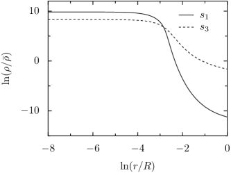
Figure 1: Density profiles of the $s_{1}$ and $s_{3}$ states in the double-relaxation experiment of the LB67 theory. $\bar{\rho}$ is the average density given by $\bar{\rho}=3M/(4\pi R^{3})$. The $s_{3}$ state corresponds to a hotter system with higher energy which makes it less concentrated.

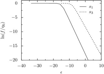
Figure 2: The phase-space densities of $s_{1}$ and $s_{3}$ as functions of the energy per unit mass $\epsilon$. The functional form of these densities is the well-known Fermi-Dirac distribution, given by Eqs. (16, 17) and Table. 1

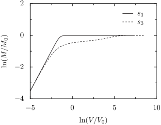
Figure 3: The $M(V)$ functions of $s_{1}$ and $s_{3}$. $M_{0}=1$ is the total mass and $V_{0}=1$ is the initial phase-space volume that is occupied by the density level $\eta_{0}$. We notice that $M_{3}(V)\leq M_{1}(V)$ for every $V$ and therefore $s_{3}$ is more mixed than $s_{1}$ according to the mixing-theorem.

3.3 Analysing the $s_{2}$ configuration

Let us now turn our attention to the $s_{2}$ configuration. Seemingly, we need to calculate the $\tau_{1}(\eta)$ function of the $s_{1}$ configuration, and together with an energy of $E+\Delta E$, solve the equations

$$f_{2}(\epsilon) = \frac{1}{\Delta\eta}A(\epsilon)\int_{0}^{\eta_{0}}\!\!\eta e^{-\beta_{2}\eta(\epsilon-\mu_{\eta})}\,d\eta\ ,$$ (20)

$$A(\epsilon) = \frac{1}{1+\frac{1}{\Delta\eta}\int_{0}^{\eta_{0}}\!\!e^{-\beta_{2}\eta(\epsilon-\mu_{\eta})}\,d\eta}\ ,$$ (21)

$$\tau_{1}(\eta) = \frac{1}{\Delta\eta}\int_{\Phi_{2}(0)}^{\infty}\!\!g_{2}(\epsilon)A(\epsilon)e^{-\beta_{2}\eta(\epsilon-\mu_{\eta})}\,d\epsilon\ .$$ (22)

The function $g_{2}(\epsilon)$ needs to be calculated from Eq. (7) using the gravitational potential $\Phi_{2}(r)$, which has to be recovered from $f_{2}(\epsilon)$ using the Poisson equation (12). Finally, the resultant $f_{2}(\epsilon)$ would be compared to $f_{3}(\epsilon)$ to see if the two configurations are equal.

There is, however, a much simpler way to see if $f_{2}(\epsilon)=f_{3}(\epsilon)$. Let us assume that indeed this is the case, and that consequently also $\Phi_{2}(r)=\Phi_{3}(r)$ and $g_{2}(\epsilon)=g_{3}(\epsilon)$. In such case it is possible to recover the full expression $\frac{1}{\Delta\eta}A(\epsilon)e^{-\beta_{2}\eta_{0}(\epsilon-\mu_{\eta})}$ in terms of the known functions $f_{3}(\epsilon)$ and $g_{3}(\epsilon)$.

We start by replacing $f_{2}(\epsilon)\leftrightarrow f_{3}(\epsilon)$ and $g_{2}(\epsilon)\leftrightarrow g_{3}(\epsilon)$ in Eqs. (20-22). Differentiating Eq. (21) with respect to $\epsilon$ and substituting $f_{3}(\epsilon)$ from Eq. (20), we obtain

$$A^{\prime}_{2}(\epsilon)=\beta_{2}A(\epsilon)f_{3}(\epsilon)\ ,$$ (23)

which yields

$$A(\epsilon)=a_{0}\exp\left(-\beta_{2}\int_{\epsilon}^{\infty}\!\!f_{3}(\epsilon^{\prime})d\epsilon^{\prime}\right)\equiv a_{0}A_{0}(\epsilon)\ .$$ (24)

Here $a_{0}$ is an unknown integration constant. The integral in $A_{0}(\epsilon)$ can be easily done analytically if we recall the definition of $f_{3}(\epsilon)$ which is given in Eq. (17), yielding

$$A_{0}(\epsilon)=\left[1+e^{-\beta_{3}\eta_{0}(\epsilon-\mu_{3})}\right]^{-\frac{\beta_{2}}{\beta_{3}}}\ .$$ (25)

Having found $A(\epsilon)$, we use Eq. (22) to find the Lagrange multipliers $\mu_{\eta}$:

$$e^{-\beta_{2}\eta\mu_{\eta}}=\big{[}\tau_{1}(\eta)\big{]}^{-1}a_{0}\frac{1}{\Delta\eta}\int_{\Phi_{3}(0)}^{\infty}\!\!g_{3}(\epsilon)A_{0}(\epsilon)e^{-\beta_{2}\eta\epsilon}\,d\epsilon\ .$$ (26)

Therefore

$$A(\epsilon)\frac{1}{\Delta\eta}e^{-\beta_{2}\eta(\epsilon-\mu_{\eta})}=\frac{\tau_{1}(\eta)}{B_{0}(\eta)}A_{0}(\epsilon)e^{-\beta_{2}\eta\epsilon}\ ,$$ (27)

with

$$B_{0}(\eta)\equiv\int_{\Phi_{3}(0)}^{\infty}\!\!g_{3}(\epsilon^{\prime})A_{0}(\epsilon^{\prime})e^{-\beta_{2}\eta\epsilon^{\prime}}\,d\epsilon^{\prime}\ .$$ (28)

This finally gives us

$$f_{2}(\epsilon)=A_{0}(\epsilon)\int_{0}^{\eta_{0}}\!\!\frac{\tau_{1}(\eta)}{B_{0}(\eta)}e^{-\beta_{2}\eta\epsilon}\,d\eta\ .$$ (29)

Note that the unknown integration constant $a_{0}$ has been cancelled out. The only remaining unknown is $\beta_{2}$ which can be fixed by requiring that the energy of $s_{2}$ will be equal to $E+\Delta E$. Once this is done, we have an expression for $f_{2}(\epsilon)$ which is equal to $f_{3}(\epsilon)$ if and only if $s_{2}$ is identical to $s_{3}$.

The procedure above is mathematically straightforward, however, numerically it is slightly more complicated as the $\tau_{1}(\eta)$ has a very strong peak near $\eta=\eta_{0}$ due to the degeneracy. It is therefore preferable to perform the calculation using the cumulative version of $\tau_{1}(\eta)$, which was defined in (18). For a spherical, isotropic system in a sphere of radius $R$ with a DF $f(\epsilon)$ and a gravitational potential $\Phi(r)$, it is easy to verify that $V(\eta)$ is given by

$$V(\eta)=\frac{2^{3/2}(4\pi)^{2}}{3}\int_{0}^{r(\eta)}\!\!s^{2}[\epsilon(\eta)-\Phi(s)]^{3/2}\,ds\ ,$$ (30)

with $\epsilon(\eta)$ being the inverse function of $f(\epsilon)$, and $r(\eta)$ is

$$r(\eta)\equiv\left\{\begin{array}[]{lcl}\Phi^{-1}[\epsilon(\eta)]&,&\epsilon(\eta)<-GM/R\\ R&,&\epsilon(\eta)\geq-GM/R\end{array}\right.\ .$$ (31)

Once $V_{1}(\eta)$ is calculated from the formula above [using $f_{1}(\epsilon)$ and $\Phi_{1}(\epsilon)$], we can calculate $f_{2}(\epsilon)$ from Eq. (29) using integration by parts:

$$f_{2}(\epsilon)=A_{0}(\epsilon)\int_{0}^{\eta_{0}}\!\!V_{1}(\eta)\frac{e^{-\beta_{2}\eta\epsilon}}{B_{0}(\eta)}\Big{[}1-\beta_{2}\eta\epsilon-\eta\frac{B^{\prime}_{0}(\eta)}{B_{0}(\eta)}\Big{]}\,d\eta\ .$$ (32)

3.4 Results

To satisfy the energy constraint $E_{2}=E_{3}=-1.589$, we calculated $E_{2}$ for various values of $\beta_{2}$ and chose $\beta_{2}=0.37071$ which gives the correct energy as shown in Fig. 4. We did not find any other solution in the range $0.1<\beta<100$ and therefore we believe that $\beta_{2}=0.37071$ is the only relevant solution.

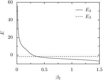
Figure 4: The energy $E_{2}$ of different values of $\beta_{2}$, together with $E_{3}=-1.589$. $\beta_{2}=0.3707$ is the value that gives $E_{2}=E_{3}$. For higher values of up to $\beta_{2}=100$ we did not find any other solution and therefore we believe that the above solution is the only physical solution.

Figure 5 shows the graphs of $f_{2}(\epsilon)$ and $f_{3}(\epsilon)$ once $\beta_{2}$ was fixed. Clearly the two graphs strongly disagree, in some places by more than one order of magnitude - much more than the numerical error in our calculations. The conclusion is therefore that the LB67 theory is not transitive.

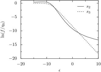
Figure 5: Comparing $f_{3}(\epsilon)$ to $f_{2}(\epsilon)$ which was derived using Eq. (32). The two functions are unequal proving that the $s_{3}$ state is different from the $s_{2}$ state.

4 The Information-theory approach to violent relaxation and its relation to the LB67 theory

Recently, a new approach to violent relaxation was proposed in a interesting paper by T. K. Nakamura (Nakamura, 2000). In that paper, Nakamura uses an information-theory approach (Jaynes, 1957a, b) to define the entropy of a collisionless system and thereby find its equilibrium state. Nakamura’s theory (hereafter NK00) predicts a different equilibrium state than LB67, and it is therefore interesting to check weather his theory is transitive or not. We will not, however, try to answer the question which one of these theories is more correct as it is, in our opinion, still an open question. Instead, we shall first give a brief description of NK00 and its main results, and then re-derive it theory using a combinatorial approach which would enable us to compare it with the LB67 theory, and point to the reasons of why they differ. Finally we will analyse the two-levels configuration which goes into the water-bag configuration in a limiting case. The result of this analysis will be used in the next section when we examine the transitivity of the NK00 theory in a double relaxation experiment.

4.1 An outline of the NK00 theory

In the NK00 theory we adopt the probabilistic description of the phase-space density $f(t,\mathbf{r},\mathbf{v})$. Let $f_{0}(\mathbf{r},\mathbf{v})$ be the initial phase-space density of the system, and define the initial probability distribution $p_{0}(\mathbf{r},\mathbf{v})$ for finding a (single) test point at $t=0$ by

$$p_{0}(\mathbf{r},\mathbf{v})=\frac{1}{M}f_{0}(\mathbf{r},\mathbf{v})\ .$$ (33)

Then we let the test point move under gravity just like any phase-space element, and we define the probability distribution $p(\mathbf{r},\mathbf{v},t)$ as the probability distribution of finding the test point at time $t>0$. The conservation of phase-space volume guarantees that $p(\mathbf{r},\mathbf{v},t)=f(\mathbf{r},\mathbf{v},t)/M$ for all $t>0$.

Next, we divide phase-space into macro-cells $i=1,2,3,\ldots$ of volume $\tilde{\omega}$, and define the coarse-grained probability $\bar{p}_{i}$ as the probability of finding the point in the $i$’th macro-cell when the system reaches an equilibrium. From the above discussion it is clear that $\bar{p}_{i}$ is equal to $\bar{f}_{i}/M$ with $\bar{f}_{i}$ being the coarse-grained DF in the macro-cell $i$ at equilibrium.

To calculate $\bar{p}_{i}$ using the information-theory approach, we define the joint probability-distribution $p_{i}(\mathbf{r},\mathbf{v})$ which measures the probability of initially finding the test point at the $(\mathbf{r},\mathbf{v})$ and later at the macro-cell $i$. Then we maximise the Shanon entropy

$$S=-\sum_{i}\int\!\!d^{6}\tau p_{i}(\mathbf{r},\mathbf{v})\log p_{i}(\mathbf{r},\mathbf{v})\ ,$$ (34)

subject to constraints of energy conservation, phase-space volume conservation and initial conditions. The resultant distribution can be best written in terms of the conditional probability $K_{i}(\mathbf{r},\mathbf{v})=p_{i}(\mathbf{r},\mathbf{v})/p_{0}(\mathbf{r},\mathbf{v})$:

$$K_{i}(\mathbf{r},\mathbf{v})=e^{-\beta\epsilon_{i}-\delta(\mathbf{r},\mathbf{v})-\lambda_{i}/p_{0}(\mathbf{r},\mathbf{v})}\ ,$$ (35)

with $\epsilon_{i}$ being the energy per unit mass of the macro-cell $i$, and $\beta,\delta(\mathbf{x},\mathbf{v}),\lambda_{i}$ are the Lagrange multipliers, to be found from the energy conservation constraint, from the initial conditions

$$\sum_{i}K_{i}(\mathbf{r},\mathbf{v})=1\ ,$$ (36)

and from the phase-space volume conservation constraint

$$\int\!\!K_{i}(\mathbf{r},\mathbf{v})\,d^{6}\tau=\tilde{\omega}\ .$$ (37)

From Eqs. (35-37) it is evident that the dependence of $K_{i}(\mathbf{r},\mathbf{v})$ on the indices $i,\mathbf{r},\mathbf{v}$ is only via $\epsilon_{i}$ and $p_{0}(\mathbf{r},\mathbf{v})$, the latter can be trivially be replaced by $f_{0}(\mathbf{r},\mathbf{v})$. Therefore, the above equations can be re-written using the $K(\epsilon,\eta)$ function, together with the $\tau(\eta)$ and $g(\epsilon)$ functions which were defined in Sec. 3.1:

$$K(\epsilon,\eta) = (\tilde{\omega})^{-1}e^{-\beta\epsilon-\delta(\eta)-\lambda(\epsilon)/\eta}\ ,$$ (38)

$$\int_{\Phi(0)}^{\infty}\!\!g(\epsilon)K(\epsilon,\eta)\,d\epsilon = 1\ ,$$ (39)

$$\int_{0}^{\infty}\!\!\tau(\eta)K(\epsilon,\eta)\,d\eta = 1\ .$$ (40)

The coarse-grained equilibrium DF is then given by

$$f(\epsilon)=\int_{0}^{\infty}\!\!\tau(\eta)\eta K(\epsilon,\eta)\,d\eta\ .$$ (41)

As noted by Nakamura, a prominent difference between his result and the LB67 results is that in the non-degenerate limit his expression reduces to a single Maxwellian distribution, whereas the LB67 expression is a superposition of Maxwellian distributions with different dispersions. This difference can be attributed to the fact that in LB67 we discretise phase-space using phase-space elements of equal volume and different masses, while, as we shall see below, the NK00 theory can be derived by discretising phase-space using elements of equal mass, which are associated with different phase-space volumes.

Another evident difference comes from the phase-space volume conservation constraint Eq. (36). This constraint guarantees that the total phase-space volume of all phase-space patches that ended up in macro-cell $i$ will be equal to the macro-cell volume. Consequently the total phase-space volume of the initial system $\int_{0}^{\infty}\!\!\tau(\eta)\,d\eta$ must be equal to the total phase-space volume of the non-vanishing phase-space density in the equilibrium configuration. This constraint does not exist in the LB67 theory where the macro-cells can be only partly full - as is the case, for example, in the non-degenerate equilibrium of a system which is initially in the water-bag configuration. Furthermore, this can not be trivially changed by adding a volume of zero phase-space density to the initial condition, because setting $p(\mathbf{r},\mathbf{v})=0$ would lead to divergences in Eq. (35). In Sec. 4.3 we shall see how this problem can be overcome by using a limiting procedure.

4.2 Deriving the NK00 theory in a combinatorial approach

To derive the NK00 theory in a combinatorial approach, we realise the phase-space density distribution using $N\gg 1$ elements of equal mass $m$. As in Sec. 3.1, we assume that initially the system is made of a discrete set of density levels $\eta_{1},\eta_{2},\ldots$ occupying phase-space volumes $V_{1},V_{2},\ldots$. Then the overall number of elements that realise a phase-space density $\eta_{J}$ is $N_{J}=V_{J}\eta_{J}/m$.

Next, we let the system reach an equilibrium through the process of violent relaxation, and divide phase-space into macro-cells of equal volume $\tilde{\omega}$, which are label by the index $i=1,2,\ldots$. We define a micro-state by specifying the macro-cell in which every element ended up. A macro-state is then defined by the matrix $\{n_{iJ}\}$ which counts how many elements that initially realised the density level $\eta_{J}$ ended up in the macro-cell $i$. Using $\{n_{iJ}\}$, the coarse-grained DF at macro-cell $i$ is given by

$$\bar{f}_{i}=\frac{m}{\tilde{\omega}}\sum_{J}n_{iJ}\ .$$ (42)

Finally, we define the function $W\big{(}\{n_{iJ}\big{)}$ which counts how many micro-states give the macro state $\{n_{iJ}\}$. It is then a simple combinatorics to show that

$$W\big{(}\{n_{iJ}\}\big{)}=\prod_{J}\frac{N_{J}!}{\prod_{i}n_{iJ}!}\ .$$ (43)

Let us pause here and explain that this rather simple formula is a result of the way we define a micro-state - by specifying the macro-cell in which each element is found. We do not care exactly how the different elements are distributed in each macro-cell. A different approach, in which the macro-cells can be only partly full, and the distribution of the different elements in a macro-cell is taken into account when defining a micro-state, was taken by Kull et al (1997). It is not difficult to see that when one adds the constraint that all macro-cells must be completely full to their theory, Nakamura’s results are recovered. This is because in such case the number of different ways to arrange the different elements in the macro-cell is independent of which elements we are organising - as long as the macro-cell is completely full. Therefore the number of micro-states in a macro-state would be proportional to Nakamura’s $W\big{(}\{n_{iJ}\}\big{)}$, and consequently the equilibrium state would be identical in both theories.

Next, we use $W\big{(}\{n_{iJ}\}\big{)}$ to define the entropy

$$S\equiv\log W\simeq const-\sum_{i,J}n_{iJ}(\log n_{iJ}-1)\ ,$$ (44)

where in the second equality we have used Stirling’s formula to approximate $\log(n_{iJ}!)\simeq n_{iJ}(\log n_{iJ}-1)$.

Before maximising the entropy to find the most probable macro-state, we first write down the constraints on $\{n_{iJ}\}$. The first constraint comes from the initial conditions

$$\sum_{i}n_{iJ}=N_{J}=\frac{V_{J}\eta_{J}}{m}\ .$$ (45)

Then we have the phase-space volume conservation constraint, ensuring that the total phase-space volume that is carried by elements that ended up in the macro-cell $i$ will be exactly $\tilde{\omega}$, or, in other words, that each macro-cell is completely filled:

$$\sum_{J}n_{iJ}\frac{m}{\eta_{J}}=\tilde{\omega}\ .$$ (46)

The last constraint is the energy constraint

$$\sum_{i}\tilde{\omega}\bar{f}_{i}\left[\frac{1}{2}v_{i}^{2}-\frac{1}{2}G\sum_{j}\frac{\tilde{\omega}\bar{f}_{j}}{|r_{i}-r_{j}|}\right]=E\ ,$$ (47)

where $r_{i}$ and $v_{i}$ are the mean position and velocity of the $i$’th macro-cell.

To maximise the entropy under the above constraint we use Lagrange multipliers. The function that we wish to maximise with respect to $n_{iJ}$ is therefore

$$I=S-\sum_{J}\lambda_{i}n_{iJ}-\sum_{i}\delta_{J}n_{iJ}-\beta E\ .$$ (48)

Differentiating $I$ with respect to $n_{iJ}$ and equating it to zero, we get

$$\frac{dI}{dn_{iJ}}=-\log n_{iJ}-\delta_{J}-\frac{\lambda_{i}}{\eta_{J}}-\beta m\epsilon_{i}=0\ ,$$ (49)

with $\epsilon_{i}=v_{i}^{2}/2+\Phi(r_{i})$ as usual, and therefore

$$n_{iJ}=e^{-\beta m\epsilon_{i}-\delta_{J}-\frac{\lambda_{i}}{\eta_{J}}}\ .$$ (50)

Finally, we pass to a continuous description by giving every initial phase-space density level a small width $\Delta\eta$. Then using the $\tau(\eta)$ and $g(\epsilon)$ function we replace

$$\sum_{J} \to \frac{1}{\Delta\eta}\int\!\!d\eta\ ,$$ (51)

$$\sum_{i} \to \frac{1}{\tilde{\omega}}\int\!\!d\epsilon\,g(\epsilon)\ ,$$ (52)

$$V_{J} \to \Delta\eta\tau(\eta_{J})\ ,$$ (53)

$$n_{iJ} \to \frac{\Delta\eta\tilde{\omega}}{m}\,\tau(\eta_{J})\eta_{J}K(\epsilon_{i},\eta_{J})\ .$$ (54)

Plugging these replacements into Eqs. (50, 45, 46) and redefining $m\beta\to\beta$, we recover the NK00 Eqs. (38, 39, 40).

This combinatorial formulation of the NK00 theory is very much along the lines of ordinary statistical mechanic of a classical Boltzmann gas. Indeed, if we replace the notion of phase-elements with particles of equal mass and discard the constraint of conservation of phase-space volume Eq. (40), we have a text-book derivation of the Boltzmann gas statistics. It is therefore not surprising that Nakamura found that his equilibrium DF reduces to the well-known Maxwell-Boltzmann distribution in such case. We do not agree, however, with Nakamura’s claim that this property is a proof for its correctness over the LB67 theory. This is because a collisionless relaxation is essentially a very different process from the collision-full relaxation that occurs in Boltzmann gas, driven by different physical processes over different timescales. However, as previously mentioned, deciding which theory is more correct is not the goal of this paper.

4.3 Analysing the two-levels configuration

As was noted in the end of Sec. 4.1, the NK00 theory cannot handle a zero phase-space density directly. Therefore it is not straightforward to analyse the equilibrium state that results from an initial water-bag configuration, as in this configuration there is one patch of phase-space density $\eta_{0}$ surrounded by an infinite volume of zero phase-space density. The way this can be done is to consider an initial state with two density levels $\eta_{0}$ and $\eta_{1}$ with corresponding volumes $V_{0}$ and $V_{1}$. The water-bag configuration is then recovered by taking the limit $\eta_{1}\to 0,V_{1}\to\infty$ and $\eta_{1}V_{1}\to 0$.

To derive the equilibrium configuration of the two-levels system we use the fact that in this particular case the matrix $\{n_{iJ}\}$ can be expressed in terms of $\bar{f}_{i}$, thereby greatly simplifying the end result. Let us then re-derive the equilibrium equation for this particular case instead of using Eqs. (38-41). Denoting by $n_{i,0}$ and $n_{i,1}$ the total number of elements of $\eta_{0}$ and $\eta_{1}$ that end-up in the $i$’th macro-cell, the coarse-grained DF is given by

$$\bar{f}_{i}=\frac{m}{\tilde{\omega}}(n_{i,0}+n_{i,1})\ .$$ (55)

Then using the conservation of phase-space volume constraint (46),

$$n_{i,0}\frac{V_{0}}{N_{0}}+n_{i,1}\frac{V_{1}}{N_{1}}=\tilde{\omega}\ ,$$ (56)

with $N_{0},N_{1}$ being the total number of elements with densities $\eta_{0},\eta_{1}$, given by Eq. (45), we express $n_{i,0}$ and $n_{i,1}$ in terms of $\bar{f}_{i}$:

$$n_{i,0} = \frac{\tilde{\omega}}{m}\frac{\bar{f}_{i}-\eta_{1}}{\eta_{0}-\eta_{1}}\eta_{0}\ ,$$ (57)

$$n_{i,1} = \frac{\tilde{\omega}}{m}\frac{\eta_{0}-\bar{f}_{i}}{\eta_{0}-\eta_{1}}\eta_{1}\ .$$ (58)

The energy constraint is given by Eq. (47), and the initial-condition constraint is

$$\sum_{i}n_{i,0}=N_{0}=\frac{\eta_{0}V_{0}}{m}\ .$$ (59)

Notice that we need only the $N_{0}$ constraint since the $N_{1}$ constraints follows directly from requiring that the total phase-space volume occupied by the equilibrium system would be equal to $V=V_{0}+V_{1}$. In fact, instead of Eq. (59), we can use an alternative total mass constraint, provided that the overall phase-space volume is conserved. This is done as follows: expressing $n_{i,0}$ in terms of $\bar{f}_{i}$ in Eq. (59) we get

$$\tilde{\omega}\sum_{i}\frac{\bar{f}_{i}-\eta_{1}}{\eta_{0}-\eta_{1}}=V_{0}\ ,$$ (60)

which gives us

$$\sum_{i}\tilde{\omega}\bar{f}_{i}-\eta_{1}\sum_{i}\tilde{\omega}=V_{0}\eta_{0}-V_{1}\eta_{1}\ .$$ (61)

But $\sum_{i}\tilde{\omega}=V_{0}+V_{1}$ (conservation of total phase-space volume) and therefore we find

$$\sum_{i}\tilde{\omega}\bar{f}_{i}=V_{0}\eta_{0}+V_{1}\eta_{1}=M\ .$$ (62)

Adding these constraints together with the appropriate Lagrange multipliers to the entropy, the expression that we need to maximise is

$$I \simeq const-\sum_{i}n_{i,0}\big{(}\log n_{i,0}-1\big{)}$$ (64)

$$-\sum_{i}n_{i,1}\big{(}\log n_{i,1}-1\big{)}+\tilde{\beta}E+\tilde{\mu}\sum_{i}\tilde{\omega}\bar{f}_{i}\ .$$

Differentiating $I$ with respect to $\bar{f}_{i}$ and equating to $0$ we find

$$-\frac{\eta_{0}}{\eta_{0}-\eta_{1}}\frac{\tilde{\omega}}{m}\log\left(\frac{\tilde{\omega}}{m}\frac{\bar{f}_{i}-\eta_{1}}{\eta_{0}-\eta_{1}}\eta_{0}\right)$$ (65)

$$+\frac{\eta_{1}}{\eta_{0}-\eta_{1}}\frac{\tilde{\omega}}{m}\log\left(\frac{\tilde{\omega}}{m}\frac{\eta_{0}-\bar{f}_{i}}{\eta_{0}-\eta_{1}}\eta_{1}\right)+\tilde{\beta}\tilde{\omega}\epsilon_{i}+\tilde{\mu}\tilde{\omega}=0\ .$$ (66)

After a trivial algebra and redefinition of the Lagrange multipliers $\tilde{\beta}$ and $\tilde{\mu}$ to $\beta$ and $\mu$, we obtain

$$\frac{\frac{\bar{f}_{i}-\eta_{1}}{\eta_{0}-\eta_{1}}}{\left(\frac{\eta_{0}-\bar{f}_{i}}{\eta_{0}-\eta_{1}}\right)^{\eta_{1}/\eta_{0}}}=e^{-\beta(\epsilon_{i}-\mu)}\ .$$ (67)

Notice how the denominator provides an upper cut-off for $\bar{f}_{i}$, as it forbids it from exceeding $\eta_{0}$.

Consider now the $\eta_{1}\to 0$ limit. Seemingly, it would go into an isothermal sphere

$$\bar{f}_{i}=\eta_{0}e^{-\beta(\epsilon_{i}-\mu)}\ ,$$ (68)

but this is not the case as for every finite $\eta_{1}$, $\bar{f}_{i}$ cannot exceed $\eta_{0}$. It is easy to see that the right limit is therefore

$$f_{NK}(\epsilon)=\left\{\begin{array}[]{lcl}\eta_{0}&,&\epsilon<\mu\\ \eta_{0}e^{-\beta(\epsilon-\mu)}&,&\epsilon\geq\mu\end{array}\right.\ .$$ (69)

This distribution is not the LB67 Fermi-Dirac distribution given by Eq. (16) or Eq. (17), but is what corresponds to that distribution on the NK00 theory. It is not smooth, and is exactly isothermal for energies $\epsilon>\mu$.

For the water-bag model in LB67 the condition that no two elements of phase-density can overlap leads to a statistics with exclusion, equivalent to the Fermi-Dirac problem. It is not clear to us how Nakamura’s formulation could obtain the Fermi-Dirac statistics.

5 Non-transitivity in the Nakamura theory of violent relaxation

Having found the equilibrium configuration of the water-bag initial configuration in the NK00 theory, we are in a position to test the theory’s transitivity. The procedure for that is identical to the one that was used in the LB67 case, in sections 3.2, 3.3, and therefore will not be repeated. Instead, we shall first describe how the $s_{1}$ and $s_{3}$ configurations are found and then how $s_{2}$ is compared to the $s_{3}$ configuration.

To find the $s_{1}$ and $s_{3}$ configurations, we must first find the gravitational potential of the DF in Eq. (69) in a sphere of radius $R$, and then fix $\beta$ and $\mu$ so that the overall energy and mass will be equal to $E$ and $M$. Additionally, just as in the LB67 case, we assume that the final equilibrium state is spherical and therefore the Poisson equation for $\Phi(r)$ is:

$$\frac{1}{r^{2}}\frac{d}{dr}\left(r^{2}\frac{d\Phi}{dr}\right)=(4\pi)^{2}G\int_{0}^{\infty}v^{2}f_{NK}\big{[}v^{2}/2+\Phi(r)\big{]}\,dv\ .$$ (70)

Passing from $\Phi(r)$ to the dimensionless $\psi(r)$ by

$$\psi(r)\equiv\beta[\mu-\Phi(r)]\ ,$$ (71)

Eq. (70) simplifies to

$$-\frac{1}{\beta r^{2}}\frac{d}{dr}\left(r^{2}\frac{d\psi}{dr}\right)=(4\pi)^{2}G\eta_{0}$$ (72)

$$\times\int_{0}^{\infty}\!\!v^{2}\,dv\left\{\begin{array}[]{lcl}1&,&\beta v^{2}/2<\psi(r)\\ e^{\psi(r)}e^{-\beta v^{2}/2}&,&\beta v^{2}/2\geq\psi(r)\end{array}\right.$$ (75)

Finally, changing variables $r\to x$

$$x\equiv\left(\frac{16\pi^{2}\sqrt{2}G\eta_{0}}{\beta^{1/2}}\right)^{1/2}r\ ,$$ (76)

and using the Error-function $\mbox{erf}(x)=\frac{2}{\sqrt{\pi}}\int_{0}^{x}e^{-t^{2}}dt$, the ordinary differential equation for $\psi(x)$ is

$$-\frac{1}{x^{2}}\frac{d}{dx}\left(x^{2}\frac{d\psi}{dx}\right)=I(\psi)\ ,$$ (77)

with

$$I(\psi)=\left\{\begin{array}[]{lcl}\frac{\sqrt{\pi}}{2}e^{\psi}&,&\psi<0\\ \frac{2}{3}\psi^{3/2}+\sqrt{\psi}+\frac{\sqrt{\pi}}{2}e^{\psi}\left(1-\mbox{erf}\sqrt{\psi}\right)&,&\psi\geq 0\end{array}\right.\ .$$ (80)

To integrate this equation we must first set its initial condition. We let $\psi(0)=\psi_{0}$ be a free parameter, and $\psi^{\prime}(0)=0$ since in a spherical system the gravitational force vanishes in the centre. Then once $\psi(x)$ is (numerically) found, we fix $\mu$ by requiring that $\Phi(R)=-GM/R$. This way we can find the gravitational potential, and thereafter the total mass and energy for any given $\beta$ and $\psi_{0}$. The last step is to find the right $\beta$ and $\psi_{0}$ that would give us $M$ and $E$.

Practically, instead of looking for $\beta$, $\psi_{0}$ for a specific $E$ and $M$ choice in $s_{1}$ and $s_{3}$, we have picked two different values of $\beta$ and and two corresponding values of $\psi_{0}$ to satisfy the total mass constraint. Once $\psi_{0}$ is fixed it also defines a total energy. We chose $\beta_{1}>\beta_{3}$ in order to obtain $E_{1}<E_{2}$.

Let us now see how the $s_{2}\leftrightarrow s_{3}$ comparison can be done. According to Sec. 4, $f_{2}(\epsilon)$ is determined by the following set of equations:

$$K(\epsilon,\eta) = (\tilde{\omega})^{-1}e^{-\beta_{2}\epsilon-\delta(\eta)-\lambda(\epsilon)/\eta}\ ,$$ (81)

$$1 = \int_{\Phi_{2}(0)}^{\infty}g_{1}(\epsilon)K(\epsilon,\eta)\,d\epsilon\ ,$$ (82)

$$1 = \int_{0}^{\eta_{0}}\tau_{1}(\eta)K(\epsilon,\eta)\,d\eta\ ,$$ (83)

$$f_{2}(\epsilon) = \int_{0}^{\eta_{0}}\tau_{1}(\eta)\eta K(\epsilon,\eta)\,d\eta\ .$$ (84)

Additionally, we know that $f_{3}(\epsilon)$ is given by

$$f_{3}(\epsilon)=\left\{\begin{array}[]{lcl}\eta_{0}&,&\epsilon<\mu_{3}\\ \eta_{0}e^{-\beta_{3}(\epsilon-\mu_{3})}&,&\epsilon\geq\mu_{3}\end{array}\right.\ ,$$ (85)

and $g_{3}(\epsilon)$, $\Phi_{3}(r)$ have been found as described above. Assuming that $s_{2}=s_{3}$, we replace these functions with $f_{2}(\epsilon),g_{2}(\epsilon)$ and $\Phi_{2}(\epsilon)$ in Eqs. (82-84), and differentiate Eq. (84) with respect to $\epsilon$. Using Eq. (83) we get

$$f^{\prime}_{3}(\epsilon)=-\beta_{2}f_{3}(\epsilon)-\lambda^{\prime}(\epsilon)\ ,$$ (86)

and therefore

$$\lambda(\epsilon)=C+\beta_{2}\int_{\epsilon}^{\infty}f_{3}(\epsilon^{\prime})d\epsilon^{\prime}-f_{3}(\epsilon)\equiv C+\lambda_{0}(\epsilon)\ ,$$ (87)

with $C$ some unknown integration constant. The integral in $\lambda_{0}(\epsilon)$ can be done analytically, yielding

$$\lambda_{0}(\epsilon)=\left\{\begin{array}[]{lcl}\eta_{0}\left[\frac{\beta_{2}}{\beta_{3}}-1+\beta_{2}(\mu_{3}-\epsilon)\right]&,&\epsilon<\mu_{3}\\ \eta_{0}\left(\frac{\beta_{2}}{\beta_{3}}-1\right)e^{-\beta_{3}(\epsilon-\mu_{3})}&,&\epsilon\geq\mu_{3}\end{array}\right.\ .$$ (88)

Then from Eq. (82) we find that

$$e^{\delta(\eta)} = e^{-C/\eta}(\tilde{\omega})^{-1}\int_{\Phi_{3}(0)}^{\infty}\!\!g_{3}(\epsilon)e^{-\beta_{2}\epsilon-\lambda_{0}(\epsilon)/\eta}\,d\epsilon$$

$$\equiv e^{-C/\eta}(\tilde{\omega})^{-1}D_{0}(\eta)\ ,$$

and therefore

$$K(\epsilon,\eta) = (\tilde{\omega})^{-1}e^{-\beta_{2}\epsilon-\delta(\eta)-\lambda(\epsilon)/\eta}$$ (90)

$$= \frac{e^{-\beta_{2}\epsilon-\lambda_{0}(\epsilon)/\eta}}{D_{0}(\eta)}\ .$$ (91)

Notice how the unknown integration constant $C$ and the dimensional constant $\tilde{\omega}$ are cancelled out.

Next we calculate $f_{2}(\epsilon)$ using Eq. (84) and fix $\beta_{2}$ such that the energy of the system is $E+\Delta E$. Once $\beta_{2}$ is fixed, $K(\epsilon,\eta)$ is completely resolved in terms of $s_{1}$ and $s_{3}$ functions, and we can check if it solves the maximum-entropy equations by plugging it into Eq. (83).

Finally, we should note that as in the LB67 case, the $\tau_{1}(\eta)$ function has a strong peak at $\eta=\eta_{0}$ due to the degeneracy. Here, however, this peak is proportional to $\delta(\eta-\eta_{0})$ as $f_{1}(\epsilon)=\eta_{0}$ for every $\Phi_{1}(0)<\epsilon<\mu_{1}$. The prefactor in front of this delta function is $V_{deg}$ - the volume of phase-space for which $\Phi_{1}(0)<\epsilon<\mu_{1}$, which can be easily calculated from Eq. (30). Therefore, to preform the integration over $\tau_{1}(\eta)$ in Eqs. (83, 84) numerically, we first calculate the smooth contribution which comes from the $\tau_{1}(\eta)$ with $\eta<\eta_{0}$, and then add the delta-function contribution by evaluating the integrands at $\eta=\eta_{0}$ and multiplying them by $V_{deg}$.

5.1 Numerical results

As in the LB67 case, the $s_{0}$ state was constructed as a water-bag configuration with $\eta$ given by Eq. (15) and $M=1$, $R=1$, $G=1$. The $s_{1}$ and $s_{3}$ configurations were then chosen as described in the previous sub-section, by fixing $\beta$ and varying $\psi_{0}$ until the total mass constraint was satisfied. The main numerical parameters of these configurations are summarised in Table 2.

Table 2: The numerical parameters that specify the $s_{1}$ and $s_{3}$ states in NK00 double relaxation experiment. $E$ is the total energy, $\beta$ and $\mu$ are the Lagrange multipliers in Eq. (69), and $\Phi(0)$ is the gravitational potential at $r=0$.

State	$E$	$\beta$	$\mu$	$\Phi(0)$
$s_{1}$	$-6.405$	$3.0$	$-15.30$	$-35.08$
$s_{3}$	$-4.306$	$0.68$	$-14.08$	$-27.80$

Figure 6 shows the density profiles of the $s_{1}$ and $s_{3}$ configuration. As expected, the hotter system, $s_{3}$, has a core with a lower density than the $s_{1}$ system. Figure 7 shows the DF of these systems, and Fig. 8 compares the $M(V)$ functions of these two states, showing that $M_{3}(V)\leq M_{1}(V)$ for every $V$ - and therefore the transition $s_{1}\to s_{3}$ is allowed.

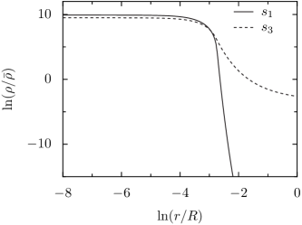
Figure 6: Density profiles of the $s_{1}$ and $s_{3}$ states in the double-relaxation experiment of the NK00 theory. $\bar{\rho}$ is the average density given by $\bar{\rho}=3M/(4\pi R^{3})$. As in Fig. 1, the $s_{3}$ state corresponds to a hotter system with higher energy which makes it less concentrated.

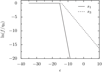
Figure 7: DFs of $s_{1}$ and $s_{3}$ in the NK00 experiment. The functional form of these DFs is given in Eq. (69) and Table. 2. Unlike the Fermi-Dirac DFs of the LB67 theory given in Fig. 2, these DFs have a sharp transition between a completely degenerate core with $f=\eta_{0}$ for $\epsilon<\mu$ to an isothermal envelope for $\epsilon\geq\mu$.

Figure 8: The $M(V)$ functions of $s_{1}$ and $s_{3}$ in the double-relaxation experiment of the NK00 theory. $M_{0}$ and $V_{0}$ are defined as in Fig. 3, but here the $y$-axis is $M/M_{0}$ whereas in Fig. 8 is $\ln(M/M_{0})$. This is because the range over which $M/M_{0}$ varies is much smaller than that of the NK00 case. Nevertheless, as in Fig. 3, $M_{3}(V)\leq M_{1}(V)$ for every $V$, showing that $s_{3}$ is more mixed than $s_{1}$.

Finally, to compare the $s_{2}$ configuration to the $s_{3}$ configuration we have varied $\beta_{2}$ in the range $0.1<\beta_{2}<100$ until we obtained $E_{2}=E_{3}=-4.306$ with $\beta_{2}=0.6944$. This was the only solution in that range, and we believe that it is the only physical solution in general. The graph of $E_{2}(\beta)$ verses $E_{3}$ in the range $[0.1,4]$ is shown in Fig. 9.

Once $\beta_{2}$ was found, we used the expression of $K(\epsilon,\mu)$ in Eq. (5), to calculate the RHS of Eq. (83) and compare it to $1$. Figure 10 shows this comparison. The disagreement between the RHS and $1$ is sometimes as high as 3 orders of magnitude - much higher than any possible numerical error. We therefore conclude that also the NK00 theory is non-transitive.

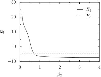
Figure 9: The energy $E_{2}$ of $s_{2}$ as a function of $\beta_{2}$, together with the energy $E_{3}=-4.306$. The value of $\beta_{2}$ for which the two energies agree is $\beta_{2}=0.6944$. No other solutions were founds for $\beta_{2}$ up to $100$, and we therefore believe that this is the only physical solution.

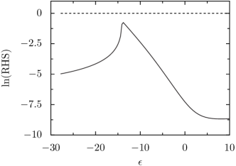
Figure 10: Comparing the RHS of Eq. (40) to its LHS (in natural logarithmic scale). The two sides of the equations are in gross disagreement, proving that also the NK00 theory is non-transitive.

6 Conclusions

In this paper we have demonstrated that the statistic-mechanical theories of violent relaxation by Lynden-Bell and Nakamura are both non-transitive. This non-transitivity is a result of the phase-mixing that occurs when the system relaxes; as the fine-grained phase-space density filaments become thiner and thiner, the system is better described in terms of the coarse-grained phase-space density. Any further relaxation of the system should be therefore considered in terms of the coarse-grained phase-space density - which as we have seen would yield different results from a prediction that is based on the initial fine-grained phase-space density. This is a worrying aspect of these theories as it is easy to imagine a scenario where part of the system mixes, then fluctuates, and then mixes once again. The predictions of the theory, based on the fine-grained density, will then give us a wrong result.

In some sense we have been breaking into an open door. Even without considering the non-transitivity of the theories, they are plagued by severe problems. There exist two equally plausible ways of discretising phase-space, one with equal volume elements and one with equal mass elements, which yield two different results. More importantly, the ability of the theories to predict the final outcome of a violent-relaxation process is very limited. Indeed, as was mentioned in Sec. 2, the most important reason for this is that violent-relaxation is almost never complete; the fluctuations of the gravitational potential die much faster for the system to settle in the most probable state.

Nevertheless, we believe that these difficulties and ambiguities in exactly how to do the statistical mechanics of the collisionless Boltzmann equation teach us an important lesson. The non-transitivity that we have shown is a sign that a kinetic description of violent relaxation is probably incomplete, as the equilibrium is dependent on the evolutionary path of the system. Instead, what is probably needed is a dynamical approach to the problem. Indeed most of the above difficulties are circumvented if instead of aiming to derive a universal most probable state, we reduce our aim to that of finding an appropriate and useful evolution equation for the coarse-grained $\bar{f}$.

An interesting attempt to find such equation was taken by Chavanis (1998), who used the maximal entropy-production principle (MEPP) to obtain a close equation for $\bar{f}$. His analysis, however, uses the initial fine-grained $\tau(\eta)$ to define the (Lynden-Bell) entropy rather than the instantaneous, coarse-grained $\tau(\bar{\eta})$, which according to the above discussion is more correct. Derivation of a useful dynamical equation for $\bar{f}$ thus remains a challenging open problem.

References

- Binney (2004) Binney J., 2004, MNRAS, 350, 939
- Chavanis & Sommeria (1998) Chavanis P.-H., Sommeria J., 1998, MNRAS, 296, 569
- Chavanis (1998) Chavanis P.-H., 1998, MNRAS, 300, 981
- Jaynes (1957a) Jaynes E. T., 1957, Phys. Rev., 106, 620
- Jaynes (1957b) Jaynes E. T., 1957, Phys. Rev., 108, 171
- Hénon (1968) Hénon M., 1968, Bull. Astronomique, 3, 241
- Lynden-Bell (1967) Lynden-Bell D., 1967, MNRAS, 136, 101
- Lynden-Bell & Lynden-Bell (1999a) Lynden-Bell D., Lynden-Bell R. M., 1999a, Proc. R. Soc. A, 455, 475
- Lynden-Bell & Lynden-Bell (1999b) Lynden-Bell D., Lynden-Bell R. M., 1999b, Proc. R. Soc. A, 455, 3261
- Lynden-Bell & Lynden-Bell (2004) Lynden-Bell D., Lynden-Bell R. M., 2004, J. Stat. Phys, in press, (cond-mat/0401093)
- Kull et al (1997) Kull A., Treumann R. A., Bohringer H, 1997, ApJ, 484, 58
- Nakamura (2000) Nakamura T. K. 2000, ApJ, 531, 739
- Navarro, Frenk & White (1995) Navarro J. F., Frenk C. S., White S. D. M, 1995, MNRAS, 275, 720
- Navarro, Frenk & White (1996) Navarro J. F., Frenk C. S., White S. D. M, 1996, ApJ, 462, 563
- Navarro, Frenk & White (1997) Navarro J. F., Frenk C. S., White S. D. M, 1997, ApJ, 490, 493
- Tremaine, Hénon & Lynden-Bell (1986) Tremaine S., Hénon M., Lynden-Bell D., (1986), MNRAS, 219, 285