Diffuse X-rays from the Arches and Quintuplet Clusters

Abstract

The origin and initial mass function of young stellar clusters near the Galactic center are still poorly understood. Two of the more prominent ones, the Arches and Quintuplet clusters, may have formed from a shock-induced burst of star formation, given their similar age and proximity to each other. Their unusual mass distribution, however, may be evidence of a contributing role played by other factors, such as stellar capture from regions outside the clusters themselves. Diffuse X-ray emission from these sources provides us with a valuable, albeit indirect, measure of the stellar mass-loss rate from their constituents. Using recent data acquired with Chandra, we can study the nature and properties of the outflow to not only probe the pertinent physical conditions, such as high metallicity, the magnetic field, and so forth, but also to better constrain the stellar distribution within the clusters, in order to identify their formative history. In this paper, we present a set of three-dimensional smoothed particle hydrodynamics simulations of the wind-wind interactions in both the Arches and Quintuplet clusters. We are guided primarily by the currently known properties of the constituent stars, though we vary the mass-loss rates in order to ascertain the dependence of the measured X-ray flux on the assumed stellar characteristics. Our results are compared with the latest observations of the Arches cluster. Our analysis of the Quintuplet cluster may be used as a basis for comparison with future X-ray observations of this source.

1 Introduction

Understanding the environment’s role in star formation and, in turn, the feedback exerted by star formation on the Galactic environment, is a problem of significance to several fields in astronomy, from the creation of compact objects to the formation of galaxies. The Galactic center, with its relatively high magnetic field strength, clouds with high particle density, and large velocity dispersions, provides an ideal environment to study star formation under extreme conditions (Morris, 1993; Melia & Falcke, 2001). This type of investigation can benefit from the existence of several stellar clusters in this region, including the Arches and Quintuplet clusters. Learning more about their stellar constituents, and possibly their formative history, may even give us a glimpse into the emergence of objects that will ultimately populate the central parsec of the Galaxy (e.g., Gerhard, 2001; McMillan & Portegies Zwart, 2003).

The Arches and Quintuplet clusters have been studied over a range of wavelengths, from radio to X-ray. X-rays provide a unique window for investigating both the formation of binaries (point sources from binary interactions) and the wind interactions within the entire cluster (diffuse emission). As Rockefeller et al. (2004) have shown, the diffuse X-ray emission is a sensitive measure of the mass-loss rate of stars in mutually interactive situations. Stellar mass-loss remains one of the largest uncertainties in stellar evolution (e.g., Wellstein & Langer, 1999). X-ray observations of these clusters represent a unique probative tool for studying the winds produced by high-metallicity systems.

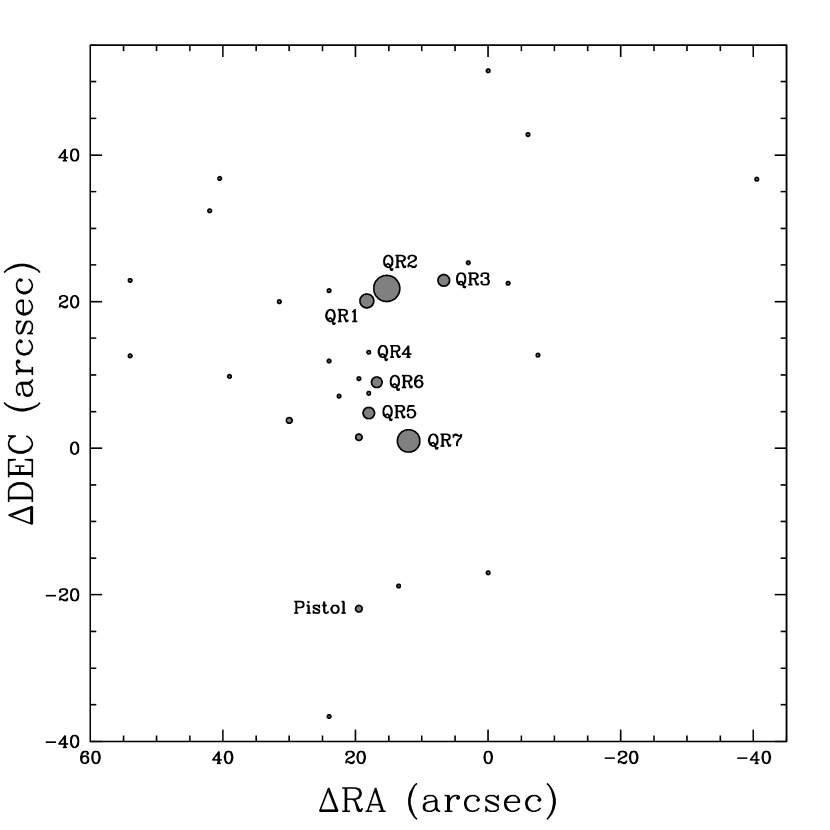
Figure 2: Location of the 31 wind-producing stars used in the simulations of the Quintuplet cluster, relative to $\alpha(1950)$: $17^{h}\,43^{m}\,4.5^{s}$, $\delta(1950)$: $-28^{\circ}\,48^{\prime}\,35^{\prime\prime}$ (Lang et al., 1999). The radius of each circle corresponds (on a linear scale) to that star’s mass loss rate. Setting the scale is QR2, with $\dot{M}=1.5\times 10^{-4}\;M_{\odot}$ yr^-1.

In this paper, we model the propagation and interaction of winds from stars in both the Arches and Quintuplet clusters, calculating the X-ray fluxes arising from the consequent shocked gas. Yusef-Zadeh et al. (2002) serendipitously discovered the Arches cluster with Chandra and identified five components of X-ray emission, which they labeled A1–A5, though only A1–A3 seem to be directly associated with the cluster (see Figure 2, Yusef-Zadeh et al., 2002). A1 is apparently associated with the core of the cluster, while A2 is located $\sim 10^{\prime\prime}$ northwest of A1. A1 and A2 are partially resolved, while A3 is a diffuse component that extends beyond the boundary of the cluster; Yusef-Zadeh et al. (2002) speculated that some or all of A1–A3 may be produced by interactions of winds from stars in the system. Analysis of additional Chandra observations that covered the Arches cluster and first results from the Quintuplet cluster are presented by Wang (2003) and Law & Yusef-Zadeh (2004); these new observations resolve A1 into two distinct components, labeled A1N and A1S, and indicate that A1N, A1S, and A2 are all point-like X-ray sources.

Several efforts have already been made to study the X-ray emission from clusters. Ozernoy et al. (1997) and Cantó et al. (2000) performed analytic calculations to estimate the diffuse emission from these systems. The interaction of winds in the Arches cluster has been simulated by Raga et al. (2001) using the “yguazú-a” adaptive grid code described in Raga et al. (2000). However, all previous work focused exclusively on the Arches cluster, and even the detailed simulations assumed identical large values for the mass-loss rates ($\dot{M}=10^{-4}M_{\odot}$ yr^-1) and wind velocities ($v_{wind}=1,500$ km s^-1) of the constituent stars. In this paper, we present the results of simulations of both the Arches and Quintuplet clusters, using detailed radio flux measurements (where available) and spectral classifications to pin down the expected mass-loss rates of stars in each system. We then compare our results to the most recent X-ray observations of these two clusters, including new data presented in this paper.

A summary of relevant properties of each cluster is presented below. We describe our numerical technique, including the characteristics of the wind sources and the gravitational potential of the clusters, in § 2 of the paper. The new observations are described in § 3. A comparison of the theoretical results with the data is made in § 4, and the relevance to the Galactic center conditions is discussed in § 5.

1.1 The Arches Cluster

The Arches stellar cluster is an exceptionally dense aggregate of stars located at $l=0.12^{\circ}$, $b=0.02^{\circ}$, about $11^{\prime}$ in projection from the Galactic center (see e.g. Nagata et al., 1995; Cotera et al., 1996; Figer et al., 2002). The cluster is apparently a site of recent massive star formation; it contains numerous young emission-line stars which show evidence of strong stellar winds. Using near-IR color-magnitudes and K band counts, Serabyn et al. (1998) estimated that at least 100 cluster members are O stars with masses greater than $20\;M_{\odot}$ and calculated a total cluster mass of $\sim(1.5$–$6)\times 10^{4}\;M_{\odot}$. Figer et al. (1999b) used HST NICMOS observations to determine the slope of the initial mass function (IMF) of the Arches cluster and calculated a cluster mass of $\sim 10^{4}\;M_{\odot}$, with possibly 160 O stars and an average mass density of $\sim 3\times 10^{5}\;M_{\odot}$ pc^-3.

The 14 brightest stars of this cluster have been identified with JHK photometry and Br$\alpha$ and Br$\gamma$ hydrogen recombination lines, showing that they have the characteristic colors and emission lines of Of-type or Wolf-Rayet (WR) and He i emission-line stars. Nagata et al. (1995) inferred from the strength of the Br$\alpha$ and Br$\gamma$ line fluxes that these stars are losing mass at a prodigious rate, $\dot{M}\sim 2\times 10^{-5}\;M_{\odot}$ yr^-1, in winds moving at $\sim 10^{3}$ km s^-1. Cotera et al. (1996) confirmed the presence of young, massive stars using $K$-band spectroscopy; they identified 12 stars in the cluster with spectra consistent with late-type WN/Of objects, with mass-loss rates $\dot{M}\sim(1$–$20)\times 10^{-5}\;M_{\odot}$ yr^-1 and wind velocities $v_{\infty}\sim 800$–$1,200$ km s^-1.

Follow-up Very Large Array (VLA) observations at centimeter wavelengths of the brightest stars in the cluster have solidified the detection of powerful ionized stellar winds. Using the observed 8.5 GHz flux densities from 8 sources in the Arches cluster and the relationship between flux density and mass-loss rate derived by Panagia & Felli (1975),

$$\dot{M}=(5.9\times 10^{-5}\;M_{\odot}\,{\hbox{yr}}^{-1})\left({S_{8.5}\over 1\,\hbox{mJy}}\right)^{3/4}\left({v_{\infty}\over 500\;\hbox{km}\;{\hbox{s}}^{-1}}\right)\left({d\over 8\;\hbox{kpc}}\right)^{3/2}\;,$$ (1)

where $S_{8.5}$ is the 8.5 GHz flux density, $v_{\infty}$ is the wind terminal velocity, and $d$ is the distance to the source ($\sim 8$ kpc, for stars in the Arches cluster), Lang et al. (2001) calculated mass loss rates $\dot{M}=(3$–$17)\times 10^{-5}\;M_{\odot}$ yr^-1, assuming a wind electron temperature $T\sim 10^{4}$ K, $Z=1$, and a mean molecular weight $\mu=2$. The Wolf-Rayet phase is short-lived, but while in this mode, stars dominate the mass ejection within the cluster.

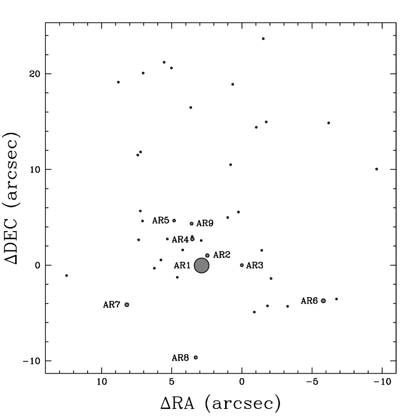
Figure 1: Location of the 42 wind-producing stars used in the simulations of the Arches cluster, relative to $\alpha(2000)$: $17^{h}\,45^{m}\,50.26^{s}$, $\delta(2000)$: $-28^{\circ}\,49^{\prime}\,22^{\prime\prime}.76$ (Figer et al., 2002). The radius of each circle corresponds (on a linear scale) to that star’s mass loss rate. Setting the scale is AR1, with $\dot{M}=1.7\times 10^{-4}\;M_{\odot}$ yr^-1.

In an attempt to represent both the identified stellar wind sources and the population of stars likely to be producing significant but currently undetected winds, we include 42 wind sources (listed in Table 1 and shown in Figure 1) in our simulations of the Arches cluster. The stars labeled AR1–AR9 correspond to the 9 radio sources identified by Lang (2002). The first 29 stars (labeled 1–29) in Table 1 have mass estimates greater than $60\;M_{\odot}$ (Figer et al., 2002), and are likely the most powerful sources of wind in the cluster. The remaining 13 stars used in the simulations have masses less than $60\;M_{\odot}$ but greater than $25\;M_{\odot}$ and are located on the north side of the cluster; they are included to better represent the spatial pattern of X-ray emission around the core of the cluster. Based on the broadening of the Br$\gamma$ line observed by Cotera et al. (1996), stars in the Arches cluster simulations are assigned wind velocities of $1,000$ km s^-1. The stars labeled AR1–AR9, which have observed 8.5 GHz flux densities, are assigned mass-loss rates according to Equation 1. Stars with no associated 8.5 GHz detection but with masses larger than $60\;M_{\odot}$ are assigned a mass-loss rate of $3\times 10^{-5}\;M_{\odot}$ yr^-1, which is equal to the lowest mass-loss rate inferred from the weakest observed 8.5 GHz signal from the Arches cluster (Lang, 2002). Stars with masses less than $60\;M_{\odot}$ are assigned a mass-loss rate of $3\times 10^{-6}\;M_{\odot}$ yr^-1; their winds will have little effect on the overall luminosity but may alter the shape of the X-ray-emitting region.

1.2 The Quintuplet Cluster

Slightly further north of Sgr A*, the Quintuplet cluster is located at $l=0.16^{\circ}$, $b=0.06^{\circ}$. The cluster has a total estimated mass of $\sim 10^{4}\;M_{\odot}$ and a mass density of $\sim 10^{3}\;M_{\odot}$ pc^-3 (Figer et al., 1999a). Like the objects in the Arches cluster, the known massive stars in the Quintuplet cluster have near-IR emission-line spectra indicating that they too have evolved away from the zero-age main sequence and now produce high-velocity stellar winds with terminal speeds of $500$–$1,000$ km s^-1.

Figer et al. (1999a) obtained K-band spectra of 37 massive stars in the Quintuplet cluster and found that 33 could be classified as WR stars, OB supergiants, or luminous blue variables (LBVs), implying a range of wind mass-loss rates $\dot{M}\sim(0.1$–$6.6)\times 10^{-5}\;M_{\odot}$ yr^-1. VLA continuum images at 6 cm and 3.6 cm of the Sickle and Pistol H ii regions reveal eight point sources located in the vicinity of the Quintuplet cluster, including the radio source at the position of the Pistol nebula (Lang et al., 1999). These are labeled QR1 through 7, and the Pistol star, in Figure 2 below.

The near-IR counterparts of QR4 and QR5 are hot, massive stars with high mass-loss rates, one an OB i supergiant and the other a WN9/Ofpe (Figer et al., 1999a). The sources QR1, QR2, and QR3 also have spectral indices consistent with stellar wind sources, but they have no obvious NICMOS stellar counterparts. Lang et al. (1999) speculated that this may be due to variable extinction associated with a dense molecular cloud located in front of the cluster. Given the uncertainty, and possible variation, in stellar identification for these 5 objects, we therefore adopt a value of $\sim 500$ km s^-1 (typical in OB supergiants) for the speed of their wind. The Pistol star, on the other hand, is a prominent source in the near-IR NICMOS image, and is evidently a luminous blue variable (Figer et al., 1998) possessing a powerful stellar wind, though with a terminal speed of only $v_{\infty}\sim 100$ km s^-1.

In our simulations of the Quintuplet cluster, we include 31 massive stars with spectral classifications identified by Figer et al. (1999a), using estimates for the wind parameters of each star according to its spectral type. Wind velocities are determined according to the broad spectral type of each star: we assume a velocity of $1,000$ km s^-1 for winds from WR stars, $500$ km s^-1 winds for OB supergiants, and $100$ km s^-1 for the Pistol star, a LBV.

For those stars that are radio sources (QR1–QR3, QR6, and QR7 from Lang et al., 1999), mass-loss rates are determined according to Equation 1. For the rest of the stars, we estimate the mass-loss based on the spectral classifications by Figer et al. (1999a). For OB stars, the mass-loss rate was assumed to be $10^{-5}\;M_{\odot}$ yr^-1 for stars with classification higher than BO. For smaller stars, the mass-loss rate was assumed to be $10^{-6}\;M_{\odot}$ yr^-1. For Wolf-Rayet stars, we use a luminosity-mediated mass-loss relation (Wellstein & Langer, 1999):

$$log\left(-\dot{M}_{\rm WR}\over M_{\odot}\;yr^{-1}\right)=k+1.5log\left(L\over L_{\odot}\right)-2.85X_{s},$$ (2)

where $L$ is the stellar luminosity from Figer et al. (1999a), $X_{s}$ is the hydrogen mass fraction, and $k$ is a constant which we calibrated using our radio-determined mass-loss rates. The locations and wind parameters of the stellar wind sources are summarized in Table 2, and their relative positions are shown in Figure 2.

2 The Physical Setup

Our calculations use the three-dimensional smoothed particle hydrodynamics (SPH) code discussed in Fryer & Warren (2002) and Warren et al. (2004), modified as described in Rockefeller et al. (2004) to include stellar wind sources. The gridless Lagrangean nature of SPH allows us to concentrate spatial resolution near shocks and model gas dynamics and wind-wind interactions on length scales that vary by several orders of magnitude within a single calculation.

We assume that the gas behaves as an ideal gas, according to a gamma-law ($\gamma=5/3$) equation of state. The effect of self-gravity on the dynamics of the gas should be negligible compared to the effect of the central cluster potential; we calculate gravitational effects by approximating the potential of each cluster with a Plummer model.

The computational domain for the simulation of each cluster is a cube approximately $6$ pc on a side, centered on the middle of the cluster. To simulate “flow-out” conditions, particles passing through the outer boundary are removed from the simulation. The initial conditions assume that the space around and within each cluster is empty; massive stars in each cluster then inject matter into the volume of solution via winds as the calculation progresses. The number of particles in each simulation initially grows rapidly, but reaches a steady number ($\sim 6.6$ million particles for simulations of the Arches cluster and $\sim 3.3$ million particles for the Quintuplet simulations, since there are fewer identified wind sources in the latter) when the addition of particles from wind sources is compensated by the loss of particles through the outer boundary of the computational domain.

2.1 Cluster Potential

We model the gravitational potential $\Phi$ of a cluster using a Plummer model (Plummer, 1911),

$$\Phi(r)=\frac{-GM}{\sqrt{r^{2}+b^{2}}}\;,$$ (3)

where $M$ is the total mass of the cluster. The radial density profile assumed for the cluster is therefore

$$\rho(r)=\rho_{0}{\left(1+\frac{r^{2}}{b^{2}}\right)}^{-5/2}\;,$$ (4)

where the central density $\rho_{0}$ is

$$\rho_{0}=\frac{3M}{4\pi b^{3}}\;.$$ (5)

We note that the spatial distributions of massive stars in the clusters are not entirely consistent with the distribution implied by the Plummer potential; for example, the average projected distance of both the set of massive stars and the set of all observed stars in the Arches cluster is roughly twice the average distance predicted by a Plummer model based on the estimated total mass and central density of the cluster. We include the Plummer potential to approximate the combined gravitational influence of the entire cluster, including the estimated mass of stars too small or dim to be observed.

Figer et al. (1999a) provide estimates of the total mass of each cluster by measuring the mass of observed stars, assuming a Salpeter IMF slope, and extrapolating down to $1\;M_{\odot}$—observed stars account for at most 25% of the mass of the Arches cluster and 16% of the mass of the Quintuplet cluster. They also estimate the density of each cluster by determining the volume of the cluster from the average projected distance of stars from the cluster center, and dividing the total mass by this volume; because the values are calculated using the total cluster mass but only the average projected cluster radius, the density estimates are probably closer to the central densities than the average densities. We assume that the values reported are the central densities of the clusters. The total cluster mass and central density and the calculated value of $b$ for each cluster are presented in Table 3.

2.2 Wind Sources

We implement wind sources as literal sources of SPH particles, using the scheme described in Rockefeller et al. (2004). The mass loss rates and wind velocities inferred from observations are reported in Tables 1 and 2. We position each source at its observed $x$ and $y$ location and choose the $z$ coordinate randomly, subject to the constraint that the wind sources are uniformly distributed over a range in $z$ equal to the observed range in $x$ and $y$. The choice of $z$ positions has a much smaller effect on the X-ray luminosity than the choice of mass-loss rate (discussed below); Rockefeller et al. (2004) performed simulations of wind sources in the central few parsecs of the Galaxy with two different sets of $z$ positions, and the average $2-10$ keV X-ray luminosity from the central 10^′′ of the simulations differed by only 16% ($7.50\times 10^{31}$ erg s^-1 arcsec^-2 from a simulation with a dense arrangement of wind sources in the center of the volume of solution versus $6.45\times 10^{31}$ erg s^-1 arcsec^-2 from a simulation with wind sources uniformly distributed in $z$). In addition, Raga et al. (2001) conducted three simulations of the Arches cluster in which $z$ positions of sources were chosen by sampling from a distribution function $f(R)\propto R^{-2}$; they found a difference in $0.5-8$ keV X-ray luminosity of only 3% between the most and least luminous simulations.

Figure 1 shows the positions in the sky plane of the wind sources in the Arches cluster, while Figure 2 shows the wind sources in the Quintuplet cluster; the size of the circle marking each source corresponds to the relative mass loss rate (on a linear scale) for that star. The initial temperature of the winds is not well known; for simplicity, we assume that all of the winds have a temperature of $10^{4}$ K. Our results are fairly insensitive to this value, however, since the temperature of the shocked gas is determined primarily by the kinetic energy flux carried into the collision by the winds. The sources are assumed to be stationary over the duration of the simulation.

We conduct two simulations of the wind-wind interactions in each cluster; the simulations differ only in the choice of mass-loss rate for each star, with the wind speed assumed constant. The “standard” simulations use mass-loss rates inferred from observations as described in §§ 1.1 and 1.2, while the “high-$\dot{M}$” simulations use mass-loss rates increased from the standard value by a factor 2.

3 Observations

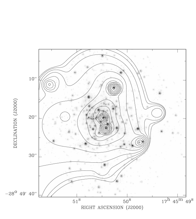
Figure 3: Chandra ACIS-I 1–9 keV intensity contours overlaid on a HST NICMOS image of the Arches cluster. The image is exposure-corrected and is adaptively smoothed with the CIAO csmooth routine ($S/N\sim 3\sigma$). The contour levels are at $(31,32,34,38,46,62,94,158,286,542,1054,2078,4126)\times 10^{-3}{\rm~{}counts~{}s^{-1}~{}arcmin^{-2}}$.

An on-axis Chandra observation of the Arches cluster was taken on 2004 June 8 for 98.6 ksec. The ACIS-I detector was placed at the focal plane. The data were analyzed with the latest CIAO (version 3.1). While results of this observation will be presented in an upcoming paper (Wang, 2004), we concentrate here on the comparison of the data with the simulations. Figure 3 shows an overlay of an X-ray intensity contour map on a HST NICMOS image of the Arches cluster (Figer et al., 1999b). The actual spatial resolution (with a FWHM $\lesssim 1^{\prime\prime}$) is better than what appears on this smoothed image. The position coincidence of the point-like X-ray sources and bright near-IR objects is apparent. To compare with the simulated cluster wind properties, we remove a region of twice the 90% energy-encircled radius around each of the sources.

4 Results

All four simulations were run significantly past the point in time when the stellar winds fill the volume of solution and gas shocked in wind-wind collisions fills the core of each cluster. The Arches cluster simulations were run past $t=10,000$ yr; the Quintuplet simulations were run for over $14,000$ yr. The winds in each simulation reach the edge of the volume of solution after $\sim 3,000$ yr, but the most relevant timescale for determining when the simulations reach a steady level of X-ray luminosity is the time required to fill the core of each cluster with shocked gas. The Arches cluster core is roughly five times smaller in radius than the core of the Quintuplet cluster, so the X-ray luminosity from the Arches simulations reaches a steady value relatively quickly compared to the Quintuplet simulations.

4.1 Total Flux and Time Variation

In order to calculate the observed continuum spectrum, we assume that the observer is positioned along the positive $z$-axis at infinity and we sum the emission from all of the gas injected by the stellar wind sources into the volume of each calculation. For the conditions encountered in the two clusters, scattering is negligible and the optical depth is always less than unity. For these temperatures and densities, the dominant components of the continuum emissivity are electron-ion ($\epsilon_{ei}$) and electron-electron ($\epsilon_{ee}$) bremsstrahlung. We assume that the gas is in ionization equilibrium, although spectra obtained from the Arches cluster with Chandra indicate the presence of line emission at $6.4$ keV; however, no other significant lines are observed, so our use of a bremsstrahlung model without line emission is a reasonable approximation. Future, more refined versions of the calculations reported here will need to include the effects of partial ionization in the shocked gas, a condition suggested by the iron line emission. We note, however, that the overall energetics and diffuse X-ray luminosity calculated by assuming full ionization err only marginally since the fraction of charges free to radiate via bremsstrahlung should be very close to one.

The X-ray luminosities calculated from our simulations support the recent result of Law & Yusef-Zadeh (2004) that the majority of the X-ray emission from these clusters (e.g., $\sim 60\%$ for Arches) is probably due to point sources. The diffuse 0.2–10 keV X-ray luminosity calculated from our “standard” Arches cluster simulation—$5.4\times 10^{34}$ erg s^-1—falls below the 0.2–10 keV luminosity of $4.1\times 10^{35}$ erg s^-1 from the A1 and A2 components reported in Yusef-Zadeh et al. (2002); the simulation using elevated estimates for the mass-loss rates produces $2.2\times 10^{35}$ erg s^-1 between 0.2 and 10 keV, or 53% of the emission observed by Chandra. On the other hand, Law & Yusef-Zadeh (2004) now identify A1 and A2 as point-like components; after subtracting the contributions of A1 and A2, Yusef-Zadeh et al. (2002) find that the A3 component has a 0.5–10 keV luminosity of $\sim 1.6\times 10^{34}$ erg s^-1. Our “standard” simulation produces $2.7\times 10^{34}$ erg s^-1 between 0.5 and 10 keV; lowering the mass-loss estimates of all wind sources by $\sim 30\%$ or slightly decreasing the assumed wind velocities would produce even better agreement.

Our “standard” and “high-$\dot{M}$” simulations of the Quintuplet cluster produce $1.5\times 10^{33}$ erg s^-1 and $5.9\times 10^{33}$ erg s^-1, respectively, between 0.5 and 8 keV. Law & Yusef-Zadeh (2004) estimate a 0.5–8 keV luminosity of $\sim 1\times 10^{34}$ erg s^-1 for the diffuse emission from the Quintuplet cluster, but they point out that other regions of diffuse emission to the north and south of the cluster introduce a complicated pattern of background emission and limit the precision of this estimate.

The long-term variation of the X-ray luminosity as a function of time demonstrates some of the key differences between the two clusters. Figures 4 and 5 show the time variation of the 0.5–8 keV X-ray luminosity from all four simulated clusters. Each large graph shows the variation over the course of the entire simulation ($>10,000$ yr for the simulations of the Arches cluster, and $>14,000$ yr for the Quintuplet simulations), while each inset graph shows variation over $1,000$ timesteps, or $\sim 150$ yr. The fact that the Quintuplet cluster is nearly five times larger in radius than the Arches cluster means that much more time is required for shocked gas to fill the central region. The Arches cluster reaches a steady X-ray luminosity after less than $2,000$ yr, while the luminosity of the Quintuplet cluster does not clearly level off until more than $10,000$ yr have passed.

The two clusters also exhibit differences in the size of short-term fluctuations in X-ray luminosity. Both simulations of the Arches cluster show short-term variations in luminosity of $\sim 1\%$ over timescales of $\sim 50$ yr, while the X-ray luminosity in the “standard” Quintuplet simulation fluctuates by $\sim 4\%$, and short-term variations in the “high-$\dot{M}$” simulation of the Quintuplet cluster are as large as $\sim 7\%$.

4.2 Spatial Variation of the X-ray Flux

Figure 3 shows that many of the bright X-ray peaks in the Arches cluster correspond to actual stars, presumably binaries whose binary wind interactions produce the strong localized X-ray emission. These sources must be subtracted to study the diffuse X-ray emission.

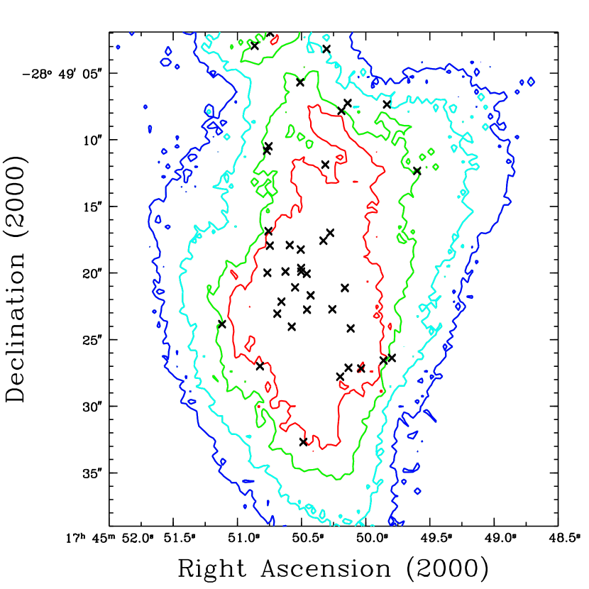
Figure 6: Contours of column-integrated 0.5–8 keV X-ray luminosity per arcsec² from the “standard” (left) and “high-$\dot{M}$” simulations of the Arches cluster. In order from blue to cyan to green to red, the luminosities indicated by the contours are $10^{30}$, $2.5\times 10^{30}$, $8\times 10^{30}$, and $2\times 10^{31}$ ergs s^-1 arcsec^-2. The crosses indicate the positions of wind sources included in the simulations.

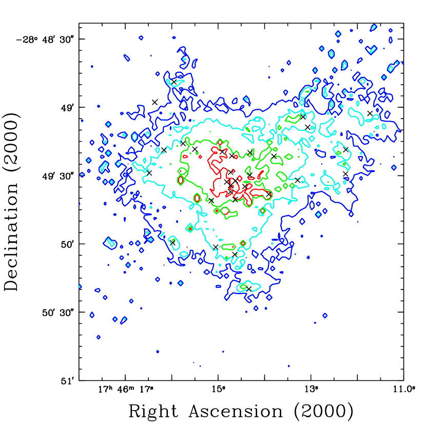
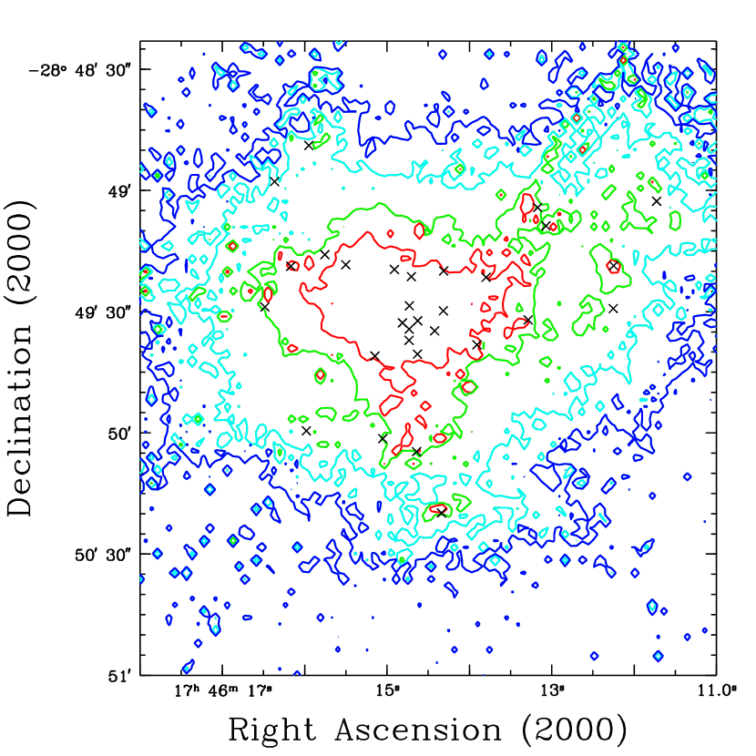
Figure 7: Contours of column-integrated 0.5–8 keV X-ray luminosity per arcsec² from the “standard” (left) and “high-$\dot{M}$” simulations of the Quintuplet cluster. In order from blue to cyan to green to red, the luminosities indicated by the contours are $7\times 10^{28}$, $1.8\times 10^{29}$, $7\times 10^{29}$, and $2\times 10^{30}$ ergs s^-1 arcsec^-2. The crosses indicate the positions of wind sources included in the simulations.

The simulated 0.5–8 keV X-ray contours from the region near the core of the Arches cluster, shown in Figure 6, are generally comparable to the contours generated from Chandra observations (Figure 3; see also Figure 2b, Yusef-Zadeh et al., 2002). The strongest emission in the simulations and in Chandra images comes from the core of the cluster, and both sets of contours form elliptical patterns aligned primarily north-south. X-ray contours from the simulation of the Quintuplet cluster are shown in Figure 7; the Quintuplet cluster is significantly less dense than the Arches cluster, so the X-ray emission is correspondingly less strongly peaked toward the center of the cluster.

The plots in Figure 8 show the total 0.5–8 keV luminosity from concentric columns aligned along the line of sight and extending outward in radius from the center of the Arches (left) and Quintuplet (right) clusters. The most luminous gas in the Arches cluster is confined to within $20^{\prime\prime}$ of the center of the cluster; in contrast, we include stars beyond $50^{\prime\prime}$ in the Quintuplet cluster, and its luminosity continues to increase even beyond a radius of $50^{\prime\prime}$.

Similarly, the plots in Figure 9 show the 2–8 keV X-ray flux per square arcmin as a function of distance from the center of each cluster from all four simulations. The individual crosses and error bars in the graph from the Arches cluster represent flux measurements from Chandra observations of the cluster, after point sources have been removed and an estimate of the background X-ray flux has been subtracted. Here we assume that all of the emission centered around NICMOS stellar sources is due to binary wind interactions. The estimated background—0.064 counts s^-1 arcmin^-2—is the average number of counts obtained in an annulus between radii of $0.5^{\prime}$ and $0.9^{\prime}$. The simulations of the Arches cluster apparently produce more X-rays near the center of the cluster but decrease in intensity more rapidly toward larger radii. The relatively flat surface brightness profile evident in the Chandra data outside a radius of $0.3^{\prime}$ may arise in part from the presence of additional background X-ray emission near the Galactic center. It may also indicate confinement of the X-ray-emitting gas in the Arches cluster by ram pressure exerted by a molecular cloud or other external medium surrounding the cluster; our calculations include no such medium, so the simulated gas escapes and cools more rapidly as it leaves the core of the cluster.

One way to constrain the amount of confining material surrounding the cluster is to measure expansion velocities of the gas out of the cluster. In our simulations, which did not include confining gas, the material accelerates until it reaches an asymptotic velocity limit roughly equal to the mean wind velocity (Figure 10). In the Arches cluster, we reach that limit. In the (larger) Quintuplet cluster, that limit apparently occurs at a distance from the cluster center that is larger than the size of the simulation. However, if molecular clouds or additional stars with strong winds are producing a confining ram pressure around this cluster, the outflowing gas will decelerate. Measurements of this velocity will constrain the parameters of the surrounding material; future simulations can use these constraints to include the effects of this material.

5 Discussion

Although the diffuse X-ray flux in clusters may be used to probe stellar mass-loss, two notable complications in the case of the Arches and Quintuplet clusters are the X-ray background present in the Galactic center, and the contributions made to the overall emission by point (i.e., binary wind) sources. The contribution made by the X-ray background is difficult to quantify; Law & Yusef-Zadeh (2004) report that background contributions lead to significant uncertainty in the measured X-ray flux from the Quintuplet cluster. The contribution from point sources is easier to handle; with its relatively high spatial resolution, Chandra can produce reasonable images in which the required point-source subtraction may be made. Point sources in the Arches cluster all exhibit a 6.7 keV line; the absence of such a line in the spectrum of the diffuse emission indicates that the point-source contribution to the diffuse emission is not likely to be significant.

If, based on the observations made by Yusef-Zadeh et al. (2002), we assume that A1 and A2 are not point-like and do not subtract the contributions of point sources from the overall X-ray flux, it appears that the diffuse X-ray flux is consistent with higher mass-loss rates than the ($0.3\times 10^{-5}\;M_{\odot}$ yr^-1) $3\times 10^{-5}\;M_{\odot}$ yr^-1 assumed for stars (less than) above 60 M_⊙. As we have seen, however, the observed point-source-subtracted diffuse emission matches our calculated X-ray flux to within a factor 2 when we adopt the currently accepted stellar mass-loss rates. Indeed, lowering the mass-loss rate estimates of all wind sources by about $30\%$ would produce significant agreement between theory and observation. But we must make sure that we have a complete accounting of all the wind sources and carry through with a more careful point-source subtraction before we can completely confirm such claims.

The fact that the simulated X-ray flux density from the Arches cluster drops off more rapidly than the observed profile (see Figure 9) means that (1) we may have underestimated the contribution of the X-ray background; or, (2) we have ignored the possibly important dynamical influence of a confining molecular gas outside the cluster. Interpreting data beyond these radii (roughly $0.3^{\prime}$ for Arches and $1.0^{\prime}$ for Quintuplet) requires more detailed information on the cluster environment there.

X-rays do prove to be an ideal probe of bulk mass-loss rates in clusters. The X-ray emission depends sensitively on the mass-loss rates of the constituent stars and, based on our simulations of the Arches cluster, we can already limit the mass-loss rates to within a factor of 2 of the currently accepted values. This also implies that the assumed abundances in the Galactic center environment are essentially correct, since the mass-loss rates from stellar models depend on the adopted metallicity. In addition, studying the X-ray emission from the outer region of the cluster may eventually lead to a better understanding of the medium within which the cluster is embedded. This is clearly relevant to the question of how these unusual clusters came to be, and the relative roles played by “standard star formation” versus stellar capture from outside the cluster. The inferred stellar constituents of these clusters (Cotera et al., 1996; Figer et al., 1999a, e.g.,) also seem to be consistent with the required mass loss rates, so the inferred unusual mass function of the Arches, Quintuplet, and Central clusters continues to pose a challenge to our understanding of how these stellar aggregates were first assembled.

Acknowledgments This research was partially supported by NASA grant NAG5-9205 and NSF grant AST-0402502 at the University of Arizona, and has made use of NASA’s Astrophysics Data System Abstract Service. FM is grateful to the University of Melbourne for its support (through a Sir Thomas Lyle Fellowship and a Miegunyah Fellowship). This work was also funded under the auspices of the U.S. Dept. of Energy, and supported by its contract W-7405-ENG-36 to Los Alamos National Laboratory and by a DOE SciDAC grant number DE-FC02-01ER41176. The simulations were conducted primarily on the Space Simulator at Los Alamos National Laboratory. This research used resources of the National Energy Research Scientific Computing Center, which is supported by the Office of Science of the U.S. Department of Energy under Contract No. DE-AC03-76SF00098.

Table 1: Parameters for the Arches Cluster Wind Sources

Star	x	y	z	v	$\dot{M}$
	(arcsec)	(arcsec)	(arcsec)	(km s-1)	(${10}^{-5}\;M_{\odot}$ yr-1)
1, 0AR3	0+0.00	0+0.00	0+8.38	1,000	03.2
2	0$-$6.75	0$-$3.53	+10.70	1,000	03.0
3, 0AR7	0+8.20	0$-$4.13	0+2.66	1,000	04.2
4, 0AR5	0+4.83	0+4.66	0+2.71	1,000	03.0
5, 0AR8	0+3.29	0$-$9.64	0$-$5.31	1,000	03.6
6, 0AR1	0+2.87	0$-$0.03	0$-$1.85	1,000	17.0
7, 0AR4	0+3.53	0+2.73	0$-$5.72	1,000	03.9
8, 0AR2	0+2.46	0+1.01	0+2.78	1,000	03.9
9	0+0.80	+10.50	0+0.23	1,000	03.0
10	0$-$1.83	0$-$4.25	0$-$0.90	1,000	03.0
11	0$-$1.03	+14.41	0+6.83	1,000	03.0
12	0+1.01	0+4.98	$-$11.46	1,000	03.0
13	0$-$2.08	0$-$1.39	0+6.12	1,000	03.0
14	0+6.24	0$-$0.32	0+5.15	1,000	03.0
15	0+7.24	0+5.67	$-$14.94	1,000	03.0
16	0+4.22	0+1.59	$-$14.62	1,000	03.0
17	0$-$0.89	0$-$4.90	+14.59	1,000	03.0
18, AR9	0+3.58	0+4.34	+13.79	1,000	03.2
19, AR6	0$-$5.81	0$-$3.72	0$-$4.97	1,000	04.5
20	0+2.90	0+2.58	0$-$3.20	1,000	03.0
21	0+7.36	0+2.65	+10.49	1,000	03.0
22	0+0.24	0+5.55	0$-$8.01	1,000	03.0
23	+12.50	0$-$1.08	+14.43	1,000	03.0
24	0$-$1.42	0+1.55	0+9.62	1,000	03.0
25	0$-$3.26	0$-$4.30	0$-$8.37	1,000	03.0
26	0+4.60	0$-$1.27	+13.43	1,000	03.0
27	0+5.31	0+2.74	0+4.80	1,000	03.0
28	0+5.77	0+0.55	+10.79	1,000	03.0
29	0+7.08	0+4.62	+11.95	1,000	03.0
36	0$-$6.19	+14.87	0$-$8.33	1,000	03.0
37	0+3.54	0+2.99	0+5.89	1,000	03.0
49	0$-$1.74	+14.97	0+9.01	1,000	00.3
61	0$-$1.53	+23.67	0+2.02	1,000	00.3
75	0+7.42	+11.51	0+4.86	1,000	00.3
108	0+7.22	+11.83	0+7.08	1,000	00.3
111	0+0.65	+18.90	$-$12.39	1,000	00.3
116	0+3.64	+16.48	+12.31	1,000	00.3
126	0+8.80	+19.13	0$-$0.92	1,000	00.3
129	0$-$9.61	+10.04	0+2.44	1,000	00.3
132	0+7.04	+20.08	0+6.02	1,000	00.3
149	0+5.54	+21.20	0$-$5.47	1,000	00.3
156	0+5.02	+20.61	0+7.93	1,000	00.3

Table 2: Parameters for the Quintuplet Cluster Wind Sources

Star	x	y	z	v	$\dot{M}$
	(arcsec)	(arcsec)	(arcsec)	(km s-1)	(${10}^{-5}\;M_{\odot}$ yr-1)
QR1	0$-$3.30	+20.10	$-$36.41	0string500	08.00
QR2	0$-$0.30	+21.80	0+9.39	0string500	15.10
QR3	0+8.30	+22.90	$-$42.78	0string500	06.70
QR6	0$-$1.80	0+9.00	+31.80	1,000	06.10
QR7	0+3.00	0+1.00	$-$26.99	1,000	13.00
76	0$-$9.00	$-$36.60	0$-$9.50	1,000	00.28
134, Pistol	0$-$4.50	$-$21.90	$-$28.26	0string100	03.80
151	0+1.50	$-$18.80	$-$20.94	1,000	01.10
157	+15.00	$-$17.00	0+8.82	0string500	00.16
235	0$-$4.50	0+1.50	0$-$2.91	1,000	03.70
240	$-$15.00	0+3.80	0$-$9.06	1,000	03.30
241, QR5	0$-$3.00	0+4.80	+39.75	1,000	06.60
250	0$-$7.50	0+7.10	+48.44	0string500	01.00
256	$-$24.00	0+9.80	0$-$9.66	1,000	00.70
257	0$-$4.50	0+9.50	$-$19.34	0string500	01.00
269	0$-$9.00	+11.90	+24.33	0string500	00.10
270, QR4	0$-$3.00	+13.10	$-$29.77	0string500	01.40
274	$-$39.00	+12.60	+42.80	1,000	00.67
276	+22.50	+12.70	0$-$7.87	0string500	00.10
278	0$-$3.00	0+7.50	$-$36.93	0string500	01.00
301	$-$16.50	+20.00	0$-$4.93	0string500	00.10
307	0$-$9.00	+21.50	$-$41.15	0string500	01.00
309	$-$39.00	+22.90	$-$38.32	1,000	00.26
311	+18.00	+22.50	+34.69	0string500	00.10
320	+12.00	+25.30	$-$18.66	1,000	00.61
344	$-$27.00	+32.40	0+4.04	0string500	00.10
353	+55.50	+36.70	0$-$6.15	1,000	00.22
358	$-$25.50	+36.80	$-$15.30	0string500	00.32
362	$-$46.50	+38.40	$-$13.75	0string100	03.00
381	+21.00	+42.80	$-$22.20	0string500	00.40
406	+15.00	+51.50	$-$26.93	0string500	00.10

Table 3: Properties of the Arches and Quintuplet Clusters

Cluster	M	$\rho_{0}$	b
	($M_{\odot}$)	($M_{\odot}$ pc-3)	(pc)
Arches	$2.0\times 10^{4}$	$6.3\times 10^{5}$	0.20
Quintuplet	$6.3\times 10^{3}$	$1.6\times 10^{3}$	0.98

Figure 4: The 0.5–8 keV X-ray luminosity versus time from the “standard” (left) and “high-$\dot{M}$” simulations of the Arches cluster. The large plot shows the variation in luminosity over the entire calculation, while the inset plot shows variation on a timescale of $\sim$ 10 years. The winds fill the core of the cluster after $\sim$ 2,000 years.

Figure 5: The 0.5–8 keV X-ray luminosity versus time from the “standard” (left) and “high-$\dot{M}$” simulations of the Quintuplet cluster. The large plot shows the variation in luminosity over the entire calculation, while the inset plot shows variation on a timescale of $\sim$ 10 years. The winds fill the core of the cluster after $\sim$ 10,000 years.

Figure 8: Total 0.5–8 keV X-ray luminosity from concentric cylinders aligned with the center of the Arches (left) and Quintuplet clusters. The lower line in each graph represents the “standard” simulation of that cluster; the upper line represents the “high-$\dot{M}$” simulation.

Figure 9: The 2–8 keV X-ray flux per arcmin² from concentric cylinders aligned with the center of the Arches (left) and Quintuplet clusters. The lower line in each graph represents the “standard” simulation of that cluster; the upper line represents the “high-$\dot{M}$” simulation. Crosses and error bars in the left graph represent flux measurements from Chandra observations of the Arches cluster.

Figure 10: Average radial velocity of gas in the “standard” simulations of the Arches (left) and Quintuplet clusters, versus distance from the center of each cluster.

References

- Cantó et al. (2000) Cantó, J., Raga, A. C., & Rodríguez, L. F. 2000, ApJ, 536, 896.
- Cotera et al. (1996) Cotera, A. S., Erickson, E. F., Colgan, S. W. J., Simpson, J. P., Allen, D. A., & Burton, M. G. 1996, ApJ, 461, 750.
- Figer et al. (1998) Figer, D. F., Najarro, F., Morris, M., McLean, I. S., Geballe, T. R., Ghez, A. M., & Langer, N. 1998, ApJ, 506, 384.
- Figer et al. (1999a) Figer, D. F., McLean, I. S., & Morris, M. 1999a, ApJ, 514, 202.
- Figer et al. (1999b) Figer, D. F., Kim, S. S., Morris, M., Serabyn, E., Rich, R. M., & McLean, I. S. 1999b, ApJ, 525, 750.
- Figer et al. (2002) Figer, D. F., Najarro, F., Gilmore, D., Morris, M., Kim, S. S., Serabyn, E., McLean, I. S., Gilbert, A. M., Graham, J. R., Larkin, J. E., Levenson, N. A. & Teplitz, H. I. 2002, ApJ, 581, 258.
- Fryer & Warren (2002) Fryer, C. L. & Warren, M. S. 2002, ApJ, 574, L65.
- Gerhard (2001) Gerhard, O. 2001, ApJ, 546, L39.
- Lang et al. (1999) Lang, C. C., Figer, D. F., Goss, W. M., & Morris, M. 1999, AJ, 118, 2327.
- Lang et al. (2001) Lang, C. C., Goss, W. M., & Rodríquez, L. F. 2001, ApJ, 551, L143.
- Lang (2002) Lang, C. C. 2002, in A Massive Star Odyssey, from Main Sequence to Supernova, IAU Symp. 212, Eds. K. A. van der Hucht, A. Herrero, & C. Esteban.
- Law & Yusef-Zadeh (2004) Law, C. & Yusef-Zadeh, F. 2004, ApJ, accepted.
- McMillan & Portegies Zwart (2003) McMillan, S. L. W. & Portegies Zwart, S. F. 2003, ApJ, 596, 314.
- Melia & Falcke (2001) Melia, F. & Falcke, H. 2001, ARA&A, 39, 309.
- Morris (1993) Morris, M. 1993, ApJ, 408, 496.
- Nagata et al. (1995) Nagata, T., Woodward, C. E., Shure, M., & Kobayashi, N. 1995, AJ, 109, 1676.
- Ozernoy et al. (1997) Ozernoy, L. M., Genzel, R., and Usov, V. V. 1997, MNRAS, 288, 237.
- Panagia & Felli (1975) Panagia, N. & Felli, M. 1975, A&A, 39, 1.
- Plummer (1911) Plummer, H. C. 1911, MNRAS, 71, 460.
- Raga et al. (2000) Raga, A. C., Navarro-González, R., & Villagrán-Muniz, M. 2000, Rev. Mexicana Astron. Astrofis., 36, 67.
- Raga et al. (2001) Raga, A. C., Velázquez, P. F., Cantó, J., Masciadri, E., & Rodríguez, L. F. 2001, ApJ, 559, L33.
- Rockefeller et al. (2004) Rockefeller, G., Fryer, C. L., Melia, F., & Warren, M. S. 2004, ApJ, 604, 662.
- Serabyn et al. (1998) Serabyn, E., Shupe, D., & Figer, D. F. 1998, Nature, 394, 448.
- Wang (2003) Wang, Q. D. 2003, IAU Symposium No. 214: High Energy Processes and Phenomena in Astrophysics, Eds: X.D. Li, V. Trimble, & Z.R. Wang. 214, 32
- Wang (2004) Wang, Q. D. 2004, in preparation.
- Warren et al. (2004) Warren, M. S., Rockefeller, G., & Fryer, C. L. 2004, in preparation.
- Wellstein & Langer (1999) Wellstein, S. & Langer, N. 1999, A&A, 350, 148
- Yusef-Zadeh et al. (2002) Yusef-Zadeh, F., Law, C., Wardle, M., Wang, Q. D., Fruscione, A., Lang, C. C., & Cotera, A. 2002, ApJ, 570, 665.