A NLTE line blanketed model of a solar type star

Abstract

We present LTE and NLTE atmospheric models of a star with solar parameters, and study the effect of treating many thousands of Iron group lines out of LTE on the computed atmospheric structure, overall absolute flux distribution, and the moderately high resolution spectrum in the visible and near UV bands. Our NLTE modeling includes the first two or three ionization stages of 20 chemical elements, up to and including much of the Fe -group, and includes about 20000 Fe I and  II lines. We investigate separately the effects of treating the light metals and the Fe -group elements in NLTE. Our main conclusions are that 1) NLTE line blanketed models with direct multi-level NLTE for many actual transitions gives qualitatively similar results as the more approximate treatment of Anderson (1989) for both the Fe  statistical equilibrium and the atmospheric $T_{\rm kin}$ structure, 2) models with many Fe  lines in NLTE have a $T_{\rm kin}$ structure that agrees more closely with LTE semi-empirical models based on center-to-limb variation and a wide variety of spectra lines, whereas LTE models agree more with semi-empirical models based only on an LTE calculation of the Fe I excitation equilibrium, 3) the NLTE effects of Fe -group elements on the model structure and $F_{\lambda}$ distribution are much more important than the NLTE effects of all the light metals combined, and serve to substantially increases the violet and near UV $F_{\lambda}$ level as a result of NLTE Fe over-ionization. These results suggest that there may still be important UV opacity missing from the models. However, the choice of the species and multiplet dependent van der Waals broadening enhancement also plays a significant role in determining whether LTE or NLTE models provide a close fit to the near UV flux level. We also find that the RMS deviation of the shape of the rectified high resolution synthetic spectrum from that of the the observed spectrum is not significantly affected by the inclusion of NLTE effects.

1 Introduction

Of the many fronts on which models of stellar atmospheres and spectrum formation need to be made more realistic, one is the treatment of the thermodynamic state of the gas and the radiation field. A particular difficulty in this regard is that complex atoms and ions such as those of Fe  and the Fe -group elements have a particularly rich term structure with many transitions that need to be accounted for in a realistic equilibrium solution. The very thing that makes these species problematic also gives impetus to their accurate treatment: their many transitions provide a dense line opacity that veils the spectrum and partially controls the value of the broad-band emergent flux, especially in the violet and UV bands of late-type stars. We emphasize at the outset that the accuracy of atmospheric models depends on both the physical realism of the modeling, and on the quality and completeness of the input physical data. The inadequacies of the latter are documented in, for example, Kurucz (2002). Here we study the effect of improvement in the former while holding the latter fixed. The goal of this paper is to ask and answer this question: what are the effects on the model of a late-type star and its computed spectrum of treating the equilibrium state of the Fe -group elements and many of their transitions more realistically than has been done in the past, while holding fixed the other degrees of realism that typify current models of late-type stars. We have partially addressed this question for the Fe  equilibrium in red giant stars ((Short & Hauschildt, 2003)). Here we address the question more completely for Fe  and other Fe -group elements in a late-type main sequence (MS) star, namely one that has the parameters of the Sun.

Determination of the Fe abundance in the closest late-type star, the Sun, has been particularly problematic (see Kostik et al. (1996) for a very thorough discussion). Related to this has been the problem of correctly modeling the overall flux level in the near UV band (3000 to 4000Å) (Kurucz, 1992a), which is veiled by thousands of weak Fe I lines. The most widely used theoretical atmospheric models for late-type stars are the ATLAS series of models (Kurucz, 1994a) and the MARCS (most recently NMARCS) series of models (Plez et al., 1992), both of which make use of the simplifying assumption of Local Thermodynamic Equilibrium (LTE). As a result of the vast expansion of the input line lists in the early 1990’s, these theoretical LTE models have been more successful at fitting the solar flux distribution in the near UV band than have semi-empirical models such as that of Holweger & Mueller (Holweger & Mueller, 1974) (see, for example, Blackwell et al. (1995)). However, the details of line formation not only affect the predicted flux level directly by way of its effect on opacity, but also indirectly by way of the effect of opacity on the radiative equilibrium structure of the atmosphere. In the case of the Fe I spectrum and the UV flux level, it has been found that the approximation of LTE “conspires” to off-set errors in the atmospheric structure, and thus provide a deceptively accurate prediction of the UV flux level (see, for example, Kostik et al. (1996) and references therein for a thorough discussion). Anderson (1989) calculated theoretical NLTE models of the solar atmosphere with many opacity sources treated in NLTE and found that NLTE departures in the Fe equilibrium significantly affect the atmospheric T structure. The latter work is a significant development, however, it treats the NLTE radiative transfer problem is a more approximate way ((the multifrequency/multigray algorithm) rather than the more direct way employed here.

The atmospheres of late-type MS stars are translucent over large enough path lengths that non-locally determined radiative rates often dominate collisional rates for many transitions, causing departures from local thermodynamic equilibrium (LTE). Previous NLTE investigations of Fe I with atomic models of more limited scope than that used here (see Shchukina & Trujillo Bueno (2001) for a recent example) have found that the the weak Fe I lines become significantly weaker due to NLTE over-ionization. Therefore, both the atmospheric structure and the emergent spectrum should be calculated in the more general statistical equilibrium (SE), in which a set of coupled equations is solved for the rate at which every energy level of every ionization stage of every species is populated and de-populated by various collisional and radiative processes.

As a result of computational constraints, previous investigations of NLTE effects in the atmospheres of the Sun and other late-type stars have treated at most a few hundred spectral lines in SE while treating most of the strongest lines and most of the “haze” of weaker lines as LTE “background” opacity. The notable exception is the modeling of Anderson (1989) described above. However, for complex species such as Fe I and  II the method of Anderson (1989) solves the SE equations for model states composed of many real states (the multifrequency/multigray algorithm) rather than for real states. Recently, Short et al. (1999) have modified the multi-purpose atmospheric modeling and spectrum synthesis code, PHOENIX (Hauschildt & Baron, 1999), to greatly increase the number of chemical species that are treated in NLTE SE. As a result, over 100 000 spectral lines throughout the spectrum, including all of the strongest lines and many of the weaker lines that blanket the UV band, are now treatable in self-consistent NLTE. This includes $\sim$6900 lines of Fe I, $\sim$13600 lines of Fe II, and $\sim$35000 lines due to the first two ionization stages of the Fe -group elements Ti, Mn, Co, and Ni. Even this is a small fraction of the millions of spectral lines that collectively control the emergent flux, but it is a significant step forward in improving the realism of the models. The purpose of this study is to calculate theoretical models and synthetic spectra for the Sun, considered as a star, with the newly expanded NLTE treatment to assess the affect that large scale NLTE line blanketing has on the theoretical model structure and the synthetic spectrum in the problematic violet and near UV bands. In Section 2 we describe the computational modeling; in Section 3 we present our results, and we re-iterate our main conclusions in Section 4.

2 Modeling

PHOENIX makes use of a fast and accurate Operator Splitting/Accelerated Lambda Iteration (OS/ALI) scheme to solve self-consistently the radiative transfer equation and the NLTE statistical equilibrium (SE) rate equations for many species and overlapping transitions (Hauschildt & Baron, 1999). Recently Short et al. (1999) have greatly increased the number of species and ionization stages treated in SE by PHOENIX so that at least the lowest two stages of 24 elements, including the lowest six ionization stages of the 20 most important elements, including Fe and four other Fe -group elements, are now treated in NLTE. Short et al. (1999) contains details of the sources of atomic data and the formulae for various atomic processes. Table 1 shows which species have been treated in NLTE in the modeling presented here, and how many $E$ levels and $b-b$ (bound-bound) transitions are included in SE for each species. For the species treated in NLTE, only levels connected by transitions of $\log gf$ value greater than -3 (designated primary transitions) are included directly in the SE rate equations. All other transitions of that species (designated secondary transitions) are calculated with occupation numbers set equal to the Boltzmann distribution value with excitation temperature equal to the local kinetic temperature, multiplied by the ground state NLTE departure co-efficient for the next higher ionization stage. We have only included in the NLTE treatment those ionization stages that are non-negligibly populated at some depth in the Sun’s atmosphere. As a result, we only include the first one or two ionization stages for most elements.

NLTE effects can depend sensitively on the adopted values of atomic parameters that affect the rate of collisional and radiative processes. Atomic data for the energy levels and b-b transitions have been taken from Kurucz (1994b) and Kurucz & Bell (1995). We have used the resonance-averaged Opacity Project (Seaton et al., 1994) data of Bautista, et al. (1998) for the ground-state photo-ionization cross sections of Li I- II, C I- IV, N I- VI, O I- VI, Ne I, Na I- VI, Al I- VI, Si I- VI, S I- VI, Ca I- VII, and Fe I- VI. For the ground states of all stages of P and Ti and for the excited states of all species, we have used the cross sectional data previously incorporated into PHOENIX, which are from Reilman & Manson (1979) or those compiled by Mathisen (1984). We account for coupling among all bound levels by electronic collisions using cross sections calculated with the formula of Allen (1973). We do not use the formula of Van Regemorter (1962) for pairs of levels that are connected by a permitted radiative transition because we have found that doing so leads to rates for transitions within one species that are very discrepant with each other, and this leads to spurious results. The cross sections of ionizing collisions with electrons are calculated with the formula of Drawin (1961). We describe in this paper a perturbation analysis of collisional rates.

Table 2 shows the three levels of realism with which we model the equilibrium state of the gas and the radiation field. Unless otherwise noted, the realism of a synthetic spectrum calculation is always consistent with that of the input model used. Our NLTE modeling includes two levels of realism: 1) NLTE treatment for H, He, and important light metals up to, but not including, the Fe -group elements (designated NLTE_Light models), and 2) the same as the NLTE_Light models except that the Fe -group elements Ti, Mn, Fe Co, and Ni are also included in the NLTE treatment (designated NLTE_Fe models). The Fe -group elements play a special role in the atmospheres and spectra of late-type stars (Thevenin & Idiart, 1999); because of their spectacularly rich term structure a neutral or low ionization stage Fe -group element contributes between one and two orders of magnitude more lines to the spectrum than the corresponding stage of any lighter element. Finally, we note that all of the models in Table 2 also include many tens of millions additional lines from many atoms, ions and diatomic molecules in the approximation of LTE. Note that H^-, which is an important source of continuous opacity in late-type MS stars, is treated in LTE here.

2.1 Modeling limitations

Atomic parameters:

We do not make any attempt here to fine-tune the atomic parameters that control the formation of individual spectral lines. Such fine tuning of oscillator strengths ($gf$ values) and damping constants ($\gamma$ values) is necessary for the derivation of accurate abundances of particular species from the fit to particular spectral lines. Our purpose is to investigate the collective consequence of including NLTE effects in the formation of many spectral lines. We presume that errors in the atomic data in the line list of Kurucz (1992a) are random and will not bias the apparent collective effect of massive-scale NLTE.

Model structure:

We note that late-type stars generally have a chromospheric temperature inversion in their outer atmosphere. Because our models are in radiative/convective equilibrium, they have monotonically decreasing $T_{\rm kin}(\tau)$ structures. Therefore, the cores of strong lines that are sufficiently opaque to remain optically thick very high in the atmosphere, and for which the emergent radiation field is dominated by local thermal conditions where the line forms, will not be accurately reproducible with our model. We expect to predict too little flux in the cores of such lines. Also, as $\lambda$ decreases the atmosphere becomes increasingly opaque such that, in the case of the Sun, the entire pseudo-continuum at $\lambda<2500$Å  forms above the depth of minimum temperature ($T_{\rm min}$). Therefore, we must expect that theoretical atmospheric models will necessarily increasingly under-predict the emergent flux there, and we restrict our spectral fitting to $\lambda>3000$Å. For late-type stars with particularly active chromospheres, chromospheric pseudo-continuum emission may contaminate the flux at $\lambda$ values longer than $3000$Å, so caution must be used when comparing theoretical and observed flux.

Homogeneity:

Based mainly on high spatial and temporal resolution studies of the Sun and on more limited studies of other late-type stars, it is expected that late-type stellar atmospheres generally possess a broad variety of structures (starspot umbrae and penumbrae, granules, Ca II $K$ cells), any one of which poses a modeling challenge in its own right. Progress in our understanding of late-type stellar atmospheres at this level requires the inclusion of physical processes that are beyond the usual ability of long time integration, disk-integrated flux spectroscopy to test, such as 2D and 3D hydrodynamics and radiative transfer, and magneto-hydrodynamics (MHD), and are not included in our modeling. Furthermore, a one dimensional model that is fit to spectral features over a broad range of wavelengths may not be a meaningful average of the actual structure because the relative amount of flux contributed by hotter and cooler components of the atmosphere depends non-linearly on the temperature the wavelength (see Asplund (2000) and Shchukina & Trujillo Bueno (2001)) for an example of modeling inhomogeneities). Here we restrict ourselves to the traditional limitations of stellar modeling and compare computed and observed disk integrated flux.

2.2 Model parameters

Here, we model a late type MS star that has the parameters of the Sun for the purpose of studying the differential effects of NLTE for a case where the stellar parameters are best known. In keeping with the assumptions that are still often employed when modeling stars, our models are homogeneous and obey radiative/convective equilibrium. We compute theoretical structures, taking into account NLTE effects to the degrees shown in Table 2. We adopt the parameters $T_{\rm eff}=5777$ and $\log g=4.4377$, and the abundances, $[A/H]$, of Grevesse et al. (1992). Convection carries most of the flux at the bottom of our model, and we treat it with the approximation of mixing length theory. We have adopted a value for the mixing length parameter of one pressure scale height ($l/H_{\rm P}=1.0$). Our choice of the thermal micro-turbulent velocity dispersion, $\xi_{\rm T}$, is 1.0 km s^-1 at all depths, and is larger than the value that is sometimes adopted when modeling the solar intensity spectrum that arises from a particular solar feature. From comparison of intensity and disk integrated flux spectra of the Sun, it has been established that the adoption of a non-zero $\xi_{\rm T}$ value is at least partially a “fudge” factor that approximately accounts for line broadening that arises from small scale inhomogeneity. Our choice of $1.0$ km s^-1 reflects the greater range of inhomogeneity that must be so “fudged” when modeling disk integrated spectra, and is consistent with the value often employed in models of other solar-type stars. Finally, we find that line profiles in the flux spectrum can be well fitted without recourse to macro-turbulent broadening (another parameter suspected to be “fudge”), which we, therefore, neglect.

Of particular significance for modeling the near UV flux is the Iron abundance, $[{\rm Fe}/{\rm H}]$. The value of $[{\rm Fe}/{\rm H}]$ has been controversial, with some groups finding a “low” value of $~{}7.51$ (see, for example, Holweger et al. (1995)) and other groups finding a “high” value of $~{}7.63$ (see, for example, Blackwell et al. (1995)). The apparent reasons for the discrepancy have been contentious and involve the complexities and uncertainties of equivalent width ($W_{\lambda}$) measurement, atomic data measurement, the structure of the model used for line strength calculations, and the treatment of line formation physics. For an exhaustive review of the situation, see Kostik et al. (1996). Here we adopt the value of Grevesse et al. (1992), 7.50, which is close to the meteoritic value. It is not the purpose of the present investigation to determine the solar value of $[{\rm Fe}/{\rm H}]$. Rather, our goal is to determine how NLTE line formation, including that of Fe I and  II, affects the predicted near UV flux level for a “reasonable” choice of $[{\rm Fe}/{\rm H}]$.

3 Results

3.1 Model Structure

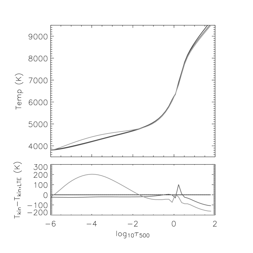
Figure 1: Temperature ($T_{\rm kin}$) structure of theoretical atmospheric models of the Sun as a function of continuum optical depth at 500 nm ($\tau_{500}$), computed with: LTE (dark line), light metals in NLTE (NLTE_Light) (medium line), light metals and Fe -group elements in NLTE (NLTE_Fe) (light line). Upper panel: Absolute $T_{\rm kin}$, lower panel: $T_{\rm kin}$ relative to that of the LTE model; dotted line: 0 K.

Fig. 1 shows the computed kinetic temperature ($T_{\rm kin}$) structure for all of the solar models as a function of the logarithm of the optical depth due to continuous opacity at 500 nm ($\log\tau_{500}$). We have also plotted the depth-wise temperature difference between the models and the LTE model. The triangular kinks in the $T$ differences that are seen in the lower panel around $\log\tau_{500}\approx 0$ are due to an inflection in the LTE $T_{\rm kin}$ structure where the NLTE $T_{\rm kin}$ distribution crosses the LTE distribution twice within a narrow range of $\log\tau_{500}$. Late-type dwarf atmospheres are expected to be close to LTE because of the relatively large influence of collisions with respect to the radiation field in controlling the equilibrium state of the gas in a relatively compressed, cool atmosphere. We find the NLTE deviations in $T_{\rm kin}$ are everywhere less than 250K. The $T_{\rm kin}(\log\tau)$ structure of the NLTE_Fe model has a larger and more depth dependent deviation from the LTE model than does the NLTE_Light model. It is $\approx$ 150 K cooler than the LTE model at the bottom of the photosphere ($\log\tau\approx 2$), is warmer than the LTE model by as much as 200 K in the range $-5<\log\tau<-2$, and is has steeper surface cooling at $\log\tau<-5$.

NLTE effects in line formation have an effect on the equilibrium structure of the atmosphere by way of the requirement of radiative equilibrium. The deviation that arises is a result of the combination of many factors: that some fraction of line photons are scattered rather than thermally absorbed and emitted, thereby reducing the line’s effectiveness as a coolant near the depth of formation; that the depth at which the line source functions become thermalized is altered by the presence of scattering, and that the depth of formation of lines is altered by changes in line opacity that arise due to NLTE effects on population number, both of which alter the depth at which a line is an effective coolant; and that the intensity at line center is altered by NLTE changes in the value of the line source function. In the case of the NLTE_Fe model, the well-known LTE line blanketing effect of back-warming is slightly reduced in the $-4<\log\tau<2$ range, making for a slightly shallower $T_{\rm kin}$ structure. At the same time, the well-known effect of line cooling near the surface is enhanced (see Anderson (1989) for a detailed discussion of NLTE line formation effects on the radiative equilibrium of the Sun, and Mihalas (1978) for a basic discussion of LTE and NLTE effects of lines on theoretical atmospheric structure).

3.1.1 Comparison with other models

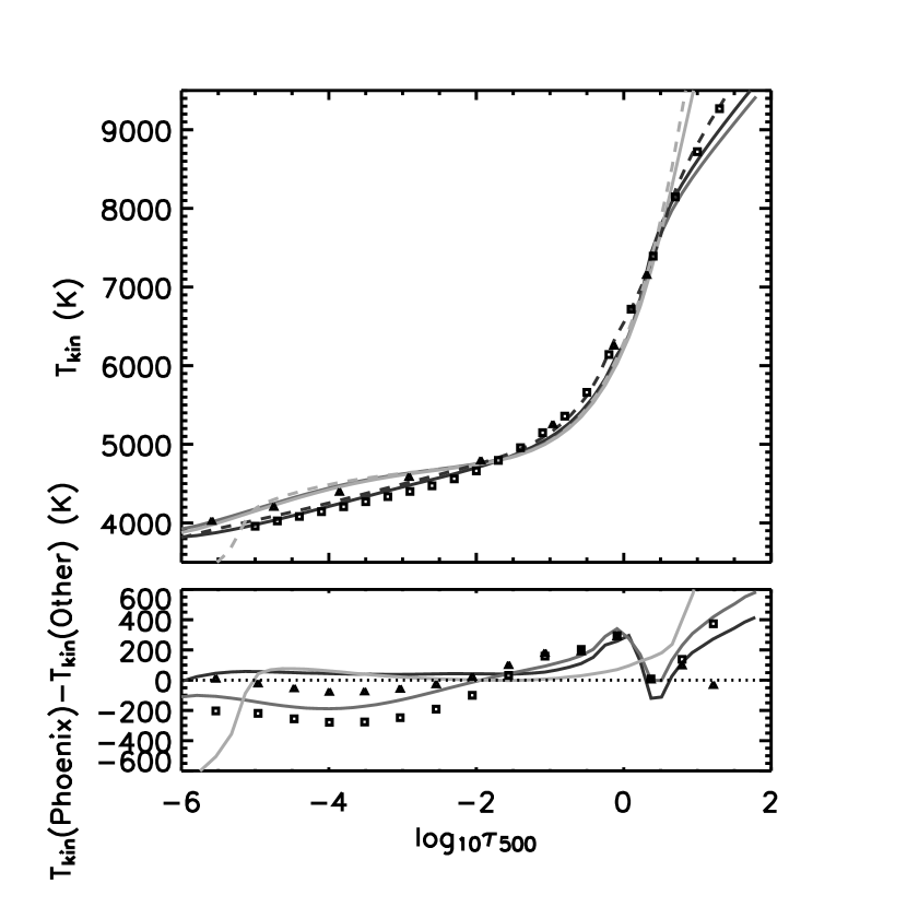
Figure 2: Temperature ($T_{\rm kin}$) as a function of continuum optical depth at 500 nm ($\tau_{500}$) of atmospheric models of the Sun from various sources. Theoretical models of other authors: dashed lines; PHOENIX models with parameters corresponding to those of other authors: solid lines. Dark lines: ASUN and LTE models with parameters of Kurucz (1992a), medium lines: NLTE_Fe models with parameters of Kurucz (1992a), light lines: PAM and NLTE_Fe with parameters of Anderson (1989). Semi-empirical models of: Holweger & Mueller (1974) (HOLMUL): triangles, and of Grevesse & Sauval (1999) (HOLMUL’): squares. Upper panel: Absolute $T_{\rm kin}$, lower panel: Difference between $T_{\rm kin}$ of other author and that of corresponding PHOENIX model; dotted line: 0 K.

Fig. 2 shows the comparison between the $T_{\rm kin}(\log\tau_{\rm 500})$ structure of our models and that of four seminal models from other investigators: the LTE model of Kurucz (1992a) computed with the ATLAS9 code (designated ASUN), the NLTE line blanketed model of Anderson (1989) computed with the PAM code (designated PAM), the LTE semi-empirical model of Holweger & Mueller (1974) (designated HOLMUL), and a modification of the HOLMUL model of Grevesse & Sauval (1999) (designated HOLMUL’). To facilitate this comparison we re-calculated our PHEONIX models with the values of $[{{\rm Fe}\over{\rm H}}]$ and “secondary” stellar parameters ($l/H_{\rm P}$ and $\xi_{\rm T}$) used by the authors of these other models. Table 3 shows the values of these parameters used for each of the comparisons. Differences among the $T_{\rm kin}(\log\tau_{\rm 500})$ structures will reflect not only differences in the equilibrium $T_{\rm kin}(r)$structure computed by each set of investigators, but also differences in the computed value of the continuous opacity at 500 nm at each depth, $\chi_{\rm c,500}(r)$,and hence in $\tau_{\rm 500}(r)$. However, both are relevant to the prediction of the emergent flux, so a comparison of $T_{\rm kin}(\log\tau_{\rm 500})$ is relevant.

ASUN:

The ASUN model is a purely theoretical LTE model that was calculated with the ATLAS9 atmospheric modeling code Kurucz (1992a). The atomic and molecular data for line blanketing opacity that is input to our PHOENIX calculation is that of ATLAS9. Therefore, the comparison to ASUN is an indicator of differences that arise due to the methodology and implementation of the solution to the LTE atmospheric modeling problem. The difference between our LTE model and ASUN is less than 100 K for $\log\tau_{\rm 500}$ values greater than 0. Near the bottom of the model the difference approaches 400 K. However, near the bottom of the model the $T_{\rm kin}(\log\tau)$ structure becomes steep so that small differences in the slope lead to large $T_{\rm kin}$ differences at a particular depth. Furthermore, the $T_{\rm kin}$ structure near the bottom of the model is affected by the treatment of convection, which, in the PHOENIX model, carries a significant fraction of the flux below $\log\tau\approx 0.18$. We emphasize again that the PHOENIX models that we are comparing with ASUN have been computed with the same value of $l/H_{\rm P}$ used to compute the ASUN model, $1.25$.

PAM:

The only previous theoretical model of the solar atmosphere with many transitions, including those of Fe  in NLTE is that of Anderson (1989), who used the PAM code. This modeling is based on a much more approximate treatment of the NLTE rate equations that the approach used here (the multifrequency/multigray algorithm). Anderson (1989) found that $T$ increased by as much as $\approx 100$ K in the $-5<\log\tau_{500}<-3$ range (his opacity scale) in NLTE, in general agreement with our NLTE_Fe results. From of Fig. 2 we find that our NLTE_Fe model agrees closely with PAM, deviating by by less than 100 K in the $-5<\log\tau_{500}<0$ range. This is a very significant result given the large differences in the way in which PHOENIX and PAM treat the NLTE SE problem. Based on a careful analysis of each type of transition’s contribution to the radiative equilibrium, Anderson (1989) concluded that strong Fe transitions dominate the thermal equilibrium in this range. Anderson (1989) also found, as we do, a sharper drop off in $T$ in the $-6<\log\tau_{500}<-5$ range than in LTE, which he attributed to CO cooling. However, a comparison to our modeling is difficult because the models of Anderson (1989) extend to $\log\tau_{500}=-8.5$ and we treat CO in LTE.

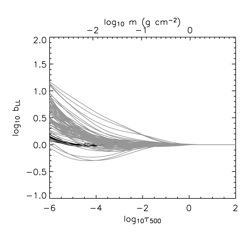
Figure 3: Ratio of upper to lower level NLTE departure co-efficients $b_{\rm LL}=b_{\rm u}/b_{\rm l}$ for select transitions of Fe II that fall within the model states f (dark lines) and g (light lines) of Anderson (1989). Lower $x$-axis: $\log\tau_{\rm 500}$ for consistency with Figs. 1, 2, and 10. Upper $x$-axis: logarithm of column mass density for comparison with Fig. 11a of Anderson (1989).

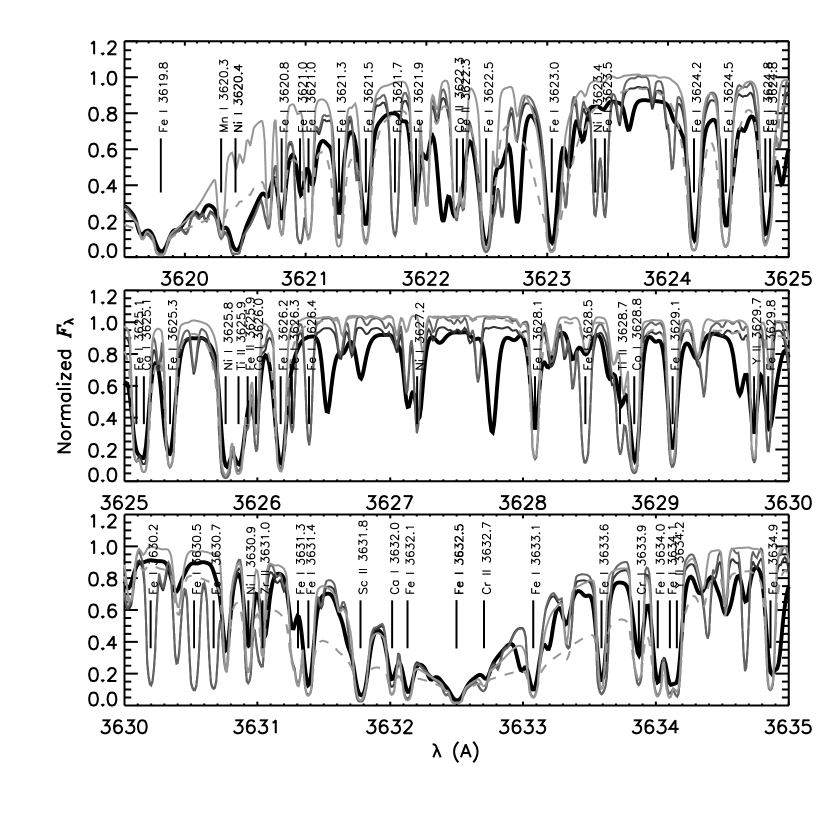
Figure 11: Comparison of observed solar flux (Kurucz et al., 1984) (thick black line) in the 3620 to 3635 Å  region (just below the Balmer jump) and synthetic spectra computed with the LTE model (thin dark line), NLTE_Light (medium line) and NLTE_Fe (light line) models with no $\gamma_{6}$ enhancement, and with the NLTE_Fe model with a $\gamma_{6}$ enhancement factor of 1.8 (dashed line).

In Fig. 11a of Anderson (1989) the long dashed lines show the ratio, $b_{\rm LL}$, of the departure coefficient of the upper level, $b_{\rm u}$, to that of the lower level, $b_{\rm l}$, for select permitted transitions of Fe II, that take place within the f and g model states of Anderson’s formalism. (For transitions that fall with a model state, Anderson calculates $b_{\rm LL}$ (also denoted in Anderson (1989) as $b_{\rm ul}$) values using the Equivalent Two Level Atom (ETLA) formalism; see Eq. 28 and 29 of Anderson (1989)). The NLTE departure co-efficient of an excitation state, $b_{\rm i}$, is defined to be the ratio of the actual occupation number of the state, $n_{\rm i}$ to that that it would have if calculated with an LTE distribution, $n_{\rm i}^{*}$ (the Boltzmann excitation and the Saha ionization distributions with excitation and ionization temperatures equal to the local thermal temperature). An important qualification for the definition of $b_{\rm i}$ used both in PHOENIX and in PAM is that $n_{\rm i}^{*}$ is calculated using the actual NLTE values of both the electron density ($n_{\rm e}$) and the ground state occupation number of the next higher ionization stage. The significance of the ratio $b_{\rm LL}$ is that it measures the amount by which the population ratio of two levels within an ionization stage departs from the local Boltzmann ratio, and is thus insensitive to NLTE departures in the ionization balance. We have re-created Anderson’s quantity $b_{\rm LL}$ for our models by extracting the departure co-efficients, $b_{\rm i}$, from the PHOENIX output for excitation states of Fe II that would qualify as falling within Anderson’s model states f and g (defined by the energy level with respect to the ground state, $\chi$, being within the range 4.0 to 5.5 $\times 10^{4}$ cm^-1, and 6.0 to 8.0 $\times 10^{4}$ cm^-1, respectively) that are connected by permitted transitions, and calculating the ratios $b_{\rm LL}=b_{\rm u}/b_{\rm l}$. These ratios are shown as a function of depth in Fig. 3, which may be directly compared to Anderson’s Fig. 11a. To facilitate the comparison, the $x$-axis has been graduated with the logarithm of column mass density, $\log m$, as well as $\log\tau_{\rm 500}$. Note that for a gas in LTE $b_{\rm LL}$ would equal unity everywhere. Unfortunately, Fe II is the only species for which Anderson provides the mapping of actual transitions to model states (Fig. 2 of Anderson (1989)), so we were unable to perform a similar comparison for Fe I. Nevertheless, our quantities $b_{\rm LL}$ for Anderson’s Fe II f and g model states show the same qualitative behavior as do Anderson’s: under-population of upper levels with respect to lower levels for some transitions as compared to LTE in the depth range $-2.5<\log m<-1$ by factors of as low as 0.4 dex, and over-population for all transitions at depths of $\log m<-2.5$ by factors approaching 1.0 dex. For some of our transitions the ratio $b_{\rm LL}$ reaches higher values than those of Anderson (1989). However, we note that Anderson’s value reflects the statistical equilibrium computed for one model state that represents the collective behavior of all the transitions shown in our Fig. 3.

Semi-empirical models HOLMUL and HOLMUL’:

Ideally, theoretical models should match semi-empirical models, although we do not expect such a match with our models because of the amount of physics that has been neglected (see section 2.1). Nevertheless, the importance of the neglected physics can be estimated by assessing the quality of match to theoretical models of limited realism. The temperature structure of the HOLMUL model was inferred from fits of LTE $F_{\lambda}$ and intensity ($I_{\lambda}$) distributions to spectral line profiles and the continuum intensity at disk center and near the limb. Although HOLMUL is an LTE model, we have chosen to compare it to our NLTE_Fe model to study the difference between a semi-empirical model without a chromospheric $T$ inversion and our most realistic theoretical model in radiative-convective equilibrium. In any case, it can be seen from the upper panel of Fig. 2 that HOLMUL is in closer agreement to our NLTE_Fe model than to our LTE model throughout the upper atmosphere. Indeed, HOLMUL deviates from our NLTE_Fe model by less than 100 K in the $-6<\log\tau_{500}<-1.5$ range. Again, the largest differences are near the bottom of the model where the $T_{\rm kin}(\log\tau)$ becomes steep and convection plays a role. The HOLMUL’ model is an adjustment made to HOLMUL by Grevesse & Sauval (1999) to reconcile solar $[{\rm Fe}/{\rm H}]$ values derived from low and high excitation Fe I lines. It is systematically 200 K cooler than HOLMUL throughout the upper atmosphere. From the upper panel of Fig. 2 we note that HOLMUL’ provides a much closer to fit to our LTE $T_{\rm kin}$ structure than to our NLTE_Fe structure above a $\log\tau_{\rm 500}$ of -1.5.

It is noteworthy that of the two semi-empirical models, one closely tracks the NLTE_Fe and the other the LTE theoretical model throughout the upper atmosphere. We emphasize again that HOLMUL’ is based on an LTE calculation of the Fe line strengths, whereas HOLMUL is based on a wider variety of diagnostics, including center-to-limb variation. Therefore, this is possibly a demonstration of the “self-fulfilling prophecy” nature of adopting LTE versus NLTE in the treatment of Fe in semi-empirical models as described by Rutten (1986).

3.2 Absolute flux distribution

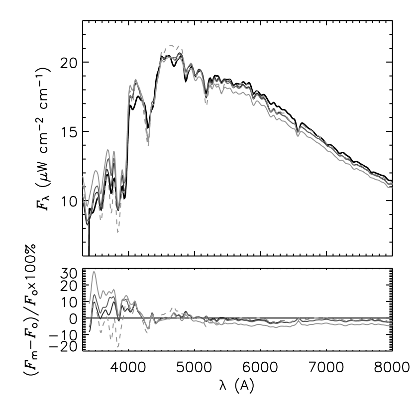
Figure 4: Comparison of the absolute global flux distribution ($F_{\lambda}(\lambda)$) of the Sun measured by Neckel & Labs (1984) (thick black line) and synthetic distributions computed for LTE (dark line), NLTE_Light (medium line), and NLTE_Fe (light line) models, the latter with a $\gamma_{6}$ enhancement factor of unity (solid line) and of 1.8 (dashed line). Upper panel: Absolute $F_{\lambda}$, lower panel: the difference between the model ($F_{\rm m}$) and observed ($F_{\rm o}$) $F_{\lambda}$ distributions, as a percentage of $F_{\rm o}$.

Fig. 4 shows the comparison of the observed solar flux distribution, $F_{\lambda}(\lambda)$, as measured by Neckel & Labs (1984) and the model flux distributions. We also show the deviation of the computed flux from the observed flux as a percentage of the observed flux. We have re-sampled and convolved the Neckel & Labs (1984) data so that it has a uniform $\Delta\lambda$ of 50Å. We also convolved our medium resolution ($R=200\,000$) synthetic $F_{\lambda}$ distribution with a Gaussian of a FWHM value of 50 Å  to facilitate the comparison.

The LTE and NLTE models are in close agreement with the observed $F_{\lambda}$ distribution on the Rayleigh-Jeans side of the solar $F_{\lambda}$ distribution where line blanketing is less severe. However, all models become increasingly discrepant with the observed flux for $\lambda\stackrel{{\scriptstyle<}}{{\sim}}5500$ Å  where the $F_{\lambda}$ distribution is increasingly affected by line blanketing. Both errors in the atomic parameters that affect line formation, and errors in the physics of line formation, have an increasingly large effect on the computed $F_{\lambda}$ distribution with decreasing $\lambda$ due the increasing line opacity. While the former source of error is presumably random, the latter may be systematic. Indeed, in the $3500<\lambda<5000$ Å  region the more realistic NLTE models provide a fit that is increasingly worse than the LTE models as the level of NLTE realism is increased. Whereas the LTE model systematically over-predicts $F_{\lambda}$ by less than $10\%$ for $\lambda<4500$Å, the NLTE_Fe model over-predicts $F_{\lambda}$ by as much as $30\%$. This may indicate that the adoption of LTE masks some other inadequacy in the models. One possibility is that, despite the addition of tens of millions of theoretical lines by Kurucz (1992a), the model opacity is still incomplete in the UV band.

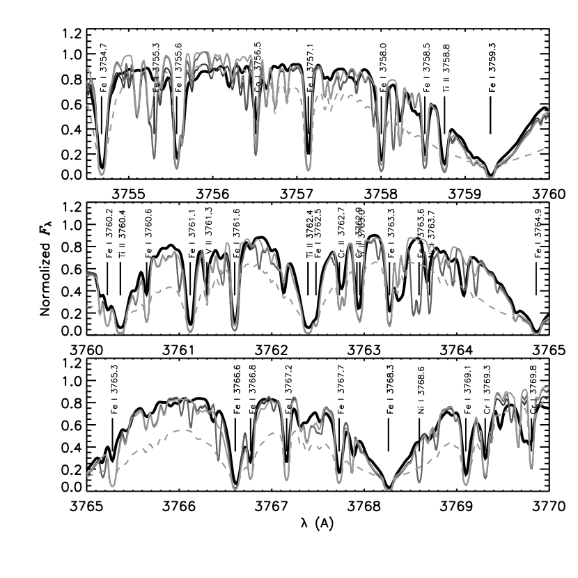
Figure 12: Same as Fig. 11, but for 3755 to 3770Å  region.

In this regard it is important to note that the treatment of line broadening has a significant effect on the calculated $F_{\lambda}$ level on a broad-band scale because of the collective effect of damped lines on the emergent flux, especially in the heavily blanketed UV region. Our value of the $VW$ broadening enhancement parameter, $E_{6}$, which is taken to be the same for all lines, has been tuned to provide a close match to the wing profiles of many damped lines in the solar spectrum (see Section 3.3 and Figs. 11 and 12). We have found that we get the best fit to the profiles of damped lines by adopting an enhancement factor of unity. This very interesting point is elaborated upon in Section 3.3. As a result, the collective opacity of damped lines in our spectrum synthesis is smaller than that of previous calculations such that our calculated $F_{\lambda}$ is larger than that computed by other investigators using the same atmospheric parameters. For comparison purposes, we have also calculated an LTE spectrum with a more traditional enhancement factor of 1.8 and shown it in Fig. 4. As expected, the introduction of the enhancement factor depresses $F_{\lambda}(\lambda)$ in the UV such that the LTE model under-predicts $F_{\lambda}$ there. We find that an LTE model of canonical solar atmospheric parameters provides a closer fit to $F_{\lambda}(\lambda)$ with an $E_{6}$ value of unity (ie. no enhancement), which is consistent with our result that the enhancement is not needed to fit the detailed line profiles.

Near UV band:

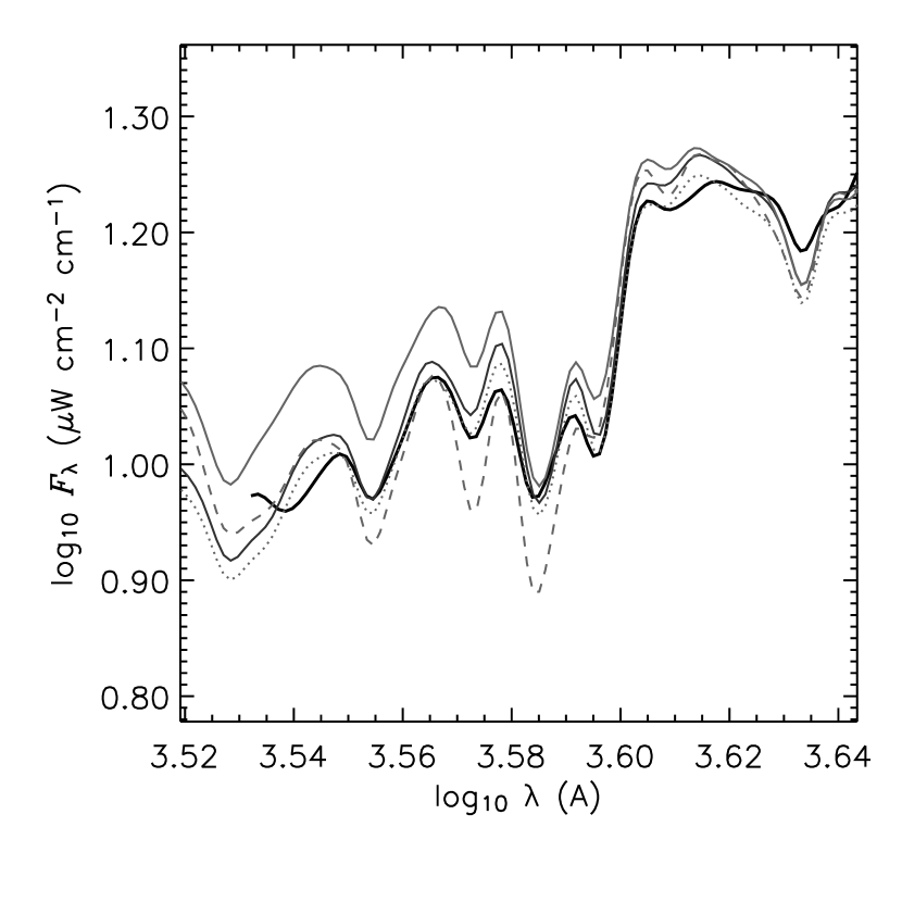
Figure 5: Comparison of observed Neckel & Labs (1984) (thick black line) and computed violet and UV band logarithmic flux distributions ($\log F_{\lambda}(\log\lambda)$). Theoretical distributions are shown for LTE (thin dark line), NLTE_Light (medium line), and NLTE_Fe (light line) models. LTE spectrum synthesis with NLTE_Fe model: dotted line, NLTE_Fe spectrum synthesis with $\gamma_{6}$ enhancement factor of 1.8: dashed line.

Fig. 5 shows the comparison of the observed and the computed $\log F_{\lambda}(\log\lambda)$ distributions in the $\lambda<5000$ Å  region. Discrepancies between the computed $F_{\lambda}$ distributions and the observed distribution, and among the computed $F_{\lambda}$ distributions themselves, are largest in this region. It should be noted that traditionally solar models have been too bright in the UV band, which discrepancy has been described as the “UV flux problem” (Kurucz, 1990). However, Kurucz (1992a) found that solar models fit the UV band $F_{\lambda}$ distribution much better when the previous atomic line lists, which consisted mainly of lines for which atomic data had been measured in the laboratory, are supplemented by millions of theoretically predicted lines from atomic model calculations. We are using the more complete line lists of Kurucz (1992a) in our models.

We also computed $F_{\lambda}$ in LTE with the NLTE_Fe model as input. Such a calculation is internally inconsistent, but allows us to assess the relative importance of direct NLTE line formation effects and indirect NLTE atmospheric structure effects in accounting for the difference between the LTE and NLTE_Fe UV $F_{\lambda}$ distributions. The resulting $F_{\lambda}$ distribution is also shown in Fig. 5, where it can be seen that it differs negligibly from the self-consistent $F_{\lambda}$ distribution computed with the LTE model. This indicates that it is direct NLTE effects on the line formation through the radiative transfer and statistical equilibrium that account for most of the difference between the $F_{\lambda}$ distributions of the LTE and NLTE_Fe models, rather than the differences in the atmospheric structure. Given the small extent of NLTE deviation seen in Fig. 1 this is not surprising. Finally, we also computed LTE and NLTE_Fe $F_{\lambda}(\lambda)$ distributions using the HOLMUL’ model for the input atmospheric structure. Because HOLMUL’ is cooler than our LTE model by as much as $\sim 100$ K at $\log\tau$ values less than -1, it is expected to yield a fainter UV band $F_{\lambda}$ level. However, we found that the $F_{\lambda}(\lambda)$ computed with HOLMUL’ differed negligibly from that computed with the PHOENIX models, for both the LTE and NLTE_Fe set-up. The negligible difference in predicted $F_{\lambda}(\lambda)$ reflects the small difference in the $T_{\rm kin}$ structures throughout the outer atmosphere among the models.

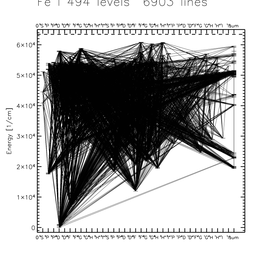
Figure 8: Grotrian diagram of the model Fe I atom used in our NLTE calculations.

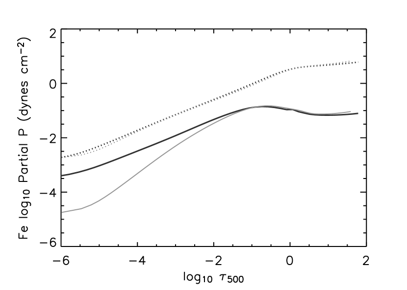
Figure 9: Partial pressure of Fe I (solid line) and  II (dotted line) in the solar LTE (dark line) and the NLTE_Fe (light line) models.

The reason for the increased UV flux in the case of the NLTE_Fe models can be seen in Figs. 8, 9, and 10. Because of its rich term structure, Fe contributes a significant fraction of the total line opacity, particularly in the UV band. Singly ionized Fe is the dominant stage, but in the LTE model Fe II/Fe I is less than ten throughout the outer atmosphere. Therefore, despite its minority status, Fe I contributes significant opacity, as a perusal of the line identifications in Figs. 11 to 13 shows. As can be seen in Fig. 10, the departure co-efficients, $b_{\rm i}$, including that for the ground state, are less than unity throughout much of the atmosphere. We emphasize again that these $b_{\rm i}$ values are with respect to $n_{\rm i}^{*}$ values that are computed with the actual value of $n_{\rm e}$ and ground state population of the next higher ionization stage (see section 3.1.1). Therefore, Fig. 10 indicates that Fe is over-ionized with respect to the LTE case. As a result, all the Fe I lines are weakened with respect to the LTE case such that the total opacity is reduced, particularly in the UV. Therefore, $F_{\lambda}$ is larger in the UV as compared to the LTE model. This is a well-known effect that has been found by previous independent investigations (see, for example, Shchukina & Trujillo Bueno (2001)).

3.2.1 Iron abundance and $b-f$ rates

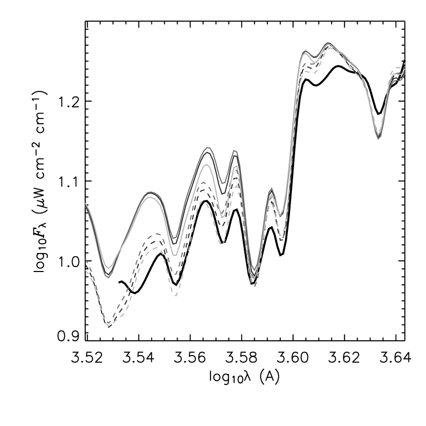
Figure 6: As for Fig. 5 except: theoretical distributions are shown for LTE and NLTE_Fe models with $[{{\rm Fe}\over{\rm H}}]$ equal to 7.5 (the originally adopted value) (dark line), 7.4 (medium line), and 7.7 (light line). LTE models: dashed line, NLTE_Fe models: solid line.

Veiling by many weak Fe I lines plays a role in determining the UV band flux of late-type stars, and the value of $[{{\rm Fe}\over{\rm H}}]$ for the Sun has been poorly constrained. To explore the effect of varying $[{{\rm Fe}\over{\rm H}}]$, we have re-calculated our models and their flux spectra with values set equal to the extrema of the range that has been recently published for the Sun, 7.4 (Holweger et al., 1990) and 7.7 (Blackwell et al., 1984). In Fig. 6 we show the resulting UV band spectra. The effect of varying $[{{\rm Fe}\over{\rm H}}]$ between the extrema is $\lambda$-dependent, being negligible at some $\lambda$ values and as much as 0.3 dex at other values. As expected, increased $[{{\rm Fe}\over{\rm H}}]$ leads to suppression of the UV flux due to increased line blocking. However, even with maximum $[{{\rm Fe}\over{\rm H}}]$ value the flux from the NLTE_Fe model is still significantly larger than that observed.

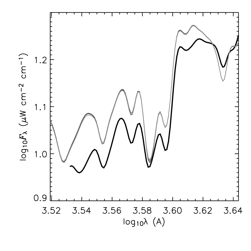
Figure 7: As for Fig. 5 except: theoretical distributions are shown for NLTE_Fe models with $\sigma_{\rm b-f,Rad}$ and $\sigma_{\rm b-f,Col}$ for all Fe -group elements equal to Opacity Project or Allen (1973) values, respectively (dark line), decreased by a factor of three and ten, respectively (medium line), and increased by a factor of three and ten, respectively (light line).

A complication that can compromise the value of NLTE modeling is that the solution is dependent on a larger variety of atomic data than is an LTE model, and these data are often uncertain by an order of magnitude or more. In the case of NLTE Fe I over-ionization and the resulting UV flux level, the cross-section for both radiative and collisional ionization are important. To investigate the dependence of our models on these rates we have calculated two variations on the NLTE_Fe model; one in which the cross-sections for radiative and collisional $b-f$ processes, $\sigma_{\rm b-f,Rad}$ and $\sigma_{\rm b-f,Col}$, for all neutral stage Fe -group elements are increased by factors of three and ten, respectively, and another in which they are decreased by a factors of three and ten. These perturbation factors adopted are the same as those adopted by Shchukina & Trujillo Bueno (2001). These two models represent the two conspiracies of error that would have maximum effect (eg. all rates for all neutral Fe -group species being maximally underestimated). In Fig. 7 we show the resulting spectra in the UV band. It can be seen that the perturbation affects the spectra negligibly, and cannot explain the discrepancy with the observed spectrum.

3.3 Moderately high resolution spectrum

Figs. 11 to 13 show the comparison between the observed flux spectrum as measured by Kurucz et al. (1984) and medium resolution synthetic spectra computed with our LTE and NLTE models for three 15 Å  bands throughout the UV and violet spectral region. The plots are annotated with the identity of the strongest line at each wavelength where there is significant line opacity.

The synthetic spectra of all models were rectified by division by a pure continuum spectrum that was synthesized with line opacity excluded with the corresponding model. We compare the observed and computed spectra at a resolution, $R$, of 200 000 to emulate the typical quality of the data for solar type stars. Our purpose here is to assess the overall fit to typical observed stellar spectra rather than to fit subtle details such as isotopic shifts or hyper-fine splitting. To ensure accurate registration for $\lambda$-wise differencing, the $\lambda$ scale of the synthetic spectrum was empirically re-calibrated with a linear dispersion relation, the coefficients of which were determined by minimizing the RMS deviation between our high resolution $F_{\lambda}$ distribution as computed with the LTE model and the observed solar flux spectrum. We note that the Sun has a $v\sin i$ value of 2 km s^-1 that should be taken into account in our synthetic spectra. However, computational constraints limit our NLTE spectrum synthesis to $R$ values that are too small for meaningful convolution with a kernel of 2 km s¹ width. However, we restrict our analysis to a discussion of spectral features on a scale that is more gross than that of rotational broadening, and to a strictly differential comparison of LTE and NLTE fits.

An inspection of the identities of the lines in Fig. 11 through 13 reveals immediately why the NLTE_Fe models differ from the LTE models much more than the NLTE_Light models do. Almost every line strong enough to meet our criterion for being labeled, including almost all the lines with extended damping wings, is an Fe I line, and the remainder are largely Fe -group lines. Furthermore, there is an unlabeled veil of weak Fe I lines that collectively serves as a pseudo-continuous opacity in the UV. This pervasiveness and dominance of Fe opacity in the violet and near UV bands is a well known phenomenon. Clearly, proper treatment of the NLTE Fe I excitation equilibrium and the Fe I/Fe II ionization equilibrium are of dominant importance for accurate modeling of this region. Of secondary importance are other Fe -group elements such as Ti, Cr, and Ni. We note that the first two ionization stages of Ti, Mn, Co, and Ni are included in the NLTE treatment in our NLTE_Fe models.

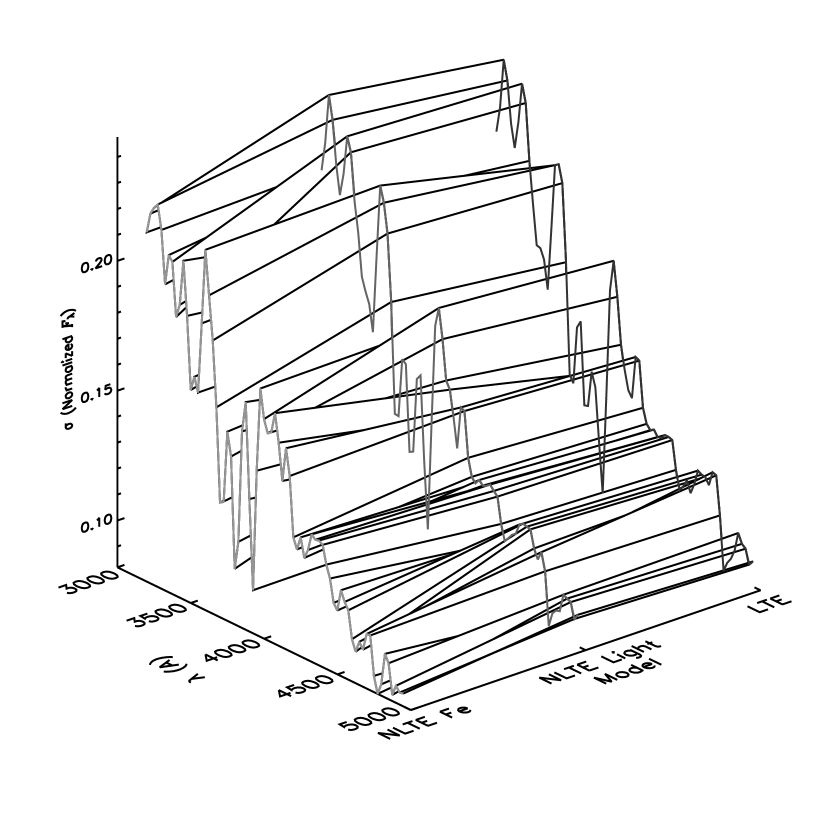
Figure 14: RMS deviation ($\sigma$) of the computed high resolution rectified flux distribution ($F_{\lambda}(\lambda)$) from the high resolution spectrum measured by Kurucz et al. (1984) in the UV and blue bands, as calculated for a running 50Å  window. Deviations are shown for the LTE (dark line), NLTE_Light (medium line), and NLTE_Fe (light line) models.

Fig. 14 shows the RMS deviation ($\sigma$) of the rectified moderately high resolution model spectra from the observed flux spectrum for the LTE and NLTE models as calculated for a 50Å  running mean throughout the 3200 to 5000Å  range. It can be seen that the quality of the fit for all models deteriorates significantly toward shorter $\lambda$ values. The reason is that the density of spectral lines increases with decreasing $\lambda$. As a result, the quality of the fit becomes increasingly sensitive to deficiencies in both the line list and the physical realism with which line formation is modeled. Also, as $\lambda$ decreases below the Wien peak of the black-body distribution for the Sun’s $T_{\rm eff}$ (5000 Å) the absolute $F_{\lambda}$ value becomes increasingly sensitive to the temperature structure of the model atmosphere, and this may indirectly effect the line formation. Finally, although the pseudo-continuum does not go completely into emission until $\lambda<2500$ Å, an increasing number of strong lines may have chromospheric emission in their cores as $\lambda$ decreases.

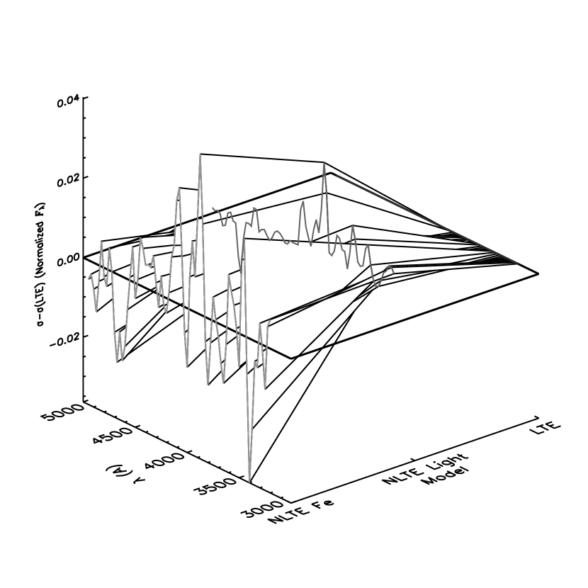
Figure 15: As for Fig. 14, but with the RMS deviation ($\sigma$) normalized by $\lambda$-wise subtraction of $\sigma$ for the LTE model. Note that, to allow the clearest view of the $\sigma$ surfaces, the wavelength ($\lambda$) axis in this figure is reversed with respect to that of Fig. 14.

Fig. 15 contains similar plot, in which the steep global $\lambda$ dependence of the $\sigma(\lambda)$ surface has been removed by $\lambda$-wise subtraction of the $\sigma(\lambda)$ values of the LTE model, $\sigma(\lambda)-\sigma(\lambda,LTE)$. Fig. 15 allows a direct assessment of how well the fit of each model compares to that of the LTE model as a function of $\lambda$. Note that, to make the entire $\sigma$ surface visible, the $\lambda$ axis has been reversed with respect to that of Fig. 14. It can be seen that $\sigma-\sigma(LTE)$ for the NLTE synthetic spectra are scattered within $\pm\approx 0.02$ rectified continuum units of that of the LTE model. This indicates that the NLTE spectra provide a better fit to the detailed shape of the moderately high resolution observed spectrum at some $\lambda$ intervals, and a worse one at others. The NLTE_Fe spectrum shows a larger range of $\sigma-\sigma(LTE)$ than does the NLTE_Light spectrum, which indicates that inclusion of Fe -group elements in the NLTE SE exaggerates further still the goodness of fit at some $\lambda$ intervals, and the badness of the fit at others. However, given that $\sigma-\sigma(LTE)<0.02$ at most $\lambda$ points, we may conclude that both NLTE synthetic spectra give a fit to the detailed shape of the observed spectrum that does not differ significantly from that of the LTE spectrum. We conclude that, within the limits of our modeling, globally fitting the detailed shape of the spectrum is not as good a test of NLTE models as fitting the overall flux level.

3.3.1 van der Waals broadening

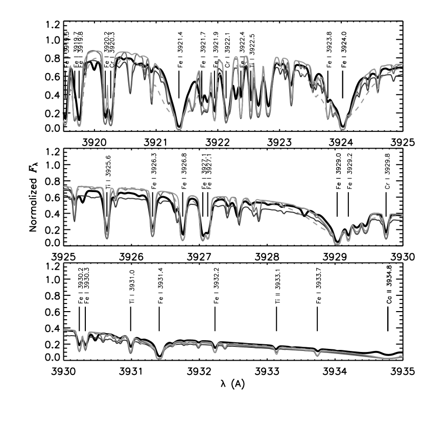
Figure 13: Same as Fig. 11, but for 3920 to 3935Å  region. The broad absorption line that spans the lowest two panels is the Ca II $K$ line.

Voigt profiles were calculated for the spectral lines that take into account van der Waals (VW) broadening due to collisions with H I, which dominates the line broadening in the solar atmosphere. The VW broadening parameter, $\gamma_{6}$, is calculated with the Unsoeld approximation (Unsoeld, 1955). To fit the profiles of damped lines, many previous investigators find it necessary to enhance the value of $\gamma_{6}$, ad hoc, by an arbitrary factor, $E_{6}$, that usually ranges from 1 to 3 (see Kostik et al. (1996) for a detailed discussion). The physical meaning of the enhancement is unclear, and one possibility is that, like micro-turbulence ($\xi_{\rm T}$), it is at least partially a “fudge” factor to account for inhomogeneities in the solar (or stellar) atmosphere (Shchukina & Trujillo Bueno, 2001). We have computed our spectra with an $E_{6}$ value of unity; ie. no enhancement. We also show in Figs. 11 through 13 a spectrum computed with the NLTE_Fe model and a more traditional $E_{6}$ value of 1.8, which provides a closer match to the observed $F_{\lambda}$ level (see section 3.2. It can be seen that in the near UV band, the traditional enhancement gives computed line profiles that are systematically too broad, whereas, an enhancement factor of unity provides a close match to all the damped lines. The only exception is the very broad Ca II $\lambda 3934.8$ line (Fig. 13), which is equally well fit with both values of $E_{\rm 6}$.

For any other star, one might argue that the necessity of neglecting the $\gamma_{6}$ enhancement is masking an inadequacy in the model that exaggerates the pressure broadening, such as an adopted value of $\log g$ or $[A/H]$ that is too large. However, in the case of the Sun the atmospheric parameters are known to very high precision. It is noteworthy that most of the damped lines in Figs. 11 and 12 are Fe I lines. Blackwell et al. (1995) found that the value of $E_{6}$ that provides the best fit to Fe I lines in the visible band depends on multiplet number, with lines arising from multiplet numbers less that 50 having best fit $E_{6}$ values less than 1.1. In the 3000 to 4000 Å  band, 26 out of about 140 Fe I lines of $\log gf$ value greater than -1 listed in the NIST multiplet table arise from multiplet numbers less than 50. Similarly, Bensby et al. (2003) investigated the variation of derived abundances for F and G dwarfs with input atomic parameters and adopted a relatively low value of $E_{6}=1.4$ for Fe I lines of lower excitation potential greater than 2.6 eV. Another possibility is that the systematic over-damping of these lines in the LTE spectrum synthesis with a $\gamma_{6}$ enhancement of 1.8 is due to neglect of the NLTE over-ionization of Fe. However, comparison of the LTE and NLTE_Fe synthetic spectra in Figs. 11 and 12 shows that, while NLTE over-ionization may lift the veil of weak Fe I lines that collectively block UV flux, it is not enough to significantly weaken the profiles of damped Fe I lines.

4 Conclusions

We have presented atmospheric models and synthetic flux spectra for a late-type MS star with the parameters of the Sun, that represent three degrees of realism in the treatment of the equilibrium state of the gas and the radiation field. We have studied separately NLTE effects in Fe -group elements and light metals on the model structure and emergent flux, and the ability of these models to fit both the broad-band absolute $F_{\lambda}(\lambda)$ level and moderately high resolution spectra.

The theoretical $T(\tau)$ structure of our most realistic model (NLTE_Fe) agrees to within 100 K with both the more approximate theoretical NLTE line blanketed model of Anderson (1989) (PAM) and the LTE semi-empirical structure found by of Holweger & Mueller (1974) (HOLMUL). The LTE and NLTE_Light models are in closer agreement to the theoretical LTE model of Kurucz (1992a) and the LTE semi-empirical structure found by Grevesse & Sauval (1999) (HOLMUL’). The agreement between the NLTE_Fe model and the PAM model is remarkable vindication of the approximate multifrequency/multigray method developed by Anderson (1989). The comparison with the two LTE semi-empirical models is of particular interest: HOLMUL’ is based on an LTE analysis of the Fe I excitation equilibrium, whereas HOLMUL is based on a wider variety of spectral features and center-to-limb variation. Therefore, the former may fall prey to the “self-fulfilling prophecy” effect described by Rutten (1986): adoption of LTE in the treatment of Fe  leads to an inferred $T_{\rm kin}$ structure that produces the observed spectrum when Fe  is treated in LTE.

The NLTE effects of Fe -group elements on the model structure and $F_{\lambda}$ distribution are much more important than the NLTE effects of all the light metals combined, and serve to substantially increases the violet and near UV $F_{\lambda}$ level as a result of NLTE Fe over-ionization. Based on calculations of LTE and NLTE $F_{\lambda}$ distributions with the semi-empirical $T_{\rm kin}(\tau)$ structure of Grevesse & Sauval (1999), and on calculation of the LTE $F_{\lambda}$ distribution with the NLTE_Fe $T_{\rm kin}(\tau)$ structure, the discrepancy between the observed and predicted $F_{\lambda}$ level is much too large to be due to errors in the model structure. These results suggest that there may still be important UV opacity missing from the models. We know that nature is not obliged to be in LTE, and, therefore, on general principle, it should be modeled in NLTE. If NLTE calculations sometimes worsen the fit of models to observational data, that may serve to expose other modeling inadequacies that had been partially hidden by LTE modeling. We also find that the RMS deviation, $\sigma(\lambda)$, of the moderately high resolution synthetic spectrum from the observed spectrum is changed randomly by $\pm 0.02$ rectified continuum units by the adoption of NLTE. We conclude from the latter that within the limits of the present models, the statistical goodness of fit to many line profiles is not a good discriminator of merit between LTE and NLTE models.

The quality of the fit to the UV $F_{\lambda}$ level is sensitive to the extent to which strong lines are damped by van der Waals broadening, and the notorious vdW enhancement parameter, $E_{6}$, is species (and transition) dependent. A traditional value of $E_{6}$ of 1.8 gives a close fit to the observed $F_{\lambda}$ distribution but an unacceptably poor fit to the detailed shape of damped lines. On the other hand, a value of unity (ie. no enhancement) gives a close fit to the many damped Fe I lines in the near UV while leading to a predicted $F_{\lambda}$ distribution that is too bright.

Figure 10: NLTE departure coefficients for Fe I and  II in the solar NLTE_Fe model. The ground state coefficient is shown with a thick black line. The lighter the color of the line the higher the energy, $E$, of the level.

Table 1: Species treated in Non-Local Thermodynamic Equilibrium (NLTE) in the NLTE_Light and NLTE_Fe models. Each ionization stage is labeled with the number of energy levels and bound-bound transitions included in the statistical equilibrium rate equations. Note that this table shows only a sub-set of the total number of species that are currently treatable in statistical equilibrium by PHOENIX.

Element	Model	Ionization Stage
		I	II	III
H	NLTELight, NLTEFe	80/3160	$\cdots$	$\cdots$
He	NLTELight, NLTEFe	19/37	$\cdots$	$\cdots$
Li	NLTELight, NLTEFe	57/333	55/124	$\cdots$
C	NLTELight, NLTEFe	228/1387	$\cdots$	$\cdots$
N	NLTELight, NLTEFe	252/2313	$\cdots$	$\cdots$
O	NLTELight, NLTEFe	36/66	$\cdots$	$\cdots$
Ne	NLTELight, NLTEFe	26/37	$\cdots$	$\cdots$
Na	NLTELight, NLTEFe	53/142	35/171	$\cdots$
Mg	NLTELight, NLTEFe	273/835	72/340	$\cdots$
Al	NLTELight, NLTEFe	111/250	188/1674	$\cdots$
Si	NLTELight, NLTEFe	329/1871	93/436	$\cdots$
P	NLTELight, NLTEFe	229/903	89/760	$\cdots$
S	NLTELight, NLTEFe	146/439	84/444	$\cdots$
K	NLTELight, NLTEFe	73/210	22/66	$\cdots$
Ca	NLTELight, NLTEFe	194/1029	87/455	150/1661
Ti	NLTEFe	395/5279	204/2399	$\cdots$
Mn	NLTEFe	316/3096	546/7767	$\cdots$
Fe	NLTEFe	494/6903	617/13675	$\cdots$
Co	NLTEFe	316/4428	255/2725	$\cdots$
Ni	NLTEFe	153/1690	429/7445	$\cdots$

Table 2: Levels of modeling realism.

Degree of NLTE	Model designation
None	LTE
Light metals only	NLTELight
Light metals & Fe -group	NLTEFe

Table 3: Iron abundance and secondary stellar parameters of PHOENIX models that are compared to models of other authors.

Author/Model	$[{{\rm Fe}\over{\rm H}}]$	$l/H_{\rm P}$	$\xi_{\rm T}$ (km s-1)
Kurucz (1992a)/ASUN	7.63	1.25	1.5
Anderson (1989)/PAM	7.50	0.0	1.5

References

- Anderson (1989) Anderson, L.S., 1989, ApJ, 339, 558
- Allen (1973) Allen, C. W. 1973, Astrophysical Quantities (3d ed.; London: Athlone)
- Asplund (2000) Asplund, M., 2000, A&A, 359, 755
- Bautista, et al. (1998) Bautista, M. A., Romano, P., & Pradhan, A. K., 1998, ApJS, 118, 259
- Bensby et al. (2003) Bensby, T., Feltzing, S. & Lundstrom, I., 2003, A&A, 410, 527
- Bessell et al. (1998) Bessell, M. S., Castelli, F., Plez, B., 1998, A&A, 333, 231
- Blackwell et al. (1984) Blackwell, D.E., Booth, A.J. & Petford, A.D., 1984, A&A, 132, 236
- Blackwell et al. (1995) Blackwell, D.E., Lynas-Gray, A.E. & Smith, G., 1995, A&A, 296, 217
- Drawin (1961) Drawin, H. W., 1961, Z. Phys., 164, 513
- Grevesse et al. (1992) Grevesse, N., Noels, A., Sauval, A.J., 1992, In ESA, Proceedings of the First SOHO Workshop, p. 305
- Grevesse & Sauval (1999) Grevesse, N. & Sauval, A.J., 1999, A&A, 347,348
- Hauschildt & Baron (1999) Hauschildt, P.H. and Baron, E., 1999, J. Comp. App. Math., 109, 41
- Holweger et al. (1990) Holweger, H., Heise, C. & Kock, M., 1990, A&A, 232, 510
- Holweger et al. (1995) Holweger, H., Kock, M. & Bard, A., 1995, A&A, 296, 233
- Holweger & Mueller (1974) Holweger, H. & Mueller, E.A., 1974, Sol. Phys., 39,19
- Kostik et al. (1996) Kostik, R.I., Shchukina, N.G. & Rutten, R.J., 1996, A&A, 305, 325
- Kurucz (2002) Kurucz, R.L., 2002, in AIP Conference Proceedings, 636, No. 1, p. 134, eds. Schultz, P.S. Krstic, and F. Ownby
- Kurucz (1994a) Kurucz R.L. 1994, CD-ROM No 19 (Cambridge: SAO)
- Kurucz (1994b) Kurucz R.L. 1994, CD-ROM No 22, Atomic Data for Fe and Ni (Cambridge: SAO)
- Kurucz (1992a) Kurucz, R.L., 1992, Rev. Mex. Astron. Astrofis., 23, 181
- Kurucz (1990) Kurucz, R.L. 1990, Trans. IAU, XXB 168
- Kurucz & Bell (1995) Kurucz, R. L., & Bell, B. 1995, CD-ROM 23, Atomic Line List (Cambridge: SAO)
- Kurucz et al. (1984) Kurucz, R.L., Furenlid, I., Brault, J., National Solar Observatory Atlas, Sunspot, New Mexico: National Solar Observatory, 1984
- Mathisen (1984) Mathisen, R. 1984, Photo Cross Sections for Stellar Atmosphere Calculations: Compilation of References and Data (Inst. Theor. Astrophys. Publ. Ser. 1; Oslo: Univ. Oslo)
- Mihalas (1978) Mihalas, D., 1978, Stellar Atmospheres, W.H. Freeman & Co., p. 239
- Neckel & Labs (1984) Neckel, H. & Labs, D., 1984, Sol. Phys., 90, 205
- Plez et al. (1992) Plez, B., Brett, J. M., Nordlund, A., 1992, A&A, 256, 551
- Reilman & Manson (1979) Reilman, R. F. & Manson, S. T., 1979, ApJS, 40, 815
- Rutten (1986) Rutten, R.J., 1986, in IAU Colloquium 94, Physics of Formation of Fe II lines outside LTE, ed. R. Viotti (Dordrecht: Reidel)
- Seaton et al. (1994) Seaton, M. J., Yan, Y., Mihalas, D., & Pradhan, A. K., 1994, MNRAS, 266, 805
- Shchukina & Trujillo Bueno (2001) Shchukina, N. & Trujillo Bueno, 2001, ApJ, 550, 970
- Short & Hauschildt (2003) Short, C. I. & Hauschildt, P. H., 2003, ApJ, 596, 501
- Short et al. (1999) Short, C. I., Hauschildt, P. H., Baron, E., 1999, ApJ, 525, 375
- Thevenin & Idiart (1999) Thevenin, F. & Idiart, T.P., 1999, ApJ, 521, 753
- Unsoeld (1955) Unsoeld, A., 1955, Physik der Sternatmospharen, ed. Berlin: Springer-Verlag
- Van Regemorter (1962) Van Regemorter, H., 1962, ApJ, 136, 906