The visibility of the Galactic bulge in optical surveys. Application to the Gaia mission

The bulge is a region of the Galaxy which is of tremendous interest for understanding Galaxy formation. However, measuring photometry and kinematics in it raises several inherent issues, like high extinction in the visible and severe crowding. Here we attempt to estimate the problem of the visibility of the bulge at optical wavelengths, where large CCD mosaics allow to easily cover wide regions from the ground, and where future astrometric missions are planned. Assuming the Besançon Galaxy model and high resolution extinction maps, we estimate the stellar density as a function of longitude, latitude and apparent magnitude and we deduce the possibility of reaching and measuring bulge stars. The method is applied to three Gaia instruments, the BBP and MBP photometers, and the RVS spectrograph. We conclude that, while in the BBP most of the bulge will be accessible, in the MBP there will be a small but significant number of regions where bulge stars will be detected and accurately measured in crowded fields. Assuming that the RVS spectra may be extracted in moderately crowded fields, the bulge will be accessible in most regions apart from the strongly absorbed inner plane regions, because of high extinction, and in low extinction windows like the Baades’s window where the crowding is too severe.

1 Introduction

The bulge is an important part of the Galaxy for understanding galaxy formation and evolution, thus requiring surveys that go as deep as possible in this region. The bulge is highly extinguished at its center and at low Galactic latitudes. It also suffers from severe crowding when observed with low spatial resolution instruments. The extinction is generally very patchy. When extinction is high the crowding is less. Hence the crowding in the central regions of the Galaxy is very sensitive to the extinction and may vary strongly from field to field on a quite small spatial scale.

Observations of bulge stars will strongly depend on the extinction and on the crowding. If the extinction is too high, the number of stars will be low (no crowding) but conversely the bulge stars would not be observed, because too faint. If the extinction is low (like in the Baade’s windows), bulge giants on the red clump are bright enough to be reached, but the crowding will limit the number and/or the quality of their measurement. The number of stars in the bulge also strongly depends on latitude and longitude. Drimmel et al. (2003b) attempted to localize the densest regions from the GSC-II catalogue. The densities, as estimated from this photographic catalogue, are given for all populations together. They do not specify if bulge stars will be accessible at the Gaia limiting magnitude G$\leq$20 or not.

Here we address the following question: is there a combination of parameters (extinction, latitude) in the Galactic bulge where the extinction is large enough to avoid crowding and not too high to allow bulge star measurements in the optical ? In order to answer it, we have used the Besançon Galaxy model (Robin et al., 2003, 2004) which allows us to simulate star counts as a function of magnitude, direction and extinction. However these depend on the assumptions about Galactic structure, stellar populations and particularly the bulge model, but even more strongly on the assumed extinction. Schultheis et al. (1999) have determined a detailed map of the mean extinction in the Galactic central region $|l|<9^{\circ}$ and $|b|<1.5^{\circ}$ showing strong variations on a spatial scale of several arcminutes. The high patchiness is also visible in the Schlegel et al. (1998) map obtained from the dust column density deduced from FIR emission.

In Sect. 2 alternative extinction estimates are described. In Sect. 3 we present the Galaxy model used for this study. We briefly describe the Gaia instruments in Sect. 4. In sect. 5 we show our estimation of the magnitude of bulge stars reached as a function of the limiting G magnitude and of the extinction map, and we address the problem of the crowding in Gaia instruments. We also discuss the reliability of the results.

2 Extinction in the Galactic central regions

A fundamental parameter for estimating stellar densities in the bulge is the extinction. If the extinction is too low, the high stellar density will create heavy crowding at the limiting magnitude. If the extinction is too high the bulge stars will be too faint to be observed.

Several extinction maps have been published in the past years (Schlegel et al., 1998; Schultheis et al., 1999; Dutra et al., 2003; Drimmel et al, 2003a). Schultheis et al. (1999) (hereafter SGS) have produced a detailed analysis of the extinction at a high spatial resolution in the region -9${}^{\circ}<l<9^{\circ}$ and -1.5${}^{\circ}<b<1.5^{\circ}$. This study was made using near-infrared photometry in J and K_s bands from the DENIS survey (Epchtein et al., 1997). Isochrones of 10 Gyr and solar metallicity (Bertelli et al., 1994) have been fitted to J-K/K diagrams in 2 arcmin windows, by varying the extinction. The typical uncertainty is smaller than 2 magnitudes in windows with A${}_{V}<$25. SGS assume a fixed metallicity of Z=0.02. This corresponds to the mean value observed in red giants but a spread is known to be present in the bulge. However the effect of not accounting for this spread should not translate into a significant change in the total uncertainty. The uncertainty due to the assumed age is also negligible. In regions where A${}_{V}>$25, the measurement is no longer reliable due to the lack of detection in the J band. In this case the given value is an underestimate of the true value. In small extinction regions (Av$\approx 1$) the accuracy is limited by the sensitivity of the extinction in the K band and by the photometric accuracy which is about 0.05 in A_K, which translates to 0.5 when computing A_V. The errors in this extinction map increases towards higher extinguished regions due to the increase in photometric errors. The uncertainty on the extinction law may also contribute to the total uncertainty, especially in high extinction regions. Dutra et al. (2003) have shown that their map based on 2MASS data agrees well with the DENIS extinction map (Schultheis et al., 1999) up to $A_{K}\approx 1.5$ (about A_V=15). Above this limit, the comparison is affected by increased internal errors in both extinction determinations. However, a comparison with the Galactic center map of Catchpole et al. (1990) gives a good agreement with differences less than A_V=2 mag. The resulting map has a spatial resolution of 2 arcminutes and is the average total extinction along that line of sight to a distance of 8 kpc from the Sun.

Schlegel et al. (1998) (SFD) have produced a whole sky extinction map using FIR dust emission from IRAS and COBE/DIRBE. They obtain a high resolution map (at the resolution of IRAS) of the dust temperature and of the dust column density and calibrate the extinction estimator with a sample of elliptical galaxies. They also assume that the distribution of dust grain sizes is the same everywhere in the Galaxy and that the large grains which are responsible for the FIR emission are in equilibrium with the interstellar radiation field. The former hypothesis is only correct in diffuse medium. They also fit each line of sight with a single color temperature, which may not be true in the Galactic plane. The practical error on E(B-V) in SFD map is estimated to be 0.011 mag. However this value does not account for systematic errors in regions where their assumptions do not apply - for example in regions with high gas to dust ratios, in outflows around OB associations (Burstein, 2003). Schlegel et al. (1998) also noted that for latitudes less than 5 degrees their extinction determination is less reliable.

Comparing SGS and SFD maps in the Galactic plane leads to systematic differences. The SFD estimation is the total extinction along the line of sight through the entire Galaxy. So, in the plane, the total extinction would be about twice the value undergone by bulge stars, the difference being due to extinction on the far side of the bulge. In general in the bulge we expect SFS values to be a significative overestimate of the extinction. However at higher Galactic latitudes, this overestimate should become smaller. Moreover, because the lines of sight in the Galactic plane may encounter regions with different density and color temperatures, the SFD map is probably less reliable for estimating the extinction that bulge stars undergo. We have chosen to rely on the SGS map in regions where it exists ($|b|<1.5^{\circ}$), and on the SFD map at higher latitudes.

3 The Besançon Galaxy model

In order to estimate the total number of stars, and the number of bulge stars, in given directions as a function of magnitude, we have used model predictions from the Besançon Galaxy model (Robin et al., 2003, 2004). We describe below the main ingredients relevant to the present study.

3.1 Overview of the stellar population model

The model is based on a population synthesis scheme. Four distinct populations are assumed (a thin disc, a thick disc, a bulge and a spheroid) each deserving specific treatment. In the central regions, only the bulge and thin disc are important, the thick disc and spheroid being negligible at the magnitudes considered here.

The thin disc is a prominent population in the bulge region, especially at optical wavelengths. Although the bulge density exceeds the disc density at Galactocentric distances smaller than 3.14 kpc, the bulge is less visible due to extinction. Hence it is necessary to adequately model the foreground disc population. The density is modeled by a Einasto law with a scale length of 2.35 kpc and it develops a progressive central hole of scale length 1.32 kpc (Picaud & Robin, 2004). The maximum density of the disc is at about 2 kpc from the center. The disc population is described by an evolutionary scheme with a constant star formation rate over the past 10 Gyr. In addition, a two slope IMF has been used with a high mass slope (alpha=3), slightly higher than Salpeter’s one (Haywood et al., 1997).

3.2 The outer bulge

Picaud (2003) has undertaken a detailed analysis of the outer bulge stellar density and luminosity function by fitting model parameters to a set of 94 windows in the outer bulge situated at -8${}^{\circ}<l<10^{\circ}$ and -4${}^{\circ}<b<4^{\circ}$. The data were obtained by the DENIS survey team (Simon et al. in preparation) using K_s magnitude and J-K_s color distributions. Using a Monte Carlo method to explore a 11 dimensional space of bulge and disc density model parameters and a maximum likelihood test of goodness of fit, he showed that the bulge follows a density law which can be modeled by a boxy exponential or a boxy sech² profile. He found a triaxial bulge with the major axis pointing towards the first quadrant with an angle of about 10^∘ with respect to the Sun-Galactic center direction. A full description of the parameter values of the bulge density law can be found in Picaud & Robin (2004). Several luminosity functions have also been tested. The favoured combinations between age and evolution model are the Bruzual et al. (1997) one with an age of 10 Gyr, or the Girardi et al. (2002) one with an age of 7.9 Gyr.

In figure 1 we show the overall goodness of fit of the resulting model with a Bruzual et al. (1997) 10 Gyr luminosity function. The figure looks similar using Girardi et al. (2002) tracks, as the worse windows are the same for both stellar models. The greyscale code is a function of the square root of the $\chi^{2}$ per bin of colour-magnitude. The overall agreement is good in most of the windows except in two regions: the first one close to the Galactic center ($l=0^{\circ},b=+1^{\circ}$), an overdense region with regard to the Galaxy model which is unaccessible to optical surveys because of very high extinction; the second one being situated at around $l\approx 5^{\circ}$ and $b\approx-1.5^{\circ}$. The latter discrepancy is probably due to a bad extinction distribution model specifically in these windows.

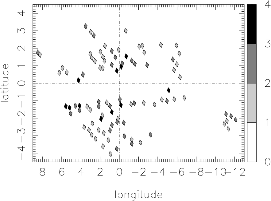
Figure 1: Overall goodness of fit of the model in 94 windows with NIR data. The greyscale is a function of the square root of the $\chi^{2}$ per bin of magnitude-colour in each window. Two regions are found at more than 3 sigmas: the first one near the bulge minor axis at $l\approx 0^{\circ}$, $b\approx 1^{\circ}$, the second one at $l\approx 5^{\circ}$, $b\approx-1.5^{\circ}$.

We will use this model to estimate the number and the absolute magnitude of bulge stars as a function of position, apparent magnitude and interstellar extinction. We also compute for the same parameters the total number of stars to address the problem of crowding.

To apply the method to Gaia instruments we have computed the G magnitude from the formula defined for the new design of the payload (Gaia-2):

$$G=V-0.00075-0.3757\times(V-I)-0.1233\times(V-I)^{2}+0.0061\times(V-I)^{3}$$

The formula is applied to V and I magnitudes reddened following the Mathis (1990) extinction law.

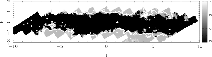
Figure 2: Absolute magnitude M_V of bulge stars just reached at magnitude G=17, as a function of latitude and longitude, according to the Schultheis et al. (1999) extinction map. An absolute magnitude of -2 means that no bulge stars are reached. The solid contour shows the iso-density of 20,000 stars per square degree, which is the crowding limit of the RVS. The regions which do not suffer from crowding with the RVS are between the dark dust lane and the iso-density contour.

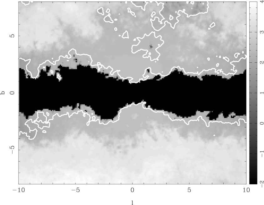
Figure 3: Same as figure 2 but using the Schlegel et al. (1998) extinction map. The white lines are isodensity contours at 20,000 total stars per square degree, the assumed crowding limit of the RVS.

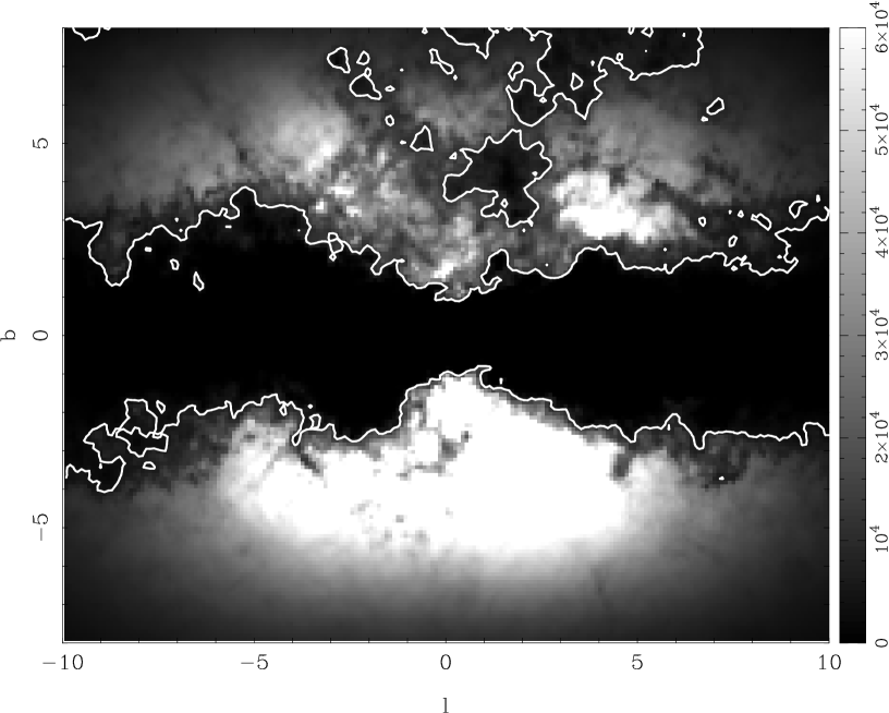
Figure 4: Bulge stellar density in stars per square degree at G $<17$ assuming the Schlegel et al. (1998) extinction map. The white lines are isodensity contours at 20,000 total stars per square degree, the assumed crowding limit of the RVS.

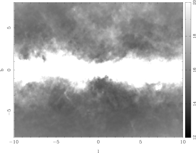
Figure 5: Apparent G magnitude at which the RVS crowding density of 20,000 stars per square degree (bulge+disc) is reached, assuming the Schlegel et al. (1998) extinction map.

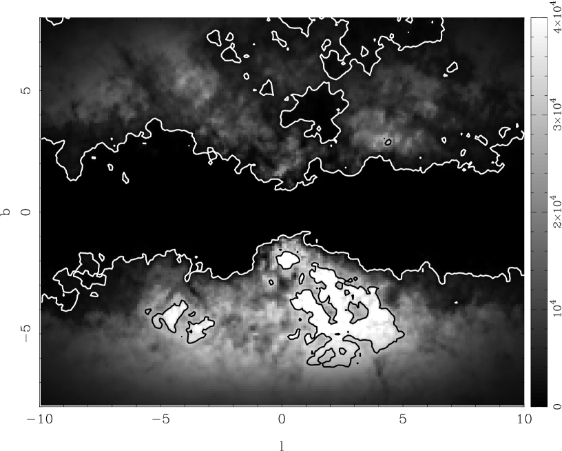
Figure 6: Bulge stellar density in stars per square degree at magnitude G $<15$, assuming the Schlegel et al. (1998) extinction map. The white lines are the isodensity contours at 20,000 stars per square degree (bulge+disc) at G$<17$, while the black lines are the same at G$<15$. Less extinguished regions at b$<$-1 (inside black contours) suffer from crowding even at G$<$15.

3.3 Reaching the bulge at magnitude 20 with the photometers

Figure 7 and 8 are similar to Figures 2 and 3 but at the limiting magnitude G=20 and for a different crowding limit of 100,000 stars per square degree.

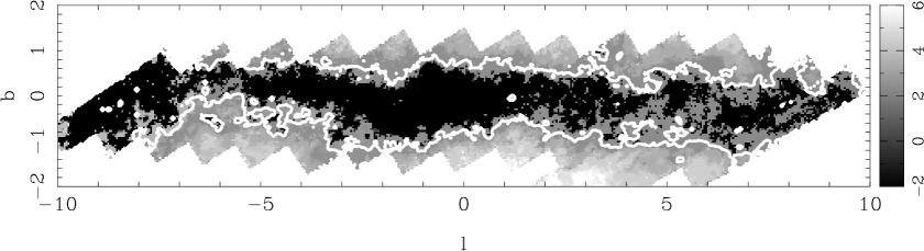
Figure 7: Absolute magnitude M_V of bulge stars just reached at magnitude G=20, as a function of latitude and longitude, according to the Schultheis et al. (1999) extinction map. An absolute magnitude of -2 means that no bulge stars are reached. The solid contour shows the iso-density of 100,000 stars per square degree, which is the crowding limit of the MBP. The region which is accessible to observation with the MBP is placed in between the dark dust lane and the iso-density contour.

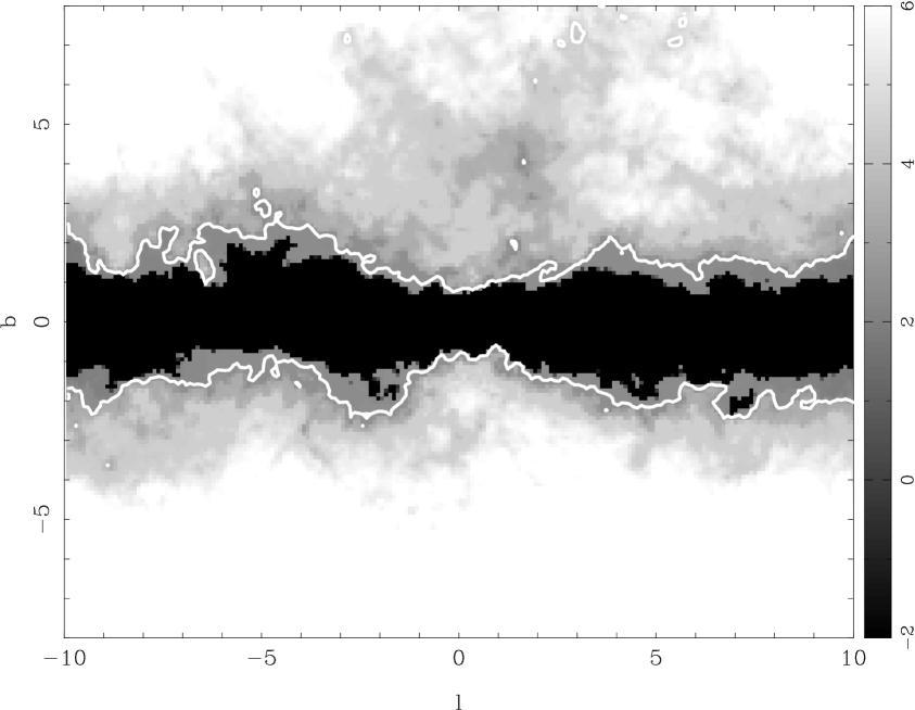
Figure 8: Same as figure 7 but using Schlegel et al. (1998) extinction map.

4 Crowding in the Gaia instruments

The crowding in Gaia instruments depends on the sensitivity and on the spatial resolution of each instrument. We shall consider each one separately.

4.1 Broad Band Photometer (BBP)

The astrometric instruments will provide accurate photometry in a few wide bands with the Broad Band Photometer (BBP) and astrometry in the Astrometric Field (AF). The pixel and sample angular areas of BBP are 44.2$\times$132.6 and 44.2$\times$1591.2 mas², respectively. The instrument qualifications have been chosen in order that it rarely reaches crowding, to be able to measure up to about 3 million stars per square degree (Jordi et al, 2002). This limit is imposed by the number of windows around each star that can be downloaded according to the telemetry budget and to the size of these windows. This may be adapted but at the price of a loss of astrometric and photometric precision at the limiting magnitude.

The sensitivity of the instrument will allow completeness upto the magnitude of about G=20. There may be a few regions in the Galactic plane and in the center of some of the globular clusters reaching this density limit (3.10⁶ stars per square degree).

4.2 Medium Band Photometer (MBP)

The Medium Band Photometer (MBP) instrument is dedicated to obtaining accurate medium band photometry in about 11 filters up to magnitude 20. The angular size of the pixel and the sample are 1$\times$1.5 arcsec² and 1$\times$6 arcsec², respectively. This means that at a density of about 270 000 stars per square degree the CCD will be completely full of stars. The crowding limit has been estimated to be between 50,000 and 100,000 stars per square degree (Hoeg, 2002) but this estimate is still under more detailed investigation. When the crowding is large in the MBP it is difficult to cross-identify a star detected in the AF and BBP with a measurement in the MBP, even for bright stars, several stars being superimposed. In the present study we have assumed a crowding limit of 100,000 stars per square degree.

4.3 Radial Velocity Spectrograph (RVS)

The Radial Velocity Spectrograph (RVS) instrument aims at observing a wavelength interval of about 26 nm around $\lambda_{c}$ = 861.5 nm. The spectral resolution has been recently chosen to be R=11500. The spectra will be 694 pixel long and 3 pixel wide (100% energy). During the Gaia mission, each target will be observed 102 times on average. Due to the scanning law, each time the orientation will be different so that if ever the star overlaps its spectrum with a neighbouring star it will not be the case in the next transit, at least not with the same star. However, in very dense fields the overlaps can happen in a significant number of transits for a given star.

Zwitter et al. (2003) have estimated the probability of overlapping between two neighbouring stars as a funtion of stellar density. The overlap appears when there is more than one star in 694 pixel length. For a stellar density of 1,200 stars per square degree at V$<$17 they found that about 21 transits in 100 are subject to overlap. Going to a density of 6,000 stars per square degree increases the fraction of overlap to about 70%.

In a complementary study Zwitter (2003) estimated how the accuracy on radial velocities may depend on the crowding. He argues that the overlaps degrade the radial velocity accuracy only at faint magnitudes (V$\>=$17.5) and in highly crowded fields. This is mainly because estimates of the overlapping spectra can be made during the Gaia survey: photometric broad band photometry and accurate astrometry will allow a first order correction of the overlapping spectra for each transit, knowing the accurate position and magnitude, and an estimate of the spectral type of the overlapping star. However the recovering of other astrophysical parameters (temperature, gravity, metallicity) will be limited to bright targets in not too dense environments.

In estimating the possibility of observing bulge stars with the RVS, we have assumed a crowding limit of 20,000 stars per square degree, following recommendations from the RVS Working Group (Katz, private communication) and a limiting magnitude of G=17.

5 Reaching bulge stars

Using the Besançon Galaxy model and alternatively the SGS and SFD extinction maps, we are able to estimate the magnitude of bulge stars reachable as a function of the limiting magnitude. Thanks to the 3D modeling, bulge stars are considered in depth, their distances ranging between 6 and 11 kpc on the line of sight. Therefore in some cases only the close side of the bulge is visible while in more favourable cases stars throughout the bulge will be observable.

As an example we have applied this method to the Gaia instruments, the limiting magnitude being G=17 for the RVS and G=20 for the BBP and MBP photometers. The mean absolute M_V magnitude of bulge clump giants is about 0.75 but their luminosity function rises rapidly on the red giant branch starting at about M_V=0. In the following, we consider that the bulge is reached when a significant number of giants are above the limiting magnitude. We have set this limit at 100 bulge stars per square degree.

The density strongly depends on the assumed extinction. We have used the two maps described above, knowing that the SGS map is probably free from systematic errors and more reliable at low Galactic latitudes, and the SFD map is suitable at higher latitudes. In the following we preferentially use the SGS map at latitudes $|b|<1.5^{\circ}$ and the SFD map and higher latitudes (in absolute values). In both cases, the absorbing clouds are assumed to be located at about 1 kpc from the Sun in the first spiral arm.

5.1 Reaching the bulge at magnitude 17 with the radial velocity spectrograph

In the RVS instrument of Gaia, the limiting magnitude is estimated at G=17. Figures 2 and 3 give the absolute magnitude of bulge stars reached at the limit of 100 bulge stars per square degree at G=17. Figure 2 assumes the extinction from the SGS map and figure 3 from the SFD map.

In these figures, an absolute magnitude equal to -2 means that no bulge stars are reached. The regions concerned are the very low latitudes $|b|<1^{\circ}$. Going to latitudes around 1-1.5^∘, according to the SGS map there are regions where a number of bulge stars of the clump will be accessible (regions where magnitudes M_V between 0 and 2 are reached). If one relies on the SFD map, those regions may lie at about $|b|=1.5$ to $3^{\circ}$ depending on longitudes. These regions will be very interesting to observe with the RVS. However they may suffer from heavy crowding. In order to check this point, we have superimposed on figures 2 and 3 the limiting contour of stellar density of 20,000 stars per square degree. The disc dust lane prevents observations at very low latitudes. On the other hand the crowding will cause observing problems at higher latitudes when the absorption is small enough. Between these, there are at each longitude, on each side of the dust lane, fields where bulge stars will be observable in not-crowded fields with the RVS. In the figures these fields lie between the dark pixels (where no bulge stars are detected) and the contour (at the limit of crowding of 20,000 stars per square degree). Depending on the assumed extinction map they are at latitudes of about 1-1.5^∘ (SGS map) or a bit above at 1-3^∘ (SFD map). The first number should be prefered as, at these low latitudes, SFD maps are less reliable.

There are also a number of windows at slightly higher latitudes (for example at b=4^∘, l=1^∘ and at b=6-8^∘, l=1-6^∘) which avoid the crowding in the RVS.

Figure 4 shows the number density (per square degree) of bulge stars at G$<$17, hence are measurable with the RVS. The numbers are very high, apart from the regions very close to the plane, where the extinction is too heavy to allow the bulge clump to be reached at this G magnitude.

In crowded regions, the RVS may still obtain useful spectra but limited to brighter magnitude stars. Figure 5 shows the apparent G magnitude at which the total density of 20,000 per square degree is reached (bulge and disc) assuming the SFD extinction map. On either side of the low latitude region heavily obscured by dust, the magnitude of the crowding ranges from 14 to 18. Most regions will not suffer from crowding at magnitude G=15, apart from a region at negative latitudes, at longitude around zero, and patchy regions at positive latitudes.

Assuming that in most regions at G $\leq$ 15, the density is smaller than the crowding limit, we can estimate how many bulge stars may be measured at G $\leq$ 15 with the RVS and where. We show in Figure 6 the number of bulge stars observable with the RVS at G$<15$. The white lines indicate the limits of the total density of stars of 20,000 per square degree at G$=17$ and the black contours the same density limit but at G=15. The regions encircled by the black lines are in heavily crowded regions (among them is Baade’s window) where the RVS will obtain reliable spectra only for the brightest stars, which could be contaminated by the high background. In the regions between the black contours and the white ones, the crowding will be limited at the magnitude interval 15$<G<17$.

The position of the fields given here should be taken with caution because of the extreme sensitivity of the computation to the extinction, which is not known with an accuracy better than about 2 magnitudes in these obscured regions. However, if the extinction map does not suffer from systematic errors, there should be regions with appropriate numbers of stars and extinction, allowing the observations of the bulge stars at any longitude quite close to the dust lane.

The absolute magnitudes of detected bulge stars will range between 1 and 2 in M_V allowing study of the kinematics and metallicities of bulge giants as a function of longitude, a very good test for the bulge formation scenario.

At low latitudes (figure 7) the dust lane masks many fields where even the brightest bulge stars will not be reached at G$<$20. However there remain a number of fields even at latitudes close to 0^∘ where one can reach bulge stars in the giant clump (M${}_{V}\leavevmode\nobreak\ \approx\leavevmode\nobreak\ 1$).

At higher latitudes ($|b|>1-2^{\circ}$ from figure 8) all fields will be accessible. However depending on the instrument, these stars may be in crowded fields. In the BBP photometer and AF astrometer there will be no crowding problem, the density of stars never reaching the value of 3 million stars per square degree. In the MBP , however, the crowding will prevent one from observing bulge stars in a large number of cases, as shown by the iso-density contour at 100,000 stars per square degree superimposed in the figures.

Only in a small range of intermediate latitudes (fig 7, see the contour) will the bulge stars be accessible on each side of the dark dust lane at $|b|\leq 1^{\circ}$. These stars have absolute magnitudes of about 1-2 and are mainly clump giants. At 1-2^∘ the extinction goes down and the number of stars increases very rapidly to over 100,000 stars per square degree. If the SFD map was used in place of the SGS map (fig 8) the range of latitudes where bulge stars will be accessible to the MBP would be slightly different and a bit more optimistic. It roughly ranges between $1<|b|<2^{\circ}$. However, as discussed above, the SFD map may be unreliable at these latitudes.

Higher latitude regions will barely be measured with the MBP due to crowding. Special care in the reduction process would be needed in order to cross-identify the MBP low resolution measurements of superimposed stars with higher resolution AF and BBP measurements. In the AF and the BBP all regions but the very obscured dust lane will be observable.

Figure 9: Estimation of the number of detected bulge stars (G$<$20) in the MBP as a function of distance along the line of sight in a field at l=2^∘, b=-0.5^∘ with different values of visual extinction.

6 Discussion and conclusions

The method described here allows one to estimate the observability of any critical population of the Galaxy from a variety of instruments. The result on the bulge visibility strongly depends on the assumed extinction. Hence the computation may be redone with more accurate maps when available. The bulge model used may be inaccurate in some cases (particularly very near the Galactic center). However it has been fitted to a wide set of data in the near-infrared. Thus the reliability of the result is given by the accuracy of the extinction map rather than by the Galactic model used. The application of the method to Gaia led to the following conclusions.

We have shown that there will be opportunities for Gaia to access reliable measurements in the Galactic bulge. The BBP photometer and the AF astrometer are the most favourable instruments as they allow access to very dense regions of 3 million stars per square degree. The BBP will furnish accurate photometry in broad band filters and the astrometer will measure accurate parallaxes, giving an accuracy of 10% in distance for bulge stars. Proper motions will also be measured in nearly all the bulge region. At low latitudes $|b|<1^{\circ}$ in the dense dust lane of the Galactic plane, most of the bulge stars will be too faint (due to extinction) to be reached in a significant number even at G$\leq$20. However in a few fields close to $b=0^{\circ}$, windows of lower extinction, especially at $l>2^{\circ}$, bulge giants in the clump may be reached allowing a probe of the bulge in depth, hence a photometric and astrometric test of the kinematics of the outer bulge.

The MBP has a lower spatial resolution. Thus, the crowding is reached at lower star densities and measurements will be limited to a small range of latitudes at $-1^{\circ}<b<1^{\circ}$, assuming the SGS map. These estimates strongly depend on the extinction, which is not known with sufficient accuracy. However, the number of accessible windows are well spread in longitude and also in latitude (thanks to the patchiness of the extinction) and bulge stars will also be spread in depth well inside the bulge. Figure 9 shows the distribution in distance along the line of sight of reachable bulge stars in the MBP at the extinction of A_V=8, 10, 12 and 14 located at latitude b=-0.5^∘ and longitude l=2^∘. The density varies slowly with longitude such that these numbers should be valid for most of the bulge within an order of magnitude. Most of the fields at these latitudes have visual extinctions in the range 8-14, with most probable values in the range 12-13. We see in these simulations that a large number of bulge stars will be measured in the MBP at b=-0.5^∘. These bulge stars have a distance distribution allowing one to measure the radial gradients in depth in the bulge.

The RVS will suffer strongly from crowding at latitudes smaller than 1^∘ assuming that the crowding limit is really 20,000 stars per square degree. However, if SFD dust estimates are reliable enough at these latitudes, there may be a significant number of small windows at various longitudes and mostly at $2^{\circ}<|b|<3^{\circ}$ at which radial velocities of bulge giants will be obtained without crowding. Even in crowded regions, spectra of bulge giants will be obtained at G $<15$ in most bulge regions. However less extinguished regions, like the Baade’s window, will suffer from too heavy crowding. Eventually the range of longitudes and latitudes where bulge giants will be measurable will permit us to study possible variations of radial velocities and abundances with longitudes on each part of the dust lane of the Galactic plane. It should be noted that the crowding limit of the RVS is not yet accurately known. If the value used here is changed for a higher density then a larger part of the bulge will be easily measured with the Gaia spectrograph, in particular regions at higher latitudes. Simulations with a crowding limit of 40,000 stars per square degree and the SFS extinction map show that about half of the region between 2^∘ and 8^∘ in latitude will not be crowded at G $<17$.

Putting together observations of the astrometric field, the BBP, the MBP and the RVS, Gaia will produce a detailed survey of clump giants in the outer bulge. Close to the dust lane in the inner disc, a significant number of small extinction windows will give access to a combination of photometry, astrometry, radial velocities and spectroscopic measurements for a large number of clump giants. Detailed analysis of these data sets will allow us to put strong constraints on the bulge formation scenario. The only very obscured place unreachable with Gaia will be the region at $|b|<0.5^{\circ}$ and $-3^{\circ}<l<2^{\circ}$.