The XMM-Newton/2dF Survey - VI: Clustering and Bias of the Soft X-ray Point Sources

Abstract

We study the clustering properties of X-ray sources detected in the wide area ($\sim 2$deg²) bright, contiguous XMM-Newton/2dF survey. We detect 432 objects to a flux limit of $5\times 10^{-15}$ ergcm^-2s^-1 in the soft 0.5-2 keV band. Performing the standard angular correlation function analysis, a $\sim 3\sigma$ correlation signal between 0 and 150 arcsec is detected: $w(\theta<150^{{}^{\prime\prime}})\simeq 0.114\pm 0.037$. If the angular correlation function is modeled as a power law, $w(\theta)=(\theta_{\circ}/\theta)^{\gamma-1}$, then for its nominal slope of $\gamma=1.8$ we estimate, after correcting for the integral constraint and the amplification bias, that $\theta_{\circ}\simeq 10.4\pm 1.9$ arcsec. Very similar results are obtained for the 462 sources detected in the total 0.5-8 keV band ($\theta_{\circ}\simeq 10.8\pm 1.9$ arcsec).

Using a clustering evolution model which is constant in comoving coordinates ($\epsilon=-1.2$), a luminosity dependent density evolution model for the X-ray luminosity function and the concordance cosmological model ($\Omega_{\rm m}=1-\Omega_{\Lambda}=0.3$) we obtain, by inverting Limber’s integral equation, a spatial correlation length of $r_{\circ}\sim 16$ $h^{-1}$ Mpc. This value is larger than that of previous ROSAT surveys as well as of the optical two-degree quasar redshift survey. Only in models where the clustering remains constant in physical coordinates ($\epsilon=-3$), do we obtain an $r_{\circ}$ value ($\sim 7.5$ $h^{-1}$ Mpc) which is consistent with the above surveys.

Finally, comparing the measured angular correlation function with the predictions of the concordance cosmological model, we find for two different bias evolution models that the soft X-ray sources at the present time should be biased with respect to the underline matter fluctuation field with bias values in the range (which depends on the biasing model used): $1.9\raise-3.0pt\hbox{\hbox to0.0pt{\hbox{$\sim$}\hss}\raise 4.0pt\hbox{$<$}\ }b_{\circ}\raise-3.0pt\hbox{\hbox to0.0pt{\hbox{$\sim$}\hss}\raise 4.0pt\hbox{$<$}\ }2.7$ for $\epsilon=-1.2$ or $1\raise-3.0pt\hbox{\hbox to0.0pt{\hbox{$\sim$}\hss}\raise 4.0pt\hbox{$<$}\ }b_{\circ}\raise-3.0pt\hbox{\hbox to0.0pt{\hbox{$\sim$}\hss}\raise 4.0pt\hbox{$<$}\ }1.6$ for $\epsilon=-3$.

Keywords: galaxies: clusters: general - cosmology: theory - large-scale structure of universe

1 Introduction

Active Galactic Nuclei (AGN) can be detected out to high redshifts and therefore, study of their clustering properties can provide information on both the large scale structure of the underlying matter distribution and its evolution with redshift. At optical wavelengths the 2dF QSO redshift survey (2QZ; Croom et al. 2000) comprising over 25 000 optically selected QSOs in the range $z\approx 0.3-3$ has provided tight constraints on the spatial distribution of powerful AGNs (Croom et al. 2001; Croom et al. 2002). A striking result from this survey was that the clustering properties of QSOs are comparable to those of local galaxies. Moreover, when studied as a function of redshift the clustering of these sources was found to be constant out to $z\approx 3$.

Optically selected AGN catalogues however, are believed to miss large numbers of dusty systems and therefore, provide a biased census of the AGN phenomenon. X-ray surveys, are least affected by dust providing an efficient tool for compiling uncensored AGN samples over a wide redshift range. From the cosmological point of view an interesting question that remains to be addressed is how the X-ray selected AGNs trace the underlying mass distribution and whether there are any differences with optically selected samples. Despite the importance of X-ray selected AGNs, their clustering properties remain poorly constrained. Early studies with the Einstein and the ROSAT satellites have produced contradictory results. Boyle & Mo (1993) used low redshift AGNs detected in the Einstein Medium Sensitivity Survey (EMSS; reference) and found only a marginally significant clustering signal at scales $<10\;h^{-1}$ Mpc. Vikhlinin & Forman (1995) combined archival ROSAT observations totaling $\rm 40\,deg^{2}$ and detected, for the first time, a statistically significant clustering signal using angular correlation function analysis. Their results suggest a clustering length consistent with that of optically selected QSOs. Akylas, Georgantopoulos & Plionis (2000) used the ROSAT All Sky Survey Bright Source Catalogue to explore the clustering of nearby AGNs. They estimate $r_{\circ}=6.5\pm 1.0\;h^{-1}$ Mpc, which is also similar to nearby galaxies and the 2QZ survey results. Contrary to the studies above that are based on an angular correlation analysis, Carrera et al. (1998) used redshift information to measure the spatial correlation function of X-ray sources in the ROSAT Deep (Georgantopoulos et al. 1996) and RIXOS (Mason et al. 2000) surveys. They detect only a marginally significant clustering signal and argue that their results suggest that the X-ray population is more weakly clustered than optically selected galaxies or AGNs. Recently, Mullis et al. (2004) using the ROSAT North Ecliptic Pole (NEP) survey of relatively local X-ray selected AGNs, found a spatial correlation length of $r_{\circ}\simeq 7.4\pm 1.8\;h^{-1}$ Mpc within the concordance cosmological model.

The new generation Chandra and XMM-Newton telescopes have extended the studies above to the hard (2-8 keV) spectral band. Yang et al. (2003) used Chandra observations and argued that hard (2-8 keV) X-ray selected sources have large variance (strong clustering) and are most likely associated with high density regions. These authors also find that X-ray sources selected in the soft (0.5-2 keV) energy band are less clustered (about 1 dex) than hard ones. Recently, Basilakos et al. (2004) applied an angular correlation function analysis to hard X-ray selected sources detected in the wide area, shallow XMM-Newton/2dF survey. They find a strong signal consistent with a spatial clustering length in the range $r_{\circ}\sim 10-19\;h^{-1}$ Mpc (in the concordance cosmological model). This also suggests that hard X-ray sources could trace the high density peaks of the underlying mass distribution.

In this paper we further explore the clustering properties of the X-ray population exploiting the high sensitivity and the large field-of-view of the XMM-Newton observatory. In particular, we extend the Basilakos et al. (2004) clustering study to sources detected in the soft (0.5-2 keV) and the total (0.5-8 keV) spectral bands of a wide area ($\rm\approx 2\,deg^{2}$), contiguous XMM-Newton survey (XMM-Newton/2dF survey). Our study provides the first constraints on the clustering properties of the sources in the above spectral bands using the XMM-Newton. Furthermore, we model our X-ray source clustering and its evolution in an attempt to derive their present time bias with respect to the underline mass fluctuation field.

The structure of the paper is as follows. The X-ray sample is presented in Section 2 and the angular correlation function analysis is discussed in Section 3, while the spatial clustering predictions are presented in section 4. Section 5 outlines the models used to interpret the angular correlation function results and the theoretical interpretation of the X-ray source clustering. Finally, we draw our conclusions in section 6. Hereafter and wherever necessary we will assume the concordance cosmological model (unless stated otherwise), ie., $\Omega_{\rm m}+\Omega_{\Lambda}=1$, $\Omega_{\rm m}=0.3$, $H_{\circ}=100\;h$km s^-1 Mpc^-1 (Spergel et al. 2003; Tegmark et al. 2004) with $h\simeq 0.7$ (Freedman et al. 2001; Peebles and Ratra 2002 and references therein) and baryonic density parameter $\Omega_{\rm b}h^{2}\simeq 0.02$ (cf. Olive, Steigman & Walker 2000; Kirkman et al 2003).

2 The sample

The X-ray data used in this study are from the XMM-Newton/2dF survey. This is a shallow (2-10 ksec per pointing) survey carried out by the XMM-Newton near the North Galactic Pole [NGP; RA(J2000)=$13^{\rm h}41^{\rm m}$; Dec.(J2000)=$00\degr 00\arcmin$] and the South Galactic Pole [SGP; RA(J2000)=$00^{\rm h}57^{\rm m}$, Dec.(J2000)=$-28\degr 00\arcmin$] regions. A total of 18 XMM-Newton pointings were observed equally split between the NGP and the SGP areas. A number of pointings were discarded due to elevated particle background at the time of the observation resulting in a total of 13 usable XMM-Newton pointings. A full description of the data reduction, source detection and flux estimation are presented by Georgakakis et al. (2003, 2004).

Figure 1: Left panel: The soft band (0.5-2 keV) differential number counts from the present survey in comparison with the best fit double power-law to the counts from Baldi et al. (2002; dashed line). Right panel: The total band (0.5-8 keV) differential counts from the present survey in comparison with the results from Manners et al. (2003; dashed line) spanning the flux range $\rm 10^{-15}-8\times 10^{-14}\,erg\,s^{-1}\,cm^{-2}$. At bright fluxes extrapolation of the Manners et al. (2003) best fit relation overestimates the observed X-ray source surface density. The continuous line is our best fit relation to the 0.5-8 keV counts from the XMM-Newton/2dF survey using the double power-law described in the text.

Here we use the soft (0.5-2 keV) and the total (0.5-8 keV) band catalogues of the XMM-Newton/2dF survey. We only consider sources at off-axis angles $<13.5$ arcmin. The two samples comprise 432 and 462 sources respectively above the $5\sigma$ detection threshold. The limiting fluxes are $f_{X}(\rm 0.5-2)=2.7\times 10^{-15}\,erg\,\,s^{-1}cm^{-2}$ and $f_{X}(\rm 0.5-8)=6.0\times 10^{-15}\,erg\,\,s^{-1}cm^{-2}$. The sensitivity of the XMM-Newton degrades from the center to the edge of the field of view (vignetting) and therefore the limiting flux varies across the surveyed area. We account for this effect by constructing sensitivity maps giving the area of the survey accessible to point sources above a given flux limit. In the 0.5-8 keV band about 10 per cent of the surveyed area is covered at the flux $f_{X}(\rm 0.5-8\,keV)=10^{-14}\,erg\,s^{-1}\,cm^{-2}$. This fraction increases to about 50 per cent at $f_{X}(\rm 0.5-8\,keV)=2\times 10^{-14}\,erg\,s^{-1}\,cm^{-2}$. In the soft band about 10 and 50 per cent of the total area is covered at the flux $f_{X}(\rm 0.5-2\,keV)=3.5\times 10^{-15}\,erg\,s^{-1}\,cm^{-2}$ and $\rm 5\times 10^{-15}\,erg\,s^{-1}\,cm^{-2}$ respectively.

Unfortunately, the identification of our sources in the 0.5-2 keV band remains largely unknown since optical spectroscopy is not available for the large majority of them. However, from other surveys in the same band and of similar depth, we know that the vast majority of sources are associated with AGN. For example, among the 50 soft X-ray selected sources in the ROSAT Lockman Deep Field (Schmidt et al. 1998), reaching a flux depth of $f_{0.5-2}\approx 10^{-15}$ $\rm erg~{}cm^{-2}~{}s^{-1}$, 65 and 15 per cent are broad-line and narrow-line AGN respectively. A small contamination (6 per cent) by stars is also expected (Schmidt et al. 1998), but since they are randomly distributed over the sky their effect would be to dilute somewhat the measured correlation signal. From the work of Woods & Fahlman (1997) we can deduce that for a stellar contamination of 6 per cent a reduction in the observed correlation signal by $\sim$13 per cent should be expected (correcting for this reduces our $r_{\circ}$ values, derived in section 4 by only $\sim$5%). In the ROSAT Lockman Hole Survey there is also a small fraction of galaxy groups. As these may be more strongly clustered than galaxies, and possibly AGN, they may increase marginally the overall signal. For this reason we have excluded the nine extended sources, which we have found in our XMM observations, from the subsequent analysis.

The differential X-ray source counts in the 0.5-2 and 0.5-8 keV spectral bands are shown in Figure 1 and are compared with the best fit relations of Baldi et al. (2002; soft band) and Manners et al. (2003; total band). In the 0.5-2 keV band there is good agreement between our results and the Baldi et al. (2002) double power-law best fit to the number counts. The Manners et al. (2003) best fit is derived for sources in the flux range $f(\rm 0.5-8\,keV)\rm=10^{-15}-8\times 10^{-14}\,erg\,s^{-1}\,cm^{-2}$. Although our $dN/dS$ is in good agreement with their results in the above flux range, at brighter fluxes the surface density of X-ray sources is lower than the extrapolated Manners et al. (2003) relation. This suggests that a double power-law is required to fit the 0.5-8 keV $dN/dS$ over the flux range $\rm 10^{-15}-10^{-12}\,erg\,s^{-1}\,cm^{-2}$. We therefore adopt a double power-law of the form:

$$\log\frac{dN}{dS}=\left\{\begin{array}[]{cc}A_{1}+B_{1}\times\log f_{X}&\>f_{X}<f_{X}^{c}\\ A_{2}+B_{2}\times\log f_{X}&\>f_{X}\geq f_{X}^{c}\\ \end{array}\right.$$

where $A_{2}=A_{1}+(B_{1}-B_{2})\times f_{X}^{c}$, $f_{X}^{c}$ is the flux at the break. We estimate $f_{X}^{c}(\rm 0.5-8\,keV)\approx\rm 6\times 10^{-14}\,erg\,s^{-1}\,cm^{-2}$, $A_{1}=-8.9\pm 2.2$, $B_{1}=-1.8\pm 0.2$ and $B_{2}=-2.3\pm 0.1$. Our best-fit double power-law relation is shown in Figure 1.

3 Two-point correlation function analysis

The two-point angular correlation function, $w(\theta)$, is defined as the joint probability of finding sources separated by an angle $\theta$. For a random distribution of sources $w(\theta)=0$ and therefore, the angular correlation function provides a measure of galaxy density excess over that expected for a random distribution. In this paper we use the estimator described by Efstathiou et al. (1991)

$$w(\theta)=f\frac{N_{DD}}{N_{DR}}-1,$$ (1)

with the uncertainty in $w(\theta)$ is estimated from the relation

$$\sigma_{w}=\sqrt{(1+w(\theta))/N_{DR}},$$ (2)

where $N_{DD}$ is the number of data-data pairs in the interval $[\theta-\Delta\theta,\theta+\Delta\theta]$ and $N_{DR}$ is the number of data-random pairs for a given separation. In the above relation $f$ is the normalization factor $f=2N_{R}/(N_{D}-1)$ with $N_{D}$ and $N_{R}$ being the total number of data and random points respectively. For each XMM pointing we produce 100 Monte Carlo random catalogues having the same number of points as the real data which also account for the sensitivity variations across the surveyed area (see section 2). Furthermore since the flux threshold for source detection depends on the off-axis angle from the center of each of the XMM-Newton pointing, the sensitivity maps are used to discard random points in less sensitive areas. This is accomplished by assigning a flux to each random point using the differential source counts plotted in Figure 1. If that flux is less than 5 times the local rms noise at the position of the random point (assuming Poisson statistics for the background) this is excluded from the random data-set. We have verified that our random simulations reproduce both the off-axis sensitivity of the detector as well as the individual field $\log N-\log S$.

Using the methods described above we estimate $w(\theta)$ in logarithmic intervals with $\delta\log\theta\simeq 0.05$. For both samples we estimate $w(\theta<150^{{}^{\prime\prime}})\simeq 0.11\pm 0.03$ corresponding to a statistically significant signal at the $\approx 3.5\sigma$ confidence level (Poisson statistics). We now fit the measured correlation function assuming a power-law of the form $w(\theta)=(\theta_{\circ}/\theta)^{\gamma-1}$, fixing $\gamma$ to 1.8. We use a standard $\chi^{2}$ minimization procedure:

$$\chi^{2}(\theta_{\circ})=\sum_{i=1}^{n}\left[\frac{w_{\rm XMM}(\theta^{i})-(\theta_{\circ}/\theta^{i})^{\gamma-1}}{\sigma^{i}}\right]^{2}$$ (3)

with each point weighted by its error ($\sigma^{i}$). Note, that the fitting is performed for angular separations in the range 40–1000 arcsec. We also note that our results are insensitive to both the upper cutoff limit in $\theta$ and the angular binning (for more than 10 bins) used to estimate $w(\theta)$. Therefore, the best fit parameters for both the soft and the total band sub-samples are: $\theta_{\circ}=9.3\pm 1.9$ and $\theta_{\circ}=9.0\pm 1.7$ arcsec’s respectively. Note that the errors correspond to $1\sigma$ ($\Delta\chi^{2}=1.00$) uncertainties, which are estimated using the variation of $\Delta\chi^{2}=\chi^{2}(\theta_{\circ})-\chi_{\rm min}^{2}(\theta_{\circ})$ [$\chi_{\rm min}^{2}$ is the absolute minimum value of the $\chi^{2}$]. However, these raw values should be corrected for two possible bias presented below.

Table 1: Angular correlation function analysis results. The columns are as: X-ray sub-sample, number of objects in the sub-sample, the corresponding angular correlation length, the reduced $\chi^{2}$, the $\chi^{2}$ probabilities and the correlation signal between 0-150 arcsec. The errors represent $1\sigma$ uncertainties.

X-ray band	No. of sources	$\theta_{\circ}$(arcsec)	$\chi^{2}/{\rm dof}$	$P_{\chi^{2}}$	$w(\theta<150^{{}^{\prime\prime}})$
0.5-8 keV	462	$10.8\pm 1.7$	1.50	0.10	$0.114\pm 0.037$
0.5-2 keV	432	$10.4\pm 1.9$	1.10	0.35	$0.105\pm 0.035$

3.1 Integral constraint

When calculating the angular correlation function from a bounded region of solid angle $\Omega$, corresponding to the area of the observed field, the background projected local density of sources is $N_{s}/\Omega$ (where $N_{s}$ is the number of objects brighter than a given flux limit). However, this is an overestimation of the true underlying mean surface density, because of the positive correlation between galaxies at small separations, balanced by negative values of $w(\theta)$ at larger separations. This bias, known as the integral constraint, has the effect of reducing the amplitude of the correlation function by

$$\omega_{\Omega}=\frac{1}{\Omega^{2}}\int{\int{w(\theta)d\Omega_{1}d\Omega_{2}}}.$$ (4)

Clearly, evaluating $\omega_{\Omega}$ necessitates a priori knowledge of the angular correlation function. A tentative value of $\omega_{\Omega}$ using a range of $w(\theta)$ by varying within 1$\sigma$ our results is: $\omega_{\Omega}\simeq 0.01$.

Adding $\omega_{\Omega}$ to each bin of our raw $w(\theta)$ the integral constraint has a small but not negligible effect on the estimated correlation lengths. Indeed, for the 0.5-2 keV band repeating the fittings using $\omega_{\Omega}\simeq 0.01$ we find $\theta_{\circ}\simeq 10.7\pm 1.9$ arcsec and $\theta_{\circ}\simeq 11.1\pm 1.7$ arcsec for the soft and the total band respectively.

3.2 Amplification bias

Another bias that may affect the measured angular correlation function of our X-ray sources is the amplification bias (e.g. Vikhlinin & Forman 1995). The original quantification of this effect can be traced back to Kaiser’s (1984) work which showed that smoothing of the galaxy distribution using a Gaussian kernel with size similar or larger to the correlation length of the underlying galaxy distribution increases the correlation function of the resulting density peaks compared to that of the underlying galaxies. Furthermore, the larger the smoothing radius the higher the amplitude of the correlation function of the resulting density peaks.

In the present analysis we are faced with a similar situation since the Point Spread Function (PSF) Full Width Half Maximum (FWHM) of the XMM-Newton detector is of the same order of magnitude ($\sim 6$ arcsec) with the measured angular correlation length ($\theta_{o}\sim 11$ arcsec). X-ray Sources separated by less than $\sim 6$ arcsec will be observed as a single object. This is in effect a smoothing process, similar to that of the Kaiser’s study, with smoothing radius roughly equal to the XMM-Newton PSF size. Vikhlinin & Forman (1995) studied the clustering properties of X-ray sources detected on ROSAT archival data and found that their measured $w(\theta)$ was severely affected by the amplification bias due to the large FWHM of the ROSAT PSF. In our case we expect significantly less problems since the XMM-Newton PSF size is smaller than that of the ROSAT detector.

We quantify this effect using an approach that is similar to that of Vikhlinin & Forman (1995). These authors used the Soneira & Peebles (1978) algorithm to construct correlated point processes with a variety of in-build correlation amplitudes. Then using a smoothing window with the size of the ROSAT PSF they were able to determine that their measured $w(\theta)$ was artificially enhanced by a factor of $\sim 2.85$.

Our method is based on the concept that the galaxy correlation function due to its power-law nature could be considered a fractal. Therefore one can shift the amplitude of $w(\theta)$ at different scales keeping its slope fixed. This simplifies our study since we do not need to construct different correlated point process having a particular correlation length. Any correlated point processes that is described by power-law with the required exponent can be scaled to have a specific correlation length one wishes. For our study we use the publically available $\Lambda$CDM Hubble volume cluster distribution which has a well defined power-law correlation function with an exponent $\gamma\simeq 1.8$ (Frenk et al 2000).

Lets assume that the angular correlation function of the model catalogue above has a correlation length $\theta_{o,{\rm c}}$ while, the true (unaffected from the amplification bias) correlation length of the X-ray point sources is $\theta_{o,x}$. We can translate the angular scale of the model correlation function to that of the XMM correlations by multiplying the former scale by the factor:

$$f=\theta_{o,x}/\theta_{o,{\rm c}}\;.$$

We can now simulate the effect of XMM PSF smoothing on the scaled model correlation function by merging all the model pairs with separations less than the PSF FWHM (i.e. $\sim 6$ arcsec for the XMM-Newton) and then fit the model angular correlation function to obtain the best fit angular correlation length-scale and compare it to that of the XMM point source data.

However, since we do not know the value of $\theta_{o,x}$ but it is rather the value that we seek to find from our analysis, we apply an iterative procedure by which we change the value of $\theta_{o,x}$, and thus of $f$, until the resulting scaled model correlation function (i.e. after smoothing) has an angular correlation length equal to that of the raw XMM point source correlations.

The previous analysis shows that our XMM-Newton observations are only marginally affected by the amplification bias. The true underlying angular correlation length of the X-ray population is overestimated by $\sim$3-4 per cent. Therefore, we conclude that the corrected (free of the amplification bias) correlation length of the XMM-Newton soft X-ray sources is about $\theta_{o}\simeq 10.4$ arcsec.

We validate the above procedure by recalculating the amplification bias for the case of ROSAT observations. We adopt a correlation length (free from amplification bias) of $\theta_{o,x}=4$ arcsec (Vikhlinin & Forman 1995) and an effective smoothing scale of $\sim 20$ arcsec similar to the ROSAT PSF FWHM. Our procedure gives that the expected amplified correlation length of the ROSAT sources is $\sim 10.5$ arcsec a factor of $\sim 2.7$ higher than the true value, in excellent agreement with the Vikhlinin & Forman (1995) analysis. We are therefore confident that our method and results are robust.

3.3 The final angular correlation length

After taking into account the corrections described above, we present the corrected angular correlations in Figure 2 for the soft and total spectral bands. The best fit parameters for both sub-samples are presented in Table 1.

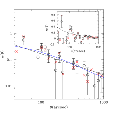
Figure 2: The two-point angular correlation function for the soft (open points) and total (crosses) bands respectively. The dashed line represent the best-fit power law $w(\theta)=(\theta_{\circ}/\theta)^{0.8}$ for the soft (0.5-2)keV band (see parameters in Table 1), while the continuous line represents the best fit $\Lambda$CDM ($\Omega_{\Lambda}=0.7$ and $h=0.7$) model in the framework of Basilakos & Plionis (2001) biasing model. In the insert we present the measured correlation function in linear scaling.

Our results are higher than those of Vikhlinin et al. (1995) who derive the angular correlation function from ROSAT pointed observations which have a comparable effective flux limit with our XMM pointings. The above authors find an angular clustering length of $\theta_{o}\sim 10$ arcsec, which reduces to 4 arcsec after correction for the amplification bias. Comparison with the results of Basilakos et al. (2004) shows that the hard band sources are more strongly clustered, at least on angular projection, ($\theta_{\circ}^{\rm hard}\simeq 22\pm 9$ for $\gamma=1.8$) compared to the soft band sources.

4 The spatial correlation length of the XMM soft sources

4.1 Inverting Limber’s equation

The spatial correlation function can be modeled as (de Zotti et al. 1990)

$$\xi(r,z)=(r/r_{\circ})^{-\gamma}\times(1+z)^{-(3+\epsilon)}\;\;,$$ (5)

where $\epsilon$ parametrizes the type of clustering evolution. If $\epsilon=\gamma-3$ (ie., $\epsilon=-1.2$ for $\gamma=1.8$), the clustering is constant in comoving coordinates (comoving clustering), which means that the amplitude of the correlation function remains fixed with redshift in comoving coordinates as the galaxy pair expands together with the Universal expansion. Alternatively, in the $\epsilon=-3$ model the clustering is constant in physical coordinates, while $\epsilon=0$ reflects the stable clustering model (eg. de Zotti et al. 1990).

We can relate the amplitude $\theta_{\circ}$ in two dimensions to the corresponding three dimensional one, $r_{\circ}$, using Limber’s integral equation (cf. Peebles 1993). For example, in the case of a spatially flat Universe, Limber equation can be written as

$$w(\theta)=2\frac{\int_{0}^{\infty}\int_{0}^{\infty}x^{4}\phi^{2}(x)\xi(r,z){\rm d}x{\rm d}u}{[\int_{0}^{\infty}x^{2}\phi(x){\rm d}x]^{2}}\;\;,$$ (6)

where $\phi(x)$ is the selection function (the probability that a source at a distance $x$ is detected in the survey) and $x$ is the proper distance related to the redshift through

$$x(z)=\frac{c}{H_{\circ}}\int_{0}^{z}\frac{{\rm d}t}{E(t)}\;\;,$$ (7)

with

$$E(z)=[\Omega_{\rm m}(1+z)^{3}+\Omega_{\Lambda}]^{1/2}$$ (8)

(see Peebles 1993). The number of objects in the given survey with a solid angle $\Omega_{s}$ and within the shell $(z,z+{\rm d}z)$ is:

$$\frac{{\rm d}N}{{\rm d}z}=\Omega_{s}x^{2}\phi(x)\left(\frac{c}{H_{\circ}}\right)E^{-1}(z)\;\;.$$ (9)

Therefore, combining the above system of equations, the expression for $w(\theta)$ satisfies the form

$$w(\theta)=2\frac{H_{\circ}}{c}\int_{0}^{\infty}\left(\frac{1}{N}\frac{{\rm d}N}{{\rm d}z}\right)^{2}E(z){\rm d}z\int_{0}^{\infty}\xi(r,z){\rm d}u$$ (10)

Note that, the physical separation between two sources, separated by an angle $\theta$ considering the small angle approximation, is given by:

$$r\simeq\frac{1}{(1+z)}\left(u^{2}+x^{2}\theta^{2}\right)^{1/2}\;\;.$$ (11)

Using eq.(5) and eq.(10) we obtain:

$$\theta_{\circ}^{\gamma-1}=H_{\gamma}\left(\frac{r_{\circ}^{\gamma}H_{\circ}}{c}\right)\int_{0}^{\infty}\left(\frac{1}{N}\frac{{\rm d}N}{{\rm d}z}\right)^{2}\frac{E(z)(1+z)^{-3-\epsilon+\gamma}}{x^{\gamma-1}(z)}{\rm d}z\;,$$ (12)

where $H_{\gamma}=\Gamma(\frac{1}{2})\Gamma(\frac{\gamma-1}{2})/\Gamma(\frac{\gamma}{2})$.

In order to perform the inversion we still need to determine the source redshift distribution ${\rm d}N/{\rm d}z$. Since we have no unbiased redshift information for our sources we can resort to a measure of ${\rm d}N/{\rm d}z$ using an estimate of their luminosity function. In flux-limited samples, there is a degradation of sampling as a function of distance from the observer (codified by the so called selection function). The latter also depends on the evolution of the source luminosity function but it is independent of the cosmological model, used in the derivation of the luminosity function. Thus for our X-ray sources the selection function can be written as:

$$\phi(x)=\int_{L_{\rm min}(z)}^{\infty}\Phi(L_{x},z){\rm d}L\;\;,$$ (13)

where $\Phi(L_{x},z)$ is their redshift dependent luminosity function. In this work we used the soft band luminosity functions of Miyaji, Hasinger & Schmidt (2000) and of Boyle et al. (1993). We also use different models for the evolution of the soft X-ray sources: a pure luminosity evolution (PLE) or the more realistic luminosity dependent density evolution (LDDE; Miyaji et al 2000). In Fig. 3 we present the expected redshift distributions of the soft X-ray sources for three different luminosity functions and evolution models. The LDDE model predicts a redshift distribution shifted to much larger redshifts with a median redshift of $\bar{z}\simeq 1.2$ (see also Table 2) comparing with both the Boyle et al (1993) and Miyaji et al (2000) luminosity functions with pure luminosity evolution. It is very interesting that the source redshift distribution of the ROSAT Lochman Deep field (Schmidt et al. 1998), albeit having a flux limit slightly lower than of our survey, traces quite well the LDDE predictions (see histogram in Fig. 3), a fact that supports this luminosity function evolutionary model. To quantify this claim we have performed a $\chi^{2}$ test between the observed and theoretical redshift distributions and found that the probability of consistency is 0.45 ($\chi^{2}/{\rm df}=0.97$), $<10^{-6}$ ($\chi^{2}/{\rm df}=8.5$) and 0.04 ($\chi^{2}/{\rm df}=2.1$) for the LDDE, PLE (Miyaji) and the PLE (Boyle) models, respectively.

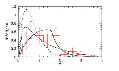
Figure 3: The redshift selection function for three different luminosity function models: (a) Miyaji et al (2000) with PLE (dashed line), (b) Miyaji et al (2000) with LDDE (continuous line) and (c) Boyle et al. (1993) with PLE (dot-dashed line). The histogram corresponds to the distribution of the Schmidt et al (1998) X-ray sources of the ROSAT Lochman Deep Field.

Table 2: The soft X-ray sources correlation length ($r_{\circ}$ in $h^{-1}$ Mpc) for different clustering models ($\epsilon$) and for the different luminosity functions and evolution models. The last column indicates the predicted median redshift, from the specific luminosity function used. The bold letters delineate the preferred cosmological model and the most updated luminosity function.

LF	Evol. Model	($\Omega_{m},\Omega_{\Lambda}$)	$r_{\circ}$ $(\epsilon=-1.2)$	$r_{\circ}$ $(\epsilon=-3)$	$\bar{z}$
Boyle	No evol.	(1,0)	7.9$\pm 0.6$	5.4$\pm 0.4$	0.50
Miyaji	No evol.	(1,0)	6.5$\pm 0.5$	4.9$\pm 0.4$	0.37
Boyle	PLE	(1,0)	12.0$\pm 1.0$	6.3 $\pm 0.5$	0.92
Miyaji	PLE	(1,0)	8.8$\pm 0.7$	$5.7\pm 0.4$	0.58
Miyaji	LDDE	(0.3,0.7)	${\bf 16.4\pm 1.3}$	${\bf 7.5\pm 0.6}$	1.19
Miyaji	LDDE	(1,0)	$11.2\pm 0.9$	5.0 $\pm 0.4$	1.19

4.2 Results

Using eq.(12), the LDDE luminosity evolution model and $\epsilon=-1.2$ we find within the concordance cosmological model a soft band correlation length of $r_{\circ}\simeq 16.4\pm 1.3\;h^{-1}$ Mpc. This value is comparable to that of Extremely Red Objects (EROs), luminous radio sources (Roche, Dunlop & Almaini 2003; Overzier et al. 2003; Röttgering et al. 2003) and hard X-ray sources (Basilakos et al. 2004) which are found to be in the range $r_{\circ}\simeq 12-19\;h^{-1}$ Mpc. It is interesting to mention that also radio sources which contain an AGN show strong clustering ($r_{\circ}\simeq 11\;h^{-1}$ Mpc), while the opposite is true for the case of radio sources showing no AGN activity (Magliocchetti et al. 2004).

However, our previously derived $r_{\circ}$ value is significantly larger than those derived from optical AGN surveys: $r_{\circ}\simeq 5.4-8.6\;h^{-1}$ Mpc (Croom & Shanks 1996; La Franca et al. 1998; Akylas et al. 2000; Croom et al. 2002; Grazian et al. 2004) as well as from the recent X-ray selected sample of Mullis et al. (2004) who find $r_{\circ}\simeq 7.4$ $h^{-1}$ Mpc. We can push our inverted $r_{\circ}$ values to approximate closely the latter results only if we use the constant in physical coordinates clustering evolution model ($\epsilon=-3$), in which case we obtain $r_{\circ}\simeq 7.5\pm 0.6\;h^{-1}$ Mpc, which is in excellent agreement with the Mullis et al. (2004) results. Note that earlier ROSAT soft X-ray clustering results of Carrera et al (1998) found a weaker clustering, with their upper limit of the linear clustering evolution model being marginally consistent with our $\epsilon=-3$ results.

In Table 2, we list the values of the correlation length, $r_{\circ}$, resulting from Limber’s inversion for different luminosity function, evolution models as well as for different cosmological models. We can attempt to disentangle the different sources of the apparent $r_{\circ}$ differences. Firstly, comparing the LDDE model between the Einstein de Sitter and the concordance ($\Omega_{\rm m}=1-\Omega_{\Lambda}=0.3$) Cosmological models it becomes evident that the effect of moving from the former to the latter model increases by $\sim 50\%$ the value of $r_{\circ}$ (for both $\epsilon$ cases). Note also that within the EdS cosmological model moving from the LDDE to the PLE luminosity evolution models decreases the value of $r_{\circ}$ by $\sim 20\%$ for $\epsilon=-1.2$, while for the $\epsilon=-3$ case there is no significant difference between the two luminosity evolution models. Therefore, although we do not have the PLE luminosity model parameters for the concordance cosmological model we may expect similar changes as before, which implies that within this cosmological and luminosity evolution (PLE) models we would obtain $r_{\circ}\sim 12.5$ and 7 $h^{-1}$ Mpc for the $\epsilon=-1.2$ and $\epsilon=-3$ models, respectively.

Also note that the change of the luminosity function model and thus of the redshift selection function, is always accompanied by a change of the median redshift of the corresponding redshift distribution.

We can attempt to parametrize the different luminosity model effects on the determination of $r_{\circ}$ by investigating its dependence on the median redshift of the source distribution as well as on the cosmological model. To do so we use a parametrized, by the characteristic redshift $\bar{z}$, analytical selection function, given by Baugh (1996):

$$\frac{{\rm d}N}{{\rm d}z}\propto z^{2}{\rm exp}\left[-\left(\frac{z}{z_{c}}\right)^{3/2}\right]\;\;,$$ (14)

where $\bar{z}=\sqrt{2}z_{c}$ is the median redshift. Although this formula has been derived from the distribution of optical galaxies while the redshift distribution of X-ray sources maybe different we find that at least for the case of the Miyaji et al (2000) luminosity function provides absolutely consistent results. For example, inserting eq. (14) in eq. (12) with $\bar{z}\simeq 1.19$ and $\epsilon=-1.2$ we find for the LDDE model $r_{\circ}\simeq 16.3\pm 2.0\;h^{-1}$ Mpc and $r_{\circ}\simeq 11.0\pm 1.5\;h^{-1}$ Mpc for the concordance and Einstein de Sitter models, respectively, which are in excellent agreement with the direct LDDE results (see Table 2). Similar consistency is found also for the other models presented in Table 2 (except for the models based on Boyle’s luminosity function which is due to their significant contributions from very large redshifts). In Fig. 4, we show the dependence of the derived $r_{\circ}$ on the median redshift of the source distribution for the two different cosmologies and two clustering evolution models. We also plot our direct results (using the different Miyaji et al. luminosity function models that provide different ${\bar{z}}$) of Table 2. The excellent consistency is evident which makes us confident of our results.

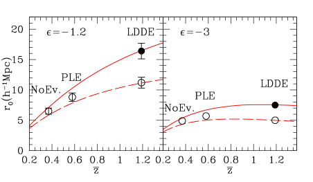
Figure 4: Comparison of the expected increase of $r_{\circ}$ as a function of the median redshift of the source redshift distribution for a concordance (continuous line) and an Einstein de Sitter model respectively, using the parametric selection function model of Baugh (1996). The results of Table 2 based on the Miyaji et al (2000) luminosity functions are plotted (filled circles for the concordance model and open for the Einstein de Sitter model).

Guided by Fig. 4 we can deduce that the PLE model of the Miyaji et al (2000) luminosity function would provide $r_{\circ}\simeq 12$ and 7 $h^{-1}$ Mpc within the concordance cosmological model for the $\epsilon=-1.2$ and $\epsilon=-3$ clustering models respectively.

5 The XMM sources cosmological bias

Within the framework of linear biasing (cf. Kaiser 1984; Benson et al. 2000), the mass-tracer and dark-matter spatial correlations, at some redshift $z$, are related by:

$$\xi(r,z)=\xi_{\rm DM}(r,z)b^{2}(z)\;\;,$$ (15)

where $b(z)$ is the bias evolution function.

We can quantify the evolution of clustering with epoch presenting the spatial correlation function of the mass $\xi_{\rm DM}(r,z)$ as the Fourier transform of the spatial power spectrum $P(k)$:

$$\xi_{\rm DM}(r,z)=(1+z)^{-(3+\epsilon)}\frac{1}{2\pi^{2}}\int_{0}^{\infty}k^{2}P(k)\frac{{\rm sin}(kr)}{kr}{\rm d}k\;,$$ (16)

where $k$ is the comoving wavenumber. Furthermore, the predicted spatial correlation function of the X-ray sources can be written as:

$$\xi(r,z)=\frac{R(z)}{2\pi^{2}}\int_{0}^{\infty}k^{2}P(k)\frac{{\rm sin}(kr)}{kr}{\rm d}k\;\;,$$ (17)

where

$$R(z)=(1+z)^{-(3+\epsilon)}b^{2}(z)\;\;\;.$$ (18)

As for the power spectrum of our CDM models, we use $P(k)\approx k^{n}T^{2}(k)$ with scale-invariant ($n=1$) primeval inflationary fluctuations and $T(k)$ the CDM transfer function. In particular, we use the transfer function parameterization as in Bardeen et al. (1986), with the corrections given approximately by Sugiyama (1995). Note that we also use the non-linear corrections introduced by Peacock & Dodds (1994).

5.1 Bias Evolution

The concept of biasing between different classes of extragalactic objects and the background matter distribution was put forward by Kaiser (1984) and Bardeen et al. (1986) in order to explain the higher amplitude of the 2-point correlation function of clusters of galaxies with respect to that of galaxies themselves.

The deterministic and linear nature of biasing has been challenged (cf. Bagla 1998; Dekel & Lahav 1999) and indeed on small scales ($r<10h^{-1}$Mpc) there are significant deviations from $b(r)=const$. Despite this, the linear biasing assumption is still a useful first order approximation which, due to its simplicity, it is used in most studies of large scale clustering (cf. Magliocchetti et al. 1999). In this paper however, we will work within the paradigm of linear and scale-independent bias. Based on different assumptions a number of bias evolution models have been proposed (eg. Nusser & Davis 1994; Fry 1996; Mo & White 1996; Matarrese et al. 1997; Tegmark & Peebles 1998; Bagla 1998; Plionis & Basilakos 2001). However, here we will discuss two that have been shown to describe relatively well the evolution even beyond $z\sim 1$.

• Merging Bias Model (hereafter B2): Mo & White (1996) have developed a model for the evolution of the the so-called correlation bias, using the Press-Schechter formalism. Utilizing a similar formalism, Matarrese et al. (1997) extended the Mo & White (1996) results to include the effects of different mass scales (see also Moscardini et al. 1998; Bagla 1998; Catelan et al. 1998; Magliocchetti et al. 2000). In this case we have that

  $$b_{\rm B2}(z)=0.41+\frac{(b_{\circ}-0.41)}{D^{\beta}(z)}\;\;\;,$$ (19)

  with $\beta\simeq 1.8$. Note that $D(z)$ is the linear growth rate of clustering (cf. Peebles 1993) scaled to unity at the present time.

• Bias from Linear Perturbation Theory (hereafter B3): Basilakos & Plionis (2001, 2003), using linear perturbation theory and the Friedmann-Lemaitre solutions of the cosmological field equations have derived analytically the functional form for the evolution of the linear bias factor, $b$, between the background matter and a mass-tracer fluctuation field. For the case of a spatially flat $\Lambda$ cosmological model ($\Omega_{\rm m}+\Omega_{\Lambda}=1$), the bias evolution can be written as:

  $$b_{\rm B3}(z)={\cal A}E(z)+{\cal C}E(z)K(z)+1$$ (20)

  with

  $$K(z)=\int_{1+z}^{\infty}\frac{y^{3}}{[\Omega_{\rm m}y^{3}+\Omega_{\Lambda}]^{3/2}}{\rm d}y$$ (21)

  or

  $$K(z)=(1+z)^{-1/2}F\left[\frac{1}{6},\frac{3}{2},\frac{7}{6},-\frac{\Omega_{\Lambda}}{\Omega_{\rm m}(1+z)^{3}}\right]$$ (22)

  where $F$ is the hyper-geometric function. Note that this approach gives a family of bias curves, due to the fact that it has two unknown parameters, (the integration constants ${\cal A},{\cal C}$). Basilakos & Plionis (2001, 2003) compared the B3 bias evolution model with other models as well as with the HDF (Hubble Deep Field) biasing results (Arnouts et al. 2002; Malioccietti 1999), and found a very good consistency. In this work, for simplicity, we fix the value of ${\cal C}$ being $\simeq 0.004$, as was determined in Basilakos & Plionis (2003) from the 2dF galaxy correlation function. It is evident that the bias factor at the present time can be obtained from eq.(20) for $z=0$

  $$b_{\rm B3}(0)={\cal A}+{\cal C}K(0)+1$$ (23)

  where we have used $E(0)=1$. Note that $K(0)\simeq 9.567$ for $\Omega_{\Lambda}=1-\Omega_{\rm m}=0.7$.

  

  Figure 5: The variation of $\Delta\chi^{2}$ around the best bias fit ($b_{\circ}$) using different clustering behaviours (left panel for $\epsilon=-1.2$ and right panel for $\epsilon=-3$). Note that the solid and dashed lines represent the bias from the linear perturbation (B3) and the merging (B2) bias models respectively.

  

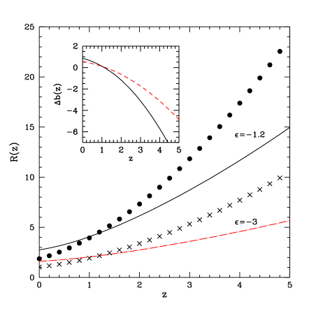
  Figure 6: The function $R(z)=(1+z)^{-(3+\epsilon)}b^{2}(z)$ as a function of redshift. The continuous line (B3 bias) and the filled point (B2 bias) types represent the $R(z)$ behaviour in the framework of a comoving clustering ($\epsilon=-1.2$), while the dot dashed line (B3 bias) and the crosses (B2 bias) are based on a clustering model which is constant in physical coordinates ($\epsilon=-3$). In the insert we present the difference, $\Delta b(z)=b_{\rm B3}(z)-b_{\rm B2}(z)$, between the (B3) and (B2) bias models as a function of $z$ for $\epsilon=-1.2$ (continuous line) and $\epsilon=-3$ (dashed line) respectively.

5.2 The bias at the present time $b_{\circ}$.

Based on the luminosity dependent density evolution (LDDE; Miyaji et al 2000) we quantify the bias factor at the present time $b_{\circ}$, performing a standard $\chi^{2}$ minimization procedure between the measured correlation function for the soft band (0.5-2)keV with that expected in our $\Lambda$CDM cosmological model,

$$\chi^{2}(b_{\circ})=\sum_{i=1}^{n}\left[\frac{w_{\rm XMM}(\theta^{i})-w_{\rm model}(\theta^{i},b_{\circ})}{\sigma^{i}}\right]^{2}\;\;.$$ (24)

where $\sigma^{i}$ is the observed $w(\theta)$ uncertainty.

In Fig. 5 we present for the two bias and clustering evolution models the variation of $\Delta\chi^{2}=\chi^{2}(b_{\circ})-\chi^{2}_{\rm min}(b_{\circ})$ around the best $b_{\circ}$ fit, while in Table 3 we list the results of the corresponding fits for all the considered models. The resulting present time bias is between: $b_{\circ}\simeq 1.05-1.90$ and $b_{\circ}\simeq 1.64-2.74$ for the B2 and B3 bias models, respectively. Note that the theoretical ($\Lambda$CDM $+$ B3 bias model) fit to the measured soft X-ray source angular correlation function is presented as the solid line in Fig.2.

Table 3: Results of the predicted soft X-ray sources bias. The correspondence of the columns is as follows: bias and clustering evolution models, $b_{\circ}$ is the bias at the present time, the reduced $\chi^{2}$ and the $\chi^{2}$ probabilities. Errors of the fitted parameters represent $1\sigma$ uncertainties.

Bias Model	$\epsilon$	$b_{\circ}$	$\chi^{2}/{\rm dof}$	$P_{\chi^{2}}$
B2	-1.2	$1.90\pm 0.10$	0.97	0.49
B3	-1.2	$2.74\pm 0.15$	0.86	0.60
B2	-3.0	$1.05\pm 0.05$	0.97	0.49
B3	-3.0	$1.64\pm 0.05$	0.84	0.63

In order to understand better the effects of AGN clustering, we present in Fig. 6 the quantity $R(z)$ (see eq.18) as a function of redshift for the concordance cosmological model and for different bias evolution models. It is quite obvious that the behaviour of the function $R(z)$ characterizes the clustering evolution with epoch; in general AGN clustering is a monotonically increasing function of redshift for both B2 and B3 biasing models. Figure 6, for example, clearly shows that the bias at high redshifts has different values in the different clustering models. In particular, for the comoving clustering, $\epsilon=-1.2$ (continuous line for B3 and filled points for B2), the distribution of soft X-ray sources is strongly biased ($1.90\raise-3.0pt\hbox{\hbox to0.0pt{\hbox{$\sim$}\hss}\raise 4.0pt\hbox{$<$}\ }b_{\circ}\raise-3.0pt\hbox{\hbox to0.0pt{\hbox{$\sim$}\hss}\raise 4.0pt\hbox{$<$}\ }2.74$), as opposed to the less biased distribution ($1.05\raise-3.0pt\hbox{\hbox to0.0pt{\hbox{$\sim$}\hss}\raise 4.0pt\hbox{$<$}\ }b_{\circ}\raise-3.0pt\hbox{\hbox to0.0pt{\hbox{$\sim$}\hss}\raise 4.0pt\hbox{$<$}\ }1.64$) in the $\epsilon=-3$ (dashed line for B3 and crosses for B2) clustering model. This is to be expected, simply because the value $\epsilon=-3$ removes the $(1+z)$ dependence from the $R(z)$ functional form and thus, produces a lower corresponding correlation length (see Table 2), in contrast with the comoving ($\epsilon=-1.2$) clustering case. In other words, the higher or lower correlation length corresponds to a higher or lower bias at the present time respectively, being consistent with the hierarchical clustering scenario (cf. Magliocchetti et al. 1999). Note, that the above predictions are in good agreement with those derived by Treyer et al. (1998), Carrera et al. (1998), Barcons et al. (2000) and Boughn & Crittenden (2004), who have found $b_{\circ}\sim 1-2$.

Regarding the predictions of the two bias models, we present in the insert of Fig. 6 the difference, $\Delta b(z)=b_{\rm B3}(z)-b_{\rm B2}(z)$, between the B3 bias model and the Mataresse et al. (1997) model B2 as a function of redshift. The B2 bias evolves significantly more than the B3 model at relatively low redshifts ($z\leq 1.0$), which could be attributed to our assumption that the galaxy number density is conserved in time. It is evident that merging processes, not taken into account in the B3 model, are probably important in the evolution of clustering.

It is evident that the behaviour of the inverted X-ray source spatial correlation function is sensitive to the different values of $\epsilon$ but there is also a strong dependence on the bias models that we have considered in our analysis.

We can attempt to select the most viable bias and the clustering evolution models by:

1. invoking the results of the local X-ray AGN clustering of Akylas et al (2000) and Mullis et al. (2004), who find $r_{\circ}\simeq 6.5$ and 7.4 $h^{-1}$ Mpc, respectively and

2. noting that the local galaxy distribution, with a correlation length $r_{\circ}\simeq 5\;h^{-1}$ Mpc, is unbiased with respect to the corresponding underline matter distribution (eg. Lahav et al. 2002; Verde et al. 2002).

These two facts leads us to a local bias between the X-ray selected AGN population and the underline matter distribution of:

$$b(0)=(r_{\circ,m}/r_{\circ,{\rm AGN}})^{-0.9}\sim(5/7)^{-0.9}\simeq 1.35\;,$$

which is consistent only with the $\epsilon=-3$ model of clustering evolution while it is in between the predictions of the two bias models used.

6 Conclusions

We have studied the angular clustering properties of the soft (0.5-e keV) X-ray point sources found in the XMM-Newton/2dF survey. We find that there is a strong ($3\sigma$) clustering signal. Indeed, if the two point angular correlation function is modeled as a power law, $w(\theta)=(\theta_{\circ}/\theta)^{0.8}$, then after correcting for the integral constraint and the amplification bias the best-fitting angular clustering length is $\theta_{\circ}\simeq 10.4\pm 1.9$ arcsec.

Inverting Limber’s equation and using the preferred luminosity dependent density evolution model for the luminosity function gives $r_{\circ}\simeq 16$ and 7.5 $h^{-1}$ Mpc, for the constant in comoving ($\epsilon=-1.2$) and in physical ($\epsilon=-3$) coordinates clustering evolution models, respectively. In the former case, the values for the clustering length are comparable with those of Extremely Red Objects (EROs) and luminous radio sources, and are significantly higher than those found from previous ROSAT surveys (e.g. Vikhlinin et al. 1995, Akylas et al. 2000, Carrera et al. 1998; Mullis et al. 2004) and optical QSO surveys such as the 2QZ (Croom et al. 2002) and that of Grazian et al. (2004). However, we obtain a quite good agreement with the above surveys, only in the latter case of a clustering evolution model where the clustering length remains constant in physical coordinates ($\epsilon=-3$).

Comparing the measured angular correlation function for the soft band (0.5-2)keV X-ray sources with the theoretical predictions of the preferred $\Lambda$CDM cosmological model ($\Omega_{\rm m}=1-\Omega_{\Lambda}=0.3$) and two bias evolution models, we find that the present bias values is in the range of $1.9\raise-3.0pt\hbox{\hbox to0.0pt{\hbox{$\sim$}\hss}\raise 4.0pt\hbox{$<$}\ }b_{\circ}\raise-3.0pt\hbox{\hbox to0.0pt{\hbox{$\sim$}\hss}\raise 4.0pt\hbox{$<$}\ }2.7$ for the $\epsilon=-1.2$ model and $1.0\raise-3.0pt\hbox{\hbox to0.0pt{\hbox{$\sim$}\hss}\raise 4.0pt\hbox{$<$}\ }b_{\circ}\raise-3.0pt\hbox{\hbox to0.0pt{\hbox{$\sim$}\hss}\raise 4.0pt\hbox{$<$}\ }1.6$ for the $\epsilon=-3$ model.

References

- [] Akylas, A., Georgantopoulos, I., Plionis, M., 2000, MNRAS, 318, 1036
- [] Arnouts, S., et al., 2002, MNRAS, 329, 355
- [] Bardeen, J.M., Bond, J.R., Kaiser, N. & Szalay, A.S., 1986, ApJ, 304, 15
- [] Bagla J. S. 1998, MNRAS, 417, 424
- [] Baldi, A., Molendi, S., Comastri, A., Fiore, F., Matt, G., Vignali, C., 2002, ApJ, 564, 190
- [] Barcons, X., &, Fabian, A. C., 1988, MNRAS, 230, 189
- [] Barcons, X., Carrera, F. J., Ceballos, M. T., Mateos, S., 2000, ’X-ray Astronomy 99: Stellar Endpoints, AGN and the Diffuse X-ray Background’, eds. White N. et al. AIP Conference Proceedings 599, p.3 (astro-ph/0001182)
- [] Basilakos, S., 2001, MNRAS, 3266, 203
- [] Basilakos, S. & Plionis, M., 2001, ApJ, 550, 522
- [] Basilakos, S. & Plionis, M., 2003, ApJ, 593, L61
- [] Basilakos, S., Georgakakis, A., Plionis, M., Georgantopoulos, I., 2004, ApJL, 607, L79
- [] Baugh C. M., 1996, MNRAS, 280, 267
- [] Benson A. J., Cole S., Frenk S. C., Baugh M. C., & Lacey G. C., 2000, MNRAS, 311, 793
- [] Boughn, S. P., Crittenden R. G., 2004, submitted, ApJ, astro-ph/0404348
- [] Boyle, B. J., & Mo, H. J., 1993, MNRAS, 260, 925
- [] Boyle, B. J., Griffiths, R. E., Shanks, T., Stewart, G. C., Georgantopoulos, I., 1993, MNRAS, 260, 49
- [] Búdavari, T., et al., 2003, ApJ, 595, 59
- [] Carrera, F. J., Barcons, X., Fabian, A. C., Hasinger, G., Mason, K. O., McMahon, R. G., Mittaz, J. P. D., Page, M. J., 1998, MNRAS, 299, 229
- [] Catelan, P., Lucchin, F., Mataresse, S. & Porciani, C., 1998, MNRAS, 297, 692
- [] Croom, S. M., & Shanks, T., 1996, MNRAS, 281, 893
- [] Croom, S. M., Boyle, B. J., Loaring, N. S., Miller, L., Outram, P. J., Shanks, T., Smith, R. J., 2002, MNRAS, 335, 459
- [] Davis, M., Efstathiou, G., Frenk, C. S., White, S.D.M.,1985, ApJ,292,371
- [] Dekel, A., & Lahav, O, 1999, ApJ, 520, 24
- [] de Zotti, G., Persic, M., Franceschini, A., Danese, L., Palumbo, G. G. C., Boldt, E. A., Marshall, F. E., 1990, ApJ, 351, 22
- [] Efstathiou, G., Bernstein, G., Katz, N., Tyson, J. A., Guhathakurta, P., 1991, ApJ, 380, L47
- [] Freedman, W., L., et al., 2001, ApJ, 553, 47
- [] Frenk, C.S., et al, 2000, astro-ph:0007362
- [] Fry J.N., 1996, ApJ, 461, 65
- [] Georgakakis, A., Georgantopoulos, I., Stewart, G. C., Shanks, T., Boyle, B. J., 2003, MNRAS, 344, 161
- [] Georgakakis, A., et al., 2004, MNRAS, 349, 135
- [] Georgantopoulos, I., Stewart, G. C., Shanks, T., Boyle, B J., Griffiths, R. E., 1996, MNRAS, 280, 276
- [] Grazian, A., Negrello, M., Moscardini, L., Cristiani, S., Haehnelt, M.G., Mataresse, S., Omizzolo, A., Vanella, E., 2004, AJ, 127, 592
- [] Hawkins, Ed, et al. 2003, MNRAS, 346, 78
- [] Kaiser N., 1984, ApJ, 284, L9
- [] Kirkman, D., Tytler, D., Suzuki, N., O’Meara, J.M., Lubin, D., 2003, ApJS, 149, 1
- [] La Franca F., Andreani, P., Cristiani, S., 1998, ApJ, 497, 529
- [] Lahav, O. et al., 2002, MNRAS, 333, 961
- [] Magliocchetti, M., Maddox, S. J., Lahav, O., Wall, J. V., 1999, MNRAS, 306, 943
- [] Magliocchetti, M., et al., 2004, MNRAS, 350, 148
- [] Mason, K. O., et al., 2000, MNRAS, 311, 456
- [] Matarrese S., Coles P., Lucchin F., Moscardini L., 1997, MNRAS, 286, 115
- [] Miyaji, T., Hasinger, G., Schmidt, M., 2000, A&A, 353, 25
- [] Mo, H.J, & White, S.D.M 1996, MNRAS, 282, 347
- [] Moscardini, L., Coles, P., Lucchin, F., Matarrese, S., 1998, MNRAS, 299, 95
- [] Mullis C. R., 2002, PASP, 114, 668
- [] Mullis C. R., Henry, J. P., Gioia I. M., Böhringer H., Briel, U. G., Voges, W., Huchra, J. P., 2004, ApJ, in press, astro-ph/0408304
- [] Nichol, R. C., Briel, O. G., Henry, P. J., 1994, ApJ, 267, 771
- [] Nusser & Davis, 1994, ApJ, 421, L1
- [] Olive, K.A., Steigman, G., Walker, T.P., 2000, Phys.Rep., 333, 389
- [] Overzier, R. A., Röttgering, H., Rengelink, R. B., Wilman, R. J. 2003, A&A, 405, 53
- [] Peacock, A. J., &, Dodds, S. J., 1994, MNRAS, 267, 1020
- [] Peebles, P.J.E., 1973, ApJ, 185, 413
- [] Peebles P.J.E., 1993. Principles of Physical Cosmology, Princeton University Press, Princeton New Jersey
- [] Peebles P.J.E., Ratra, B., 2003, RvMP, 75, 559
- [] Roche, N. D., Dunlop, J., Almaini, O., 2003, MNRAS, 346, 803
- [] Röttgering, H., Daddi, E., Overzier, R. A., Wilman, R. J. 2003, New Astronomy Reviews, 47, 309
- [] Schmidt, M. et al., 1998, A&A, 329, 495
- [] Shanks, T., & Boyle, B. J., 1994, MNRAS, 271, 753
- [] Soneira, R. M., &, Peebles, P. J. E., 1978, AJ, 83, 845
- [] Spergel, D. N., et al., 2003, ApJs, 148, 175
- [] Sugiyama, N., 1995, ApJS, 100, 281
- [] Tegmark M. & Peebles P.J.E, 1998, ApJL, 500, L79
- [] Tegmark M., et al. , 2004, PhRvD, 69, 3501
- [] Treyer, M., Scharf, C., Lahav, O., Jahoda, K., Boldt, E., Piran, T., 1998, ApJ, 509, 531
- [] Verde, L., et al, 2002, MNRAS, 335, 432
- [] Vikhlinin, A. & Forman, W., 1995, ApJ, 455, 109
- [1] Woods, D. & Fahlman, G.G., 1997, ApJ, 490, 11
- [] Yang, Y., Mushotzky, R. F., Barger, A. J., Cowie, L. L., Sanders, D. B., Steffen, A. T., 2003, ApJ, 585, L85