Reflections on Reflexions: I. Light Echoes in Type Ia Supernovae

Abstract

In the last ten years, observational evidences about a possible connection between Type Ia Supernovae (SNe) properties and the environment where they explode have been steadily growing. In this paper I discuss, from a theoretical point of view but with an observer’s perspective, the usage of light echoes (LEs) to probe the CSM around SNe of Type Ia since, in principle, they give us a unique opportunity of getting a three-dimensional description of the SN environment. In turn, this can be used to check the often suggested association of some Ia’s with dusty/star forming regions, which would point to a young population for the progenitors. After giving a brief introduction to the LE phenomenon in single scattering approximation, I derive analytical and numerical solutions for the optical light and colour curves for a few simple dust geometries. A fully 3D multiple scattering treatment has also been implemented in a Monte Carlo code, which I have used to investigate the effects of multiple scattering. In particular, I have explored in detail the LE colour dependency from time and dust distribution, since this is a promising tool to determine the dust density and derive the effective presence of multiple scattering from the observed properties. Finally, again by means of Monte Carlo simulations, I have studied the effects of multiple scattering on the LE linear polarization, analyzing the dependencies from the dust parameters and geometry. Both the analytical formalism and MC codes described in this paper can be used for any LE for which the light curve of the central source is known.

1 Introduction

In the last few years the study of light echoes (hereafter LEs) in Supernovae (SNe) has become rather fashionable, since they provide a potential tool to perform a detailed tomography of the SN environment (see Sugerman 2003 and references therein) and, in turn, can give important insights into the progenitor’s nature, a matter which is still under debate. Due to the typical number density of dust particles which are responsible for the light scattering, LEs are expected to have an integrated brightness about ten magnitudes fainter than the SN at maximum. For this reason, a SN Ia in the Virgo cluster is supposed to produce, if any, an echo at a magnitude V$\sim$21.0. This has the simple consequence that it is much easier to observe such a phenomenon in a Ia than in any other SN type, due to its high intrinsic luminosity. As a matter of fact, only four cases are known: the SNe Ia 1991T (Schmidt et al. 1994, Sparks et al. 1999) and 1998bu (Cappellaro et al. 2001), and the type II SN1987A (Crotts, Kunkel & McCarthy 1989, Crotts & Kunkel 1991, Xu, Crotts & Kunkel 1994, Crotts, Kunkel & Heathcote 1995, Xu, Crotts & Kunkel 1995) and 1993J (Sugerman & Crotts 2002). As expected, the LE detections for the two core-collapse events occurred in nearby galaxies: LMC (d=50 Kpc) and M81 (d=3.6 Mpc) respectively. Now, while a dusty environment is expected for explosions arising in massive and short-lived progenitors, this is in principle not the case for the kind of stars which are commonly supposed to generate Ia events, i.e. old population and low mass. This is why the detection of substantial dust in the immediate surroundings of thermonuclear SNe, or at least in a fraction of them, would indicate a different scenario.

Actually, several authors have pointed out that the observed characteristics of Ia’s, such as intrinsic luminosity, colour, decline rate, expansion velocity and so on, appear to be related to the morphological type of the host galaxy (Filippenko 1989, Branch & van den Bergh 1993, van den Bergh & Pazder 1992; Hamuy et al. 1996, Hamuy et al. 2000; Howell 2001). Since these objects represent a fundamental tool in Cosmology (see for instance Leibundgut 2000), it is clear that a full understanding of the underlying physics is mandatory in order to exclude possible biases in the determination of cosmological parameters like $\Omega$ and $\Lambda$. In this framework, disentangling between possible Ia sub-classes is a fundamental step. In this respect, an important year in the SN history is 1991, when two extreme objects were discovered, i.e. SN1991T (Filippenko et al. 1992a) and SN1991bg (Filippenko et al. 1992b). The former was an intrinsically blue, slow declining and spectroscopically peculiar event, while the latter was intrinsically red, fast declining and also showing some spectral peculiarities. From that time on, several other objects sharing the characteristics of one or the other event were discovered, indicating that these deviations from the standard Ia were, after all, not so rare. Of course, one of the most important issues which was generated by the discovery of such theme variations concerned the explosion mechanism and, in turn, the progenitor’s nature.

The growing evidences produced by the observations in the last ten years have clearly demonstrated that the sub-luminous events (1991bg-like) are preferentially found in early type galaxies (E/S0), while the super-luminous ones (1991T-like) tend to occur in spirals (Sbc or later). This has an immediate consequence on the progenitors, in the sense that sub-luminous events appear to arise from an old population while super-luminous ones would rather occur in star-forming environments and therefore would be associated with a younger population. This important topic has been recently discussed in a work by Howell (2001), to which I refer the reader for a more detailed review. What is important to emphasize here is that 1991T-like events tend to be associated with young environments and are, therefore, the most promising candidates for the study of LEs. Or, in turn, if LEs are detected around such kind of SNe, this would strengthen their association with sites of relatively recent star formation.

The first case of LE in a Ia (1991T) seems to confirm this hypothesis, in the sense that the SN was over-luminous and the host galaxy (NGC4527) is an Sbc and also a liner. Slightly less convincing is the other known case (1998bu), since the galaxy (NGC3368) is both an Sbc and a liner, but the SN is not spectroscopically peculiar. The only characteristic in common with SN1991T is its decline rate $\Delta m_{15}$, which is lower than average, even though not so extreme as in the case of 1991T. Nevertheless, the HST observations by Garnavich et al. (2001)) show that a significant amount of dust must be present within 10pc from the SN. Of course no statistically significant conclusion can be drawn from such a small sample, which definitely needs to be enlarged. For this reason, during the past years, I have been looking for new cases, the most promising of which was represented by SN1998es in NGC 632. This SN, in fact, was classified as a 1991T-like by Jha et al. (1998), who also noticed that the parent galaxy was an S0, hosting a nuclear starburst (Pogge & Eskridge, 1993). Moreover, the SN was found to be projected very close to a star forming region and to be affected by a strong reddening, which all together made SN 1998es a very good candidate for a LE study.

While the present paper is devoted to the theoretical aspects of the LE phenomenon, in a forthcoming article (Patat et al. in preparation) we will be dealing with the application of these results to the known cases of SNe 1991T, 1998bu and the test case of SN 1998es. In the same work we will also present high resolution spectroscopy for the three events and other unpublished data relevant for the LE discussion.

The paper is organized as follows. After giving a general introduction to the LE phenomenon in single scattering approximation in Sec. 2, in Sec. 3 I derive analytical solutions for a thin perpendicular sheet and a spherical shell to illustrate the effects of forward scattering. In Sec. 4 I then present a numerical solution for a double exponential dust distribution, typical of a spiral galaxy. Single scattering approximation is refined in Sec. 5, where I introduce the attenuation and the concept of LE effective optical depth. The inclusion of multiple scattering is presented in Sec. 6, where I illustrate the implementation of a Monte Carlo (MC) code, whose results are shown and discussed in Sec. 7. The same code is then used to compute the LE spectrum (Sec. 8) and broad band $(B-V)$ colour (Sec. 9), which is compared with the results obtained with the single scattering plus attenuation approximation. The effects of a change in the dust mixture are described and discussed in Sec. 10. In Sec. 11 I introduce the concepts of MC polarization calculations, which I have used in a code to study the effects of multiple scattering, presented in the same Section. Finally, in Sec. 12 I give a closing discussion and in Sec. 13 I briefly summarize my results.

2 Single Scattering Approximation

Starting with the pioneering work by Couderc (1939), the problem has been addressed by several authors (see for example Dwek 1983, Chevalier 1986, Schaefer 1987, Emmering & Chevalier 1989, Sparks 1994, Xu, Crotts & Kunkel 1994, Sparks 1997 and Sugerman 2003), who have all adopted the single scattering approximation. The only exception is the work by Chevalier (1986), who has used a MC code to study the case of a spherically symmetric stellar wind with a $r^{-2}$ dust density law.

Given the number of existing publications on this topic, I will give here only a brief introduction to the LE phenomenon in the single scattering approximation, while I will focus on the analytical and numerical solutions which I shall use later on to test the MC code.

2.1 Integrated echo light curve

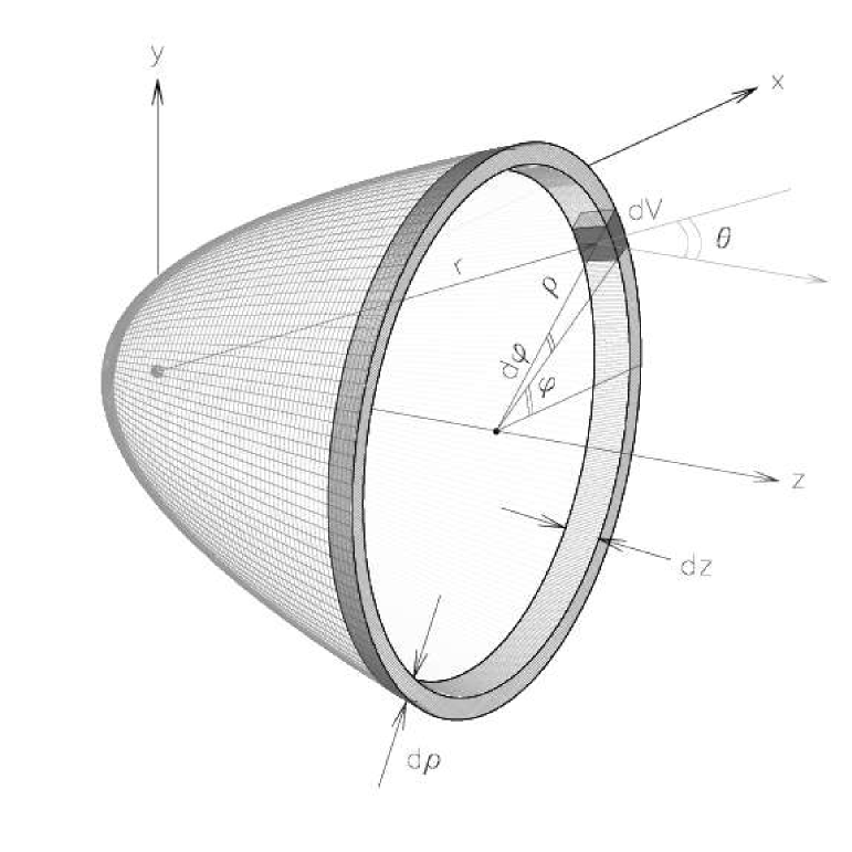
Figure 1: Geometry of the problem in single scattering approximation.

Let us imagine a SN immersed in a dusty medium at a distance $d$ from the observer. If we then consider the SN event as a radiation flash, whose duration $\Delta t_{SN}$ is so small that $c\;\Delta t_{SN}\ll d$, at any given time the LE generated by the SN light scattered into the line of sight and seen by the observer is confined in an ellipsoid, whose foci coincide with the observer and the SN itself. Since $d$ is supposed to be very large compared to all other geometrical distances, this ellipsoid can be very well approximated by a paraboloid, with the SN lying on its focus (see for example Chevalier 1986). More generally, the paraboloid can be regarded as the locus of those scattering elements which produce a constant delay $t$ and for this reason I will refer to it as the iso-delay surface. If $L(t)$ is the number of photons emitted per unit time by the source at a given wavelength, the flux of scattered photons per unit time and unit area which reach the observer at time $t$ is obtained integrating the flux scattered by the volume element $dV$ (see Fig. 1) over all iso-delay surfaces:

$$4\pi d^{2}\;F(t)=\int_{0}^{t}L(t-t^{\prime})\;f(t^{\prime})\;dt^{\prime}$$ (1)

The $f(t)$ function, which has the dimension of the inverse of a time, contains all the information about physical and geometrical properties of the dust and it is defined as follows:

$$f(t)=C_{ext}\;\omega\;\;c\int_{-ct/2}^{+\infty}\frac{\Phi(\theta)}{r}\int_{0}^{2\pi}n(\varphi,z,t)\;d\varphi\;dz$$ (2)

where $\varphi$ is defined as in Fig. 1, $r=z+ct$ is the distance of the volume element from the SN, $n=n(x,y,z)$ is the number density of scattering particles, $C_{ext}$ is the extinction cross-section, $\omega$ is the dust albedo, $\theta$ is the scattering angle defined by $\cos\theta=z/r$ and $\Phi(\theta)$ is the scattering phase function, normalized in order to have $\int_{4\pi}\Phi(\theta)d\Omega=1$. As usual in this kind of studies (cfr. Chevalier 1986), I have adopted the formulation proposed by Henyey & Greenstein (1941, hereafter H-G), which includes the degree of forward scattering through the parameter $g$: isotropic scattering is obtained for $g$=0 ($\Phi(\theta)=1/4\pi$) while $g$=1 gives a complete forward scattering. Both empirical estimates and numerical calculations for the optical wavelength range give $g\approx$0.6 (White, 1979), which corresponds to an average scattering angle $\overline{\theta}\sim$50^∘. More sophisticated calculations, including a full Mie’s treatment, show that the H-G formulation tends to underestimate the forward scattering, but the approximation is reasonably good (see for example Bianchi, Ferrara & Giovanardi 1996). As for the dust albedo, this is usually assumed to be $\omega\approx$0.6 (Mathis, Rumpl & Nordsiek, 1977).

From Eq. 1 it is clear that the out-coming scattered signal is the convolution of the SN signal $L(t)$ with the impulse response function $f(t)$ and therefore, at any given time $t$, the observer will receive a combined signal, which contains a sum of photons emitted by the SN in the whole time range $0-t$. This equation is formally identical to the one which describes the resulting acoustic wave reverberation in a given environment (see for example Spjut 2001).

The global flux received by the observer is obtained adding to the echo contribution the photons coming directly from the SN, after correcting for possible extinction:

$$F_{T}(t)=\frac{L(t)}{4\pi d^{2}}\;e^{-\tau_{d}}+F(t)$$ (3)

where

$$\tau_{d}=\int_{0}^{+\infty}C_{ext}\;n(0,0,z)\;dz$$ (4)

is the dust optical depth along the line of sight. Of course, if other dust is present but it does not contribute to the LE, because it is too far from the source, both the SN and the LE would suffer by additional extinction.

Due to the very short duration of the SN burst and in the single scattering approximation, there is a very good correspondence between the observed impact parameter $\rho=\sqrt{ct\;(2z+ct)}$ and the distance $r$ of the scattering material from the SN (see Fig. 1). This can be easily calculated as

$$r=\frac{1}{2}\;\left(\frac{\rho^{2}}{ct}+ct\right)$$ (5)

and it offers the unique possibility of measuring the third dimension of a resolved LE image with a spatial resolution of the order of $c\Delta t_{SN}$, provided that $d$ is known with some approximation. I note that this is always true, no matter what the dust geometry is, only provided that the dust optical depth is not too large to cause multiple scattering, which would introduce some degree of degeneracy in the $\rho$ vs. $r$ relation (see Sec. 7).

2.2 Echo surface brightness

If, for a given point $(x,y)$ on the sky plane, we consider the sum of all contributions along the $z$ axis, we can easily compute the echo surface brightness $\Sigma$ at any given time as:

$$\Sigma(x,y,t)=\frac{2c\;\omega\;C_{ext}}{4\pi d^{2}}\int_{0}^{t}\;\frac{L(t-t^{\prime})}{c^{2}t^{2}+\rho^{2}}\;n(x,y,t)\;\Phi(\theta)\;dt^{\prime}$$ (6)

The explicit dependency of $\Phi$ from $x,y$ and $t$ through the scattering angle $\theta$ can be obtained remembering that $\cos\theta=z/(z+ct)$ which, using the paraboloid equation (cfr. Chevalier 1986), can be reformulated as:

$$\cos\theta(\rho,t)=\left(\frac{\rho^{2}}{c^{2}t^{2}}-1\right)\left(\frac{\rho^{2}}{c^{2}t^{2}}+1\right)^{-1}$$ (7)

3 Simple analytical solutions

Eqs. 2 and 1 can be solved numerically, using the observed light curve of a typical Ia for $L(t)$. Nevertheless, instructive results can be obtained analytically if one assumes that the SN light curve is a flash:

$$L(t)=\left\{\begin{array}[]{ll}L_{0}&\mbox{for $t\leq\Delta t_{SN}$}\\ 0&\mbox{for $t>\Delta t_{SN}$}\end{array}\right.$$ (8)

In this approximation and for $t\gg\Delta t_{SN}$, the convolution in Eq. 1 becomes trivial and gives:

$$4\pi d^{2}\;F(t)=L_{0}\;\Delta t_{SN}\;f(t)$$ (9)

and hence the whole problem reduces to compute $f(t)$ defined by Eq. 2. The flash duration can be estimated from the observed light curve as $L_{0}\;\Delta t_{SN}=\int_{0}^{+\infty}L(t)\;dt$, and turns out to be of the order of 0.1 years for a typical Ia. The use of H-G formulation with $g\neq$0 in Eq. 2 makes the analytical integration possible only under certain conditions. For example, Chevalier (1986) has found an analytical solution for the case of a density law $n\propto r^{-2}$, typical of stellar winds. Here I will focus on two simpler cases only, those of a thin perpendicular sheet and a thin spherical shell, which are useful to illustrate the effect of forward scattering. In both geometries the solution becomes very easy, since $\mu$ can be considered constant along the iso-delay surfaces where $n\neq$0.

Let me first consider a thin sheet perpendicular to the line of sight, placed at a distance $R$ from the SN and with a thickness $\Delta R$. A limit on $\Delta R$ in order to fulfill the above condition can be derived differentiating the relation between $\mu$ and $z$ (see Sec. 2) and imposing $\Delta\mu\ll 1$. This gives:

$$\Delta R\ll\frac{(R+ct)^{2}}{ct}$$

Having this in mind and recalling that for $z=R$, one has that $\mu=z/r\equiv R/(R+ct)$, Eq. 2 can be integrated and it gives:

$$f(t)\simeq\frac{\omega\;C_{ext}\;c\;n_{0}\;(1-g^{2})}{2(1+g^{2}-2g\frac{R}{R+ct})^{3/2}}\;\ln\left(1+\frac{\Delta R}{R+ct}\right)$$ (10)

where, with the additional assumption that $\Delta R\ll R+ct$ (not necessarily included in the previous condition), the logarithmic term can be approximated with $\Delta R/(R+ct)$, as done by Cappellaro et al. (2001). As for the integrated luminosity, I notice that under these circumstances the time dependency is very mild. Therefore, using typical values for the relevant parameters ($g$=0.6, $\omega$=0.6, $\Delta t_{SN}$=0.1 yrs) and substituting Eq. 10 in Eq. 9, the normalized LE flux can be written as

$$4\pi d^{2}\;\frac{F(t)}{L_{0}}\approx 0.3\;\frac{\tau_{d}}{R}$$

where I have posed $\tau_{d}=C_{ext}\;n_{0}\;\Delta R$ (see Eq. 4). This basically means that, at least for a distant cloud ($R\gg ct$), the LE luminosity is inversely proportional to $R$ and directly proportional to $\tau_{d}$. For example, for a sheet placed at $R$=100 lyrs from the SN, in order to produce a LE 10 mags fainter than the SN at maximum, one needs an optical depth $\tau_{d}\simeq$0.03.

In general, the resulting echo will appear as a ring of radius $\rho_{R}=\sqrt{ct(2R+ct)}$ and thickness $\Delta\rho_{R}\simeq ct\;\Delta R/\rho_{R}$, with roughly constant surface brightness.

The overall effect of forward scattering can be evaluated directly from Eq. 10. In fact, for $R\gg ct$, it is $R/(R+ct)\simeq$1, so that the forward scattering term becomes approximately $(1+g)/(1-g)^{2}$. This means that going from $g=0$ to $g=0.6$, the echo maximum luminosity increases by more than a factor of 10. Moreover, as a consequence of the loss in the scattering efficiency due to the increase of the scattering angle with time, the resulting light curves get steeper. This is particularly true when the dust is not too far from the central source, while for increasing values of $R$ the time dependency of the forward scattering term tends to disappear (see Eq. 10).

The inclusion of forward scattering produces also a sensible flattening of the surface brightness profile. In fact, an increase of $g$ causes the material which is close to the SN to be less efficient in scattering the incoming photons, and this tends to balance with the fact that more distant material receives less photons from the SN but it is more effective in deflecting its light. Furthermore, for homogeneous distributions, the surface brightness at $\rho=ct$ decreases by a factor $(1-g^{2})/(1+g^{2})^{3/2}$ which, for $g=0.6$, corresponds to about one magnitude. This is relevant for the detection of the maximum polarization ring (see Sparks 1994 and the discussion in Sec. 11 here).

Another example of analytical solution in the case of $g\neq$0 is the one of a thin spherical shell of radius R and thickness $\Delta R\ll R$. In this case, since $R=z+ct$, we have that $\mu=(R-ct)/R$ and therefore the solution of Eq. 2 gives:

$$f(t)\simeq\frac{\omega\;C_{ext}\;c\;n_{0}\;(1-g^{2})}{2(1+g^{2}-2g\frac{R-ct}{R})^{3/2}}\;\ln\left(1+\frac{\Delta R}{R}\right)$$

Also in this case the LE would appear as a ring, whose radius $\rho_{R}=\sqrt{ct(2R-ct)}$ grows, reaches a maximum at $t=R/c$, decreases again and finally shrinks to zero for $t=2R/c$. As in the case of the thin sheet, the echo luminosity is approximately proportional to $\tau_{d}\;R^{-1}$ and forward scattering has a similar effect.

4 Numerical solution for a double exponential dust disk

The numerical integration of Eq. 2 allows one to solve the problem under the single scattering approximation for whichever dust geometry and input SN light curve.

For this purpose I have chosen to adopt a $V$ template light curve obtained smoothing the combined data sets of SNe 1994D (Patat et al. 1996, Richmond et al. 1995, Cappellaro et al. 1997) and 1992A (Suntzeff 1996, Cappellaro et al. 1997), two very similar and well sampled objects (see for example Patat et al. 1996). The result is shown in Fig. 2, where I have plotted the corresponding $(B-V)$ colour curve as well. The latter will serve to compare the intrinsic SN colour with that of the LE (see Sec. 9).

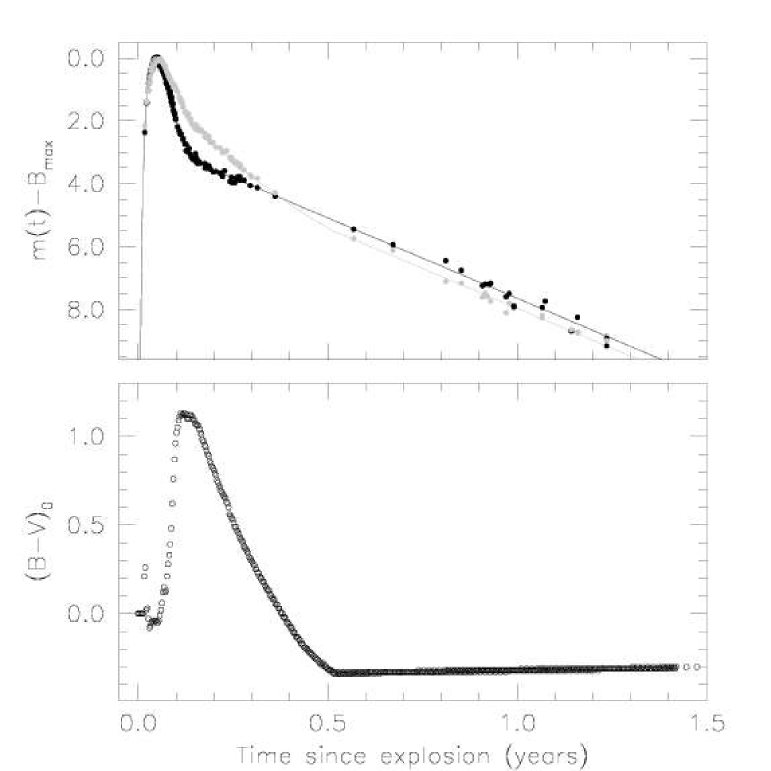
Figure 2: Template light curves for $B$ (black) and $V$ (gray) passbands. The solid lines trace the smoothed version used in the calculations while the filled dots indicate the observed data. The lower panel shows the corresponding $(B-V)$ colour curve.

In Fig. 3 I have traced the results obtained for a exponential face-on dust disk, whose density profile was modeled using the typical expression (see for example Bianchi, Ferrara & Giovanardi 1996):

$$n(R,Z)=n_{0}\;\exp\left(-\frac{R}{R_{d}}\right)\;\exp\left(-\frac{|Z|}{Z_{d}}\right)$$

where $R,Z$ are the cylindric galactic coordinates and $R_{d},Z_{d}$ are the characteristic radial and vertical scales. Following Bianchi et al. (1996), I have adopted $R_{d}$=4.0 kpc and $Z_{d}$=0.14 kpc, which can be considered as typical values for a spiral galaxy. The density $n_{0}$ is constrained by the central optical depth of the disk seen face-on, which is given by $\tau(0)=2n_{0}\;C_{ext}\;Z_{d}$. Imposing a typical value $\tau(0)$=1 (see Xilouris et al. 1999) and for $C_{ext}$= 5$\times$10²² cm², $n_{0}$ turns out to be 2.3 cm^-3. The SN was placed at $R_{SN}$=2$\times$10⁴ lyrs ($\sim$6 kpc) and $Z_{SN}$=300 lyr above the galactic plane, which imply an optical depth $\tau_{d}\approx$0.06.

For both isotropic and forward scattering I have run the calculations using a flash (dashed line) and the template $V$ light curve (thick solid line) and this shows that the results are pretty similar, except for the early phases, where the flash tends to produce a sharper and brighter peak. This is anyway irrelevant, since at such epochs the SN is typically more than 10 magnitudes brighter that the LE and therefore, at least for Ia’s, Eq. 8 gives a fair description of the real light curve.

The effect of forward scattering is clearly illustrated in Fig. 3: with $g$=0.6 the light curve starts to deviate from the radioactive tail when the SN is about 1.5 mag brighter than with $g$=0. Moreover, forward scattering has an effect on the resulting slope for $t>$3 yrs, which is 0.1 and 0.05 mag yr^-1 in the two cases respectively.

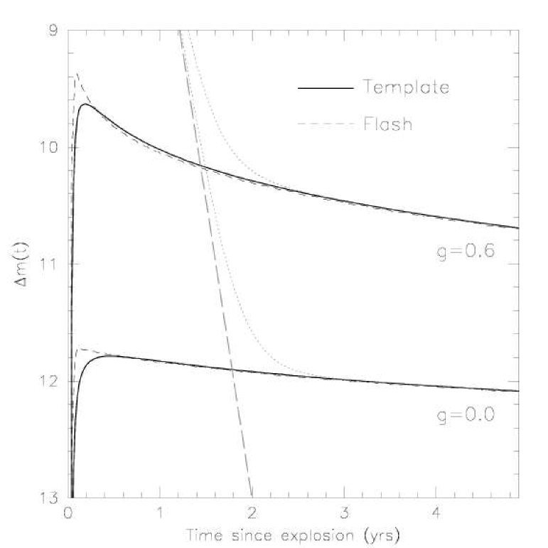
Figure 3: Single scattering numerical solutions for a face-on exponential disk for $g$=0 (lower curves) and $g$=0.6 (upper curves). The dotted curves trace the global light curves (SN+echo) while the long dashed line indicates the radioactive tail of the template light curve. In all examples $C_{ext}$=5$\times$10^-22 cm², $\omega$=0.6, $R_{SN}$=2$\times$10⁴ lyr and $Z_{SN}$=300 lyr were used (see text for more details).

In conclusion, under rather normal conditions, a Type Ia SN exploding in the disk of a spiral should always produce a LE which is of the order of 10 mag fainter than the SN at maximum, without the SN being heavily reddened. Of course, placing the SN in the inner parts of the disk or on the far side of the galaxy would increase the echo luminosity and the extinction suffered by the SN itself. For example, leaving all the other parameters unchanged and placing the SN at $Z_{SN}$=0 would enhance the LE by 0.7 mag, while the optical depth would grow to $\tau_{d}\sim$0.1, which is anyway still a rather low value. Since there are good reasons to believe that $1\leq\tau(0)\leq 5$ (Bianchi 2004), a Type Ia within 1-2 dust scale heights should always produce an observable LE, unless it is located very far from the galaxy center.

Using numerical integration, I have explored a few other simple cases, like front sheets with different inclinations, thin spherical shells, $r^{-2}$ winds and spherical clouds placed at different distances from the SN and with varying offsets with respect to the line of sight. In the latter case, when there is no scattering material along the line of sight, the LE starts to take place at $t>$0 and, in this respect, the parallel with acoustic physics becomes more pertinent, in the sense that the reflected signal starts to be detached from the direct impulse. Actually, in all cases where there is material on the line of sight, one should rather talk about light reverbs (LRs), which corresponds more appropriately to the analogous effect for acoustic waves.

In general, it turns out that all dust geometries produce similar LE luminosities and light curves. For typical values of $n_{0}$, $C_{ext}$, $\omega$ and $g$, the LE at three years after the explosion has an integrated brightness between 9 and 11 mag below SN maximum. Therefore, unless one is able to resolve the LE image, it is very difficult to disentangle between different dust geometries on the basis of the light curve shape alone.

5 Single scattering plus attenuation

The single scattering approximation can be refined in order to take into account the presence of absorption. Some times this is referred to as single scattering plus attenuation (hereafter SSA. See for example Wood et al. 1996). This approximation is obtained assuming that the fraction of a photon packet which reaches the observer has undergone one single scattering event on the iso-delay surface, while the remaining fraction was scattered by a number of interactions with the dust grains along the light path $l$ within the cloud system. The path length $l$ is defined as the cumulated distance traveled from the central source through the single scattering point and to the outer boundary of the dust cloud in the direction of the observer across regions with $n\neq 0$ (see Fig. 4). In the most general case, $l$ depends on the $\varphi,z,t$ coordinates of the scattering point (see Fig. 1 for the meaning of $\varphi$). The inclusion of attenuation is achieved introducing a $\exp{[-\tau_{a}(\varphi,z,t)]}$ factor in the definition of $f(t)$:

$$f(t)=C_{ext}\;\omega\;\;c\int_{-ct/2}^{+\infty}\frac{\Phi(\theta)}{r}\int_{0}^{2\pi}n(\varphi,z,t)\;e^{-\tau_{a}}\;d\varphi\;dz$$ (11)

where the attenuation optical depth $\tau_{a}$ is defined as

$$\tau_{a}(\varphi,z,t)=C_{ext}\;\int_{l}n(\mn@boldsymbol{l})\;|d\mn@boldsymbol{l}|$$ (12)

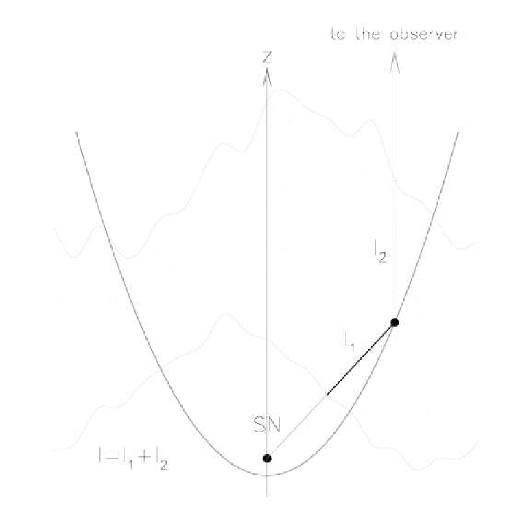
Figure 4: Meaning of the optical path $l$ in the single scattering plus attenuation approximation.

For one of the mean value theorems (see for example Råde & Westergreen 1999), one can also write:

$$f(t)=\frac{C_{ext}\;\omega\;c}{2}\;e^{-\tau_{eff}}\;G(t)$$ (13)

where:

$$e^{-\tau_{eff}}=\frac{\int_{-ct/2}^{+\infty}\int_{0}^{2\pi}\frac{\Phi(\theta)}{r}\;n(\varphi,z,t)\;e^{-\tau_{a}(\varphi,z,t)}\;d\varphi\;dz}{\int_{-ct/2}^{+\infty}\int_{0}^{2\pi}\frac{\Phi(\theta)}{r}\;n(\varphi,z,t)\;d\varphi\;dz}$$ (14)

and $G(t)$ is a time dependent function which includes the properties of dust and dust distribution. From Eq. 13 it is clear that, with the introduction of attenuation, the overall LE luminosity increases for growing density values until the optical depth reaches a critical limit. After that, self-absorption prevails and any further density enhancement causes the luminosity to decrease.

Table 1: Relevant parameters for the test-case geometries.

Geometry	$R$ $(R_{1})$	$\Delta R$ $(D,R_{2})$	$n_{0}(H)$
	lyrs	lyrs	cm-3
Sph. Shell	20	2	25, 125, 1000, 2500
Sph. Cloud	50	100	0.5, 2, 20, 50
Perp. Sheet	200	50	1, 5, 40, 100
$1/r^{2}$ Wind	0.5	7	110, 530, 4250, 10700

In general, $\tau_{eff}$ is time and geometry dependent and it can be regarded as a weighted optical depth for the LE at any given time. For example, it is easy to demonstrate that for a SN immersed in a perpendicular dust slab with uniform density, $\tau_{a}$ does not depend on $\varphi$ and $z$ coordinates, since $l=D+ct$. Therefore the solution of Eq. 14 becomes straightforward and it gives $\tau_{eff}=\tau_{d}+C_{ext}\;n_{0}\;ct$, which implies that the deviation from the single scattering approximation grows with time. A few more realistic examples of $\tau_{eff}$ calculations for the $V$ band are presented in Fig. 5, where I have considered four different geometries: a uniform spherical shell extended between $R$ and $R+\Delta R$, a distant perpendicular sheet placed at distance $D$ and with a thickness $\Delta R$, a distant spherical cloud with a radius $R$ and located at a distance $D$ in front of the SN and a spherically symmetric wind with $n(r)=n_{0}\;(R_{1}/r)^{2}$, which extends between $R_{1}$ and $R_{2}>R_{1}$. The first case can be considered as an approximation to the so-called contact discontinuity (see Sugerman 2003). This can be produced by the mass loss undergone by the Ia progenitor binary companion, through the interaction between the slow dense red supergiant wind and the fast blue supergiant wind (Emmering & Chevalier 1989). For the thin shell and perpendicular sheet I have adopted values which are very similar to those of Sugerman (2003; see his Table 4, second B case and first I case for SNe respectively), for the spherical cloud I have used a typical size of molecular clouds systems (see for example Mathis 2000), while for the stellar wind I have allowed for an inner dust-free cavity with radius $R_{1}$=0.5 lyrs ($\sim$5$\times$10¹⁷ cm, see for example Dwek 1983) and an outer radius $R_{2}/R_{1}$=15. As for the dust parameters, I have adopted the values reported by Weingartner & Draine (2001) and Draine (2003) for the $V$ passband (see also Table 2).

For all geometries, the number densities were set in order to produce the same optical depths $\tau_{d}$, i.e. the same SN extinction. The relevant parameters are summarized in Table 1. As one can notice, for the stellar wind case the higher optical depths imply dust densities which are rather unrealistic for this geometry and were included for completeness, also following Chevalier (1986).

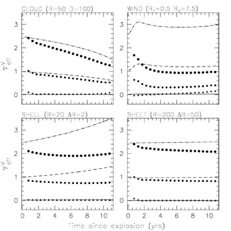
Figure 5: Example $\tau_{eff}$ calculations for $\tau_{d}$=0.03 (solid line), 1.0 (dashed line) and 2.5 (dashed-dotted line) in SSA approximation and $V$ passband. Geometrical parameters are indicated in each panel. For comparison, filled symbols trace the corresponding MC solutions (see Sec. 7).

As far as the relation between $\tau_{eff}$ and $\tau_{d}$ is concerned, it must be noticed that this depends very much on the dust geometry. For example, for a system with no dust along the line of sight, $\tau_{d}$=0, while $\tau_{eff}$ can assume any value. This clearly shows that, in general, the optical depth of a LE cannot be expressed in terms of the optical depth of the SN as seen from the observer. This is approximately true when the density is low or for some particular geometries only. For example, for the slab case seen before, $\tau_{eff}\simeq\tau_{d}$ for $ct\ll D$. As we will see, $\tau_{eff}$ actually depends not only on time and geometry, but also on the dust properties.

6 Monte Carlo simulations for multiple scattering

The idea behind Monte Carlo simulations is to follow each single photon packet along its random walk until it finally escapes the dust cloud. This procedure implicitly includes the treatment of multiple scattering and it is therefore suitable for all cases where the dust optical depth is large.

Following Chevalier (1986), here I will adopt the procedure outlined by Witt (1977), recalling the fundamentals of the method and describing in detail the aspects which are more specific to our case.

6.1 Isotropic and beamed emission

The whole process starts with the photon emission. Due to the dimensions of the dust clouds I am going to consider, I can assume that the SN is a point source lying at the origin of a coordinate system $x,y,z$. If $\Re_{i}$ is a random number uniformly generated in the range $0\leq\Re_{i}\leq 1$, the direction cosines are given by:

$$\begin{array}[]{lll}w_{0}&=&2\Re_{i}-1\\ u_{0}&=&\sqrt{1-w_{0}^{2}}\;\cos[\pi(2\Re_{i+1}-1)]\\ v_{0}&=&\sqrt{1-w_{0}^{2}}\;\sin[\pi(2\Re_{i+1}-1)]\end{array}$$

and obey to the usual condition $u_{0}^{2}+v_{0}^{2}+w_{0}^{2}$=1 (see Witt 1977, Eqs. 5, 6 and 7). When the scattering material, as seen from the central source, shows significant voids (like in the case of an isolated and distant cloud), the generation of random photons on the whole unit sphere would be not only a waste of computing time, but would also be inconsistent with the forced scattering technique, which I will introduce in the next sub-section. This problem can be solved emitting photons only within the solid angle $\Omega_{e}$ subtended by the cloud at the SN position. The fact that photons are artificially generated within a cone and not on the whole unit sphere is taken into account during the normalization of the light curve (see Sec. 6.4, Eq. 18).

6.2 Forced first scattering

To avoid wasting time with photons directly escaping the cloud, I have followed the common practice using the so called forced first scattering (Witt 1977). The basic idea behind this technique is to scatter each emitted photon, while the direct escape of non interacting photons is then taken into account using a weighting factor $W_{0}=1-\exp^{-\tau_{1}}$.

Once the random direction is generated, one needs to compute the total optical depth along the light path $\mn@boldsymbol{r}$:

$$\tau_{1}=\int_{0}^{r_{max}}n(\mn@boldsymbol{r})\;C_{ext}\;dr$$

where $r_{max}$ is the maximum dimension of the cloud or system of clouds along the emission direction. The next step is the random generation of $\tau\leq\tau_{1}$ at which the first scattering will occur. This is achieved using $e^{-\tau}$ as the probability density function, applying the inverse method and solving for $\tau$. This gives the following expression:

$$\tau=-\ln\left[1-\Re(1-e^{-\tau_{1}})\right]$$

which corresponds to Eq. 14 of Witt (1977), except from the fact that the latter has the incorrect sign.

Once this is done, one needs to determine the spatial position $\mn@boldsymbol{r}$ where the scattering occurs. For simple dust geometries this can be obtained inverting the analytical relation which links $\tau$ to the particle density function, while more general cases can be solved numerically (see for example Fischer, Henning & Yorke 1994), at the expense of computing time.

Irrespective of the adopted method, one has then to compute the photon direction after the scattering event, in order to be able to decide about its immediate destiny. For this purpose, as in the case of the analytical solutions, I have adopted the H-G scattering phase function. Again, using the inverse method, and solving for $\mu_{1}$ one finally obtains:

$$\mu_{1}=\frac{1}{2g}\left[(1+g^{2})-\frac{(1-g^{2})^{2}}{(1+2g\Re-g)^{2}}\right]$$ (15)

which corresponds to Eq. 19 of Witt (1977), except from the fact that the exponent 2 on the $(1-g^{2})$ term was lost. For $g=0$, Eq. 15 has to be replaced by $\mu_{1}=2\Re-1$.

Once $\mu_{1}$ is generated according to Eq. 15, the new direction cosines $(u_{1},v_{1},w_{1})$ need to be computed. This is done by the following coordinate transformation (see for example Bianchi, Ferrara & Giovanardi 1996, Appendix A4):

$$\begin{array}[]{l}u_{1}=u_{0}\cos\theta-\frac{v_{0}}{\sqrt{1-w_{0}^{2}}}\sin\theta\sin\phi\;+\frac{u_{0}w_{0}}{\sqrt{1-w_{0}^{2}}}\sin\theta\cos\phi\\ v_{1}=v_{0}\cos\theta-\frac{u_{0}}{\sqrt{1-w_{0}^{2}}}\sin\theta\sin\phi\;+\frac{v_{0}w_{0}}{\sqrt{1-w_{0}^{2}}}\sin\theta\cos\phi\\ w_{1}=w_{0}\cos\theta-\sqrt{1-w_{0}^{2}}\sin\theta\cos\phi\\ \end{array}$$

where $\theta$ is the scattering angle defined by $\mu_{1}=\cos\theta$, and $\phi$ is the scattering azimuth, from which I assume the scattering efficiency to be independent. This is generated simply as $\phi=\pi\;(2\Re-1)$, which gives a uniform distribution in the range $-\pi\leq\phi\leq\pi$.

6.3 Successive scatterings and final photon escape

The optical path to the next possible scattering can be computed with considerations which are similar to those I made for the first scattering, except from the fact that now photons are not forced to interact with the dust. Under this condition, the optical depth at which the next scattering event will occur is simply given by $\tau=-\ln\Re$. Whether the photon will escape or undergo further scatterings can be decided comparing $\tau$ with $\tau_{2}$, which is now computed along the scattered direction from the scattering point to $r_{max}$. If $\tau>\tau_{2}$ the photon will escape and, to compensate for the first forced scattering, a weight $W=\omega\;W_{0}$ will be given to it. The dust albedo $\omega<1$ accounts for the fact that during the scattering some photons can actually be absorbed.

In the case of $\tau\leq\tau_{2}$ the photon packet will be scattered again and hence the whole process has to be repeated, starting with the calculation of the scattering point, scattering direction and so on, until it finally escapes. In the general case of $N\geq 1$ scattering events, the final weight will be

$$W=\omega^{N}\;W_{0}$$ (16)

Once the emerging fraction of a given photon packet escapes, there are a series of parameters that are relevant for its temporal and spatial classification: a) the position $P_{N}(x_{N},y_{N},z_{N})$ of last scattering; b) the direction cosines after last scattering $(u_{N},v_{N},w_{N})$; c) the time delay accumulated by the scattered photons with respect to those which were emitted at the same time but traveled directly to the observer. All these numbers are needed to reconstruct integrated luminosity and surface brightness image (or profile) at a given time and from a given viewing direction.

While parameters a) and b) are immediately available, the calculation of time delay requires a little bit of more discussion.

6.4 Light curve reconstruction

Escaping photons can be seen only by an observer who lies on the line of sight coinciding with the last scattering direction $\mn@boldsymbol{p}(u_{N},v_{N},w_{N})$. If $\mn@boldsymbol{d}$ is the vector which goes from the coordinate system origin to the observer, $\mn@boldsymbol{r}(x_{N},y_{N},z_{N})$ defines the position of last scattering $P_{N}$ and $\mn@boldsymbol{l}=l\mn@boldsymbol{p}$ is the vector which goes from $P_{N}$ to the observer, one can clearly write $\mn@boldsymbol{d}=\mn@boldsymbol{r}+\mn@boldsymbol{l}$. Then if I set $k=\mn@boldsymbol{r}\circ\mn@boldsymbol{p}\equiv(x_{N}u_{N}+y_{N}v_{N}+z_{N}w_{N})$, I obtain $d^{2}=r^{2}+2kl+l^{2}$, which can be solved for $l$. One of the two solutions of this equation is not physical and therefore the light path from the last scattering to the observer is $l=-k+\sqrt{k^{2}+d^{2}-r^{2}}$, where $r^{2}=x_{N}^{2}+y_{N}^{2}+z_{N}^{2}$. For $d\gg r$ this gives $l\approx d-k$. Taking into account the random walk which was traveled before the last scattering, one finds that the total optical path is $L=l+\sum_{i=1}^{N}r_{i}$. Having this in mind, the arrival time $t_{a}$ can be easily computed as:

$$t_{a}=t_{e}+\sum_{i=1}^{N}\frac{r_{i}}{c}\;+\;\frac{l-d}{c}\simeq\sum_{i=1}^{N}\frac{r_{i}}{c}\;-\;\frac{k}{c}$$ (17)

where $t_{e}$ is the emission time. This has to be generated according to the input SN light curve $L(t)$, which in this case can be regarded as a probability density function. Applying the inverse method I can write:

$$\Re=\frac{1}{L_{0}\;\Delta t_{SN}}\int_{0}^{t_{e}}L(t)\;dt$$

Since, in principle, one does not have an analytical description of $L(t)$, the integral has to be evaluated numerically for a series of $t_{e}$ values and the result can be easily interpolated and inverted, so that entering the uniform random variable $\Re$ one gets $t_{e}$ with the correct distribution. Of course, in the case of flash approximation (see Eq. 8), the emission time is simply generated as $t_{e}=\Delta t_{SN}\;\Re$.

At this point, the light curve can be progressively computed just accumulating the weighted photon packets in time delay bins $\Delta T$ along a given direction and within a given solid angle $\Delta\Omega$. Now, if $\mn@boldsymbol{p}(u_{N},v_{N},w_{N})$ is the photon escaping direction and $\mn@boldsymbol{s}(s_{x},s_{y},s_{z})$ is the versor which identifies the line of sight, the angle $\psi$ formed by the two vectors is defined by $\cos\psi=\mn@boldsymbol{p}\circ\mn@boldsymbol{s}$. Photons are counted if $\cos\psi\geq$cos$\psi_{l}$, where the limiting angle can be defined as $\cos\psi_{l}=1-q$ and $\Delta\Omega=2\pi q$, with $0\leq q\leq 1$.

The bin size $\Delta T$, which in the end will give the time resolution, depends on the total number of generated packets and the signal-to-noise ratio one wants to achieve. The same applies to $\Delta\Omega$, which will govern the angular resolution.

Finally, in order to follow the same procedure I adopted for the analytical solutions, the resulting light curve needs to be normalized to the SN maximum light luminosity. This is achieved dividing it by the number of photons $F_{0}$ the observer would receive by the SN at maximum, within the solid angle $\Delta\Omega$ and in the time interval $\Delta T$, which is clearly given by

$$F_{0}=N_{phot}\;\frac{\Delta T}{\Delta t_{SN}}\;\frac{\Delta\Omega}{\Omega_{e}}$$ (18)

For spherically symmetric models, escaping photons can be both generated and collected all over the unit sphere ($\Delta\Omega=\Omega_{e}=4\pi)$, and hence the normalization is obtained dividing the photon counts by $N_{phot}\;\Delta T/\Delta t_{SN}$.

6.5 Echo surface brightness reconstruction

Escaping direction cosines and last scattering position can be used to derive the spatial energy distribution projected onto the plane perpendicular to the line of sight, which coincides with the plane of the sky. This can be achieved simply transforming the coordinates of the last scattering point $P_{N}(x_{N},y_{N},z_{N})$ in the new system $O(X,Y,Z)$, which is obtained rotating by an angle $\beta$ around the $z$-axis and by an angle $\gamma$ around the transformed $y$-axis. The rotation angles $\beta$ and $\gamma$ are defined by the escaping direction cosines as:

$$\begin{array}[]{ll}\sin\beta=v_{0}/\sqrt{1-w_{0}^{2}};&\cos\beta=u_{0}/\sqrt{1-w_{0}^{2}}\\ &\\ \sin\gamma=w_{0};&\cos\gamma=\sqrt{1-w_{0}^{2}}\end{array}$$ (19)

In this reference system, the plane of the sky coincides with the $Y,Z$ plane, while the $X$-axis coincides with the line of sight. The transformation equations are as follows:

$$\begin{array}[]{l}X=x_{N}\cos\alpha\cos\beta+y_{N}\sin\alpha\cos\beta+z_{N}\sin\beta\\ Y=-x_{N}\sin\beta+y_{N}\cos\beta\\ Z=-x_{N}\cos\beta\sin\gamma-y_{N}\sin\beta\sin\gamma+z_{N}\cos\gamma\end{array}$$

Of course, contrarily to what happens for the numerical integration of Eq. 6, MC simulations do not allow direct calculation of the echo surface brightness at a given time $t$, since the arrival times $t_{a}$ are scattered across the whole range allowed by the dust geometry. For this reason, one needs to perform a selection on the outcoming photons and collect them only if their arrival times satisfy the condition $t-\Delta T/2\leq t_{a}\leq t+\Delta T/2$. Due to the large difference between the overall echo duration and the time resolution $\Delta T$, this means that only a small fraction of the total number of generated photons will fall in the required time range.

In order to achieve a reasonable signal to noise ratio in the final results, this implies that a very large number (10${}^{8}-$10⁹) of photons must be generated.

7 Results of MC simulations

I have implemented the concepts discussed in the previous sections in a MC code, which I have used to study the effects of multiple scattering on the outcoming LEs for the four dust geometries described in Sec. 5. In all calculations I have adopted $C_{ext}$=5.21$\times$10^-22 cm², $g$=0.54 and $\omega$=0.66, which are typical of a canonical $R_{V}$=3.1 Milky Way mixture in the $V$ passband (see Draine 2003 and Sec. 8 here). For non spherically symmetric geometries, I have used $\Delta\Omega$= 2$\times$10${}^{-3}\pi$ ($q$=10^-3), which corresponds to a collecting beam with an angular semi-amplitude of $\sim$2.6 degrees.

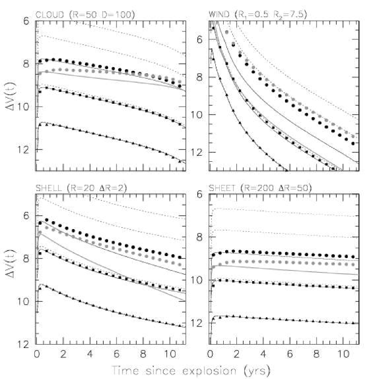
Figure 6: MC solutions for four different dust geometries for $\tau_{d}$=0.03 (triangles), 0.1 (squares), 1.0 (circles) and 2.5 (gray circles). For comparison, single scattering and SSA solutions are also indicated (dotted and solid lines respectively). For clarity, the SSA solution for $\tau_{d}$=2.5 has been traced with a thick gray line.

The basic effects of multiple scattering are illustrated in Fig. 6 for different values of $\tau_{d}$. While the MC simulated luminosity is only a few percents fainter than the single scattering solution in the low optical depth case ($\tau_{d}$=0.03), this difference becomes more and more marked as the dust density grows. For $\tau_{d}$=0.1 the deviation is $\sim$0.1 mag and it reaches about 1 mag for $\tau_{d}$=1.0. This is in very good agreement with the results found by Chevalier (1986) in the case of type II SNe surrounded by dust distributed with a $r^{-2}$ density law.

This is clearly due to the growth in the number of multiple scatterings. In fact, while the number of single scatterings tends to increase the echo luminosity, further scatterings contribute to the auto-absorption and therefore work against any brightness increase. As a consequence of these two competing mechanisms, the echo luminosity keeps growing for increasing values of $n$ until the fraction of photons which undergo pure single scatterings reaches 0.5. The scattered flux increases more and more slowly as the dust optical depth approaches some critical value ($\tau_{d}\simeq$1), after which the fraction of photons with $N_{scat}\geq 2$ becomes larger than 0.5 and the overall luminosity decreases for any further increase of $\tau_{d}$. The effect of a further dust density rise is illustrated by the gray circles, which were obtained for $\tau_{d}$=2.5. The exact details depend on the specific dust distribution but, for example, in the case of the thin shell, under these circumstances $N_{scat}$=1 in $\sim$15% of the cases only and this turns into an overall echo luminosity which is more than 1.5 mag fainter than the corresponding single scattering solution. Very similar results are obtained for the distant sheet and the $r^{-2}$ cases, while for the spherical cloud the behaviour is different, due to the fact that the intersection between the LE paraboloid and the cloud tends to rapidly decrease.

While this is not foreseen in the plain single scattering approximation, this is qualitatively predicted by the SSA approximation (solid curves), which gives reasonably good results for $\tau_{eff}<1$. In general, the simulations show that SSA successfully reproduces the early phases under a wide range of geometries, while it progressively deviates from the MC solutions as time goes by, and the deviation is larger for higher values of $\tau_{eff}$. The light curves produced by SSA are systematically fainter than multiple scattering solutions. This is a consequence of the assumption on which SSA is based, i.e. that attenuation acts as a pure absorption, which is approximately true at low optical depths only. In fact, when the density grows, photons which are deviated by the single scattering trajectory still have a probability of reaching the observer through further scatterings and can, therefore, contribute to the LE at later times. This effect, already noticed by Chevalier (1986), translates into a light curve flattening and it can be seen as the consequence of an increased average time delay accumulated by photons. The net effect is to reduce the effective LE optical depth with respect to $\tau_{eff}$ implied by the SSA approximation (see Fig. 5, filled symbols). The simulations show that this is more effective when the dust is confined closer to the SN and, for a given $\tau_{eff}$, when the dust density is higher.

More subtle is the outcome of multiple scattering on the radial surface brightness profile. For a uniform dust distribution, the simulations show that the resolved LE would always appear as a disk with a small surface brightness increase going outward and the gradient tends to become more pronounced for larger values of the dust optical depth. However, the effect is practically negligible.

Finally, the dust optical depth causes a progressive breaking of the relation between $r$ and $\rho$ expressed by Eq. 5 which, in principle, allows the direct calculation of the dust distance from the SN from the resolved LE image. In fact, in the high density regime the contribution by multiple scatterings tends to fill all the region internal to the iso-delay surface, mimicking the presence of dust close to the SN itself. I must notice, however, that the effect is not really pronounced and in most cases it would not be observable, the multiple scattering contribution being lost in the background noise.

8 Light echo spectrum

So far I have restricted the discussion to one single wavelength. But, in principle, a LE can be studied at any wavelength, provided that the dependencies of the relevant parameters, namely $C_{ext}$, $\omega$ and $g$, are known. If this is the case, the light echo spectrum can be computed using Eq. 1, where $L(t)$ is replaced by the spectrum $S(\lambda,t)$.

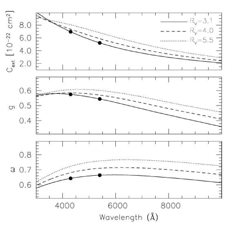
Figure 7: Behaviour of albedo (lower panel) forward scattering degree (middle panel) and extinction cross section (upper panel) for a Milky Way size dust distribution (Weingartner & Draine 2001, Draine 2003) and different values of $R_{V}$. Filled dots indicate the values at the effective wavelengths of $B$ and $V$ passbands.

For this purpose I have adopted the results published by Weingartner & Draine (2001) and Draine (2003) for a Milky Way mixture of carbonaceous and silicate grains with a canonical $R_{V}$=3.1. The behaviour of the relevant parameters in the optical spectral range is shown in Fig. 7 where, for comparison, I have also plotted the functions computed for higher values of $R_{V}$. As one can see, the dust albedo changes very little across the optical range (0.60$\leq\omega\leq$0.67), while the forward scattering degree shows a more significant variation. However, the strongest wavelength dependency is shown by the extinction cross-section whose behaviour, in the wavelength range 4000-9000 Å, is well approximated by a $\lambda^{-\alpha}$ law, with $\alpha$=1.35.

These functions were implemented in the codes by means of polynomial interpolations to the tabulated values.

8.1 Single scattering

In single scattering approximation, as in the case of the light curve, the echo spectrum  shape is independent of $n_{0}$, which governs the global luminosity only, while dust geometry and dust properties effects are included through the impulse response function $f(t)$. Now, the SN luminosity decays very fast and thus the bulk of optical radiation is emitted in a very short time range, which I will indicate as $\Delta t_{b}$. As a consequence, what really counts for the shape of the output spectrum observed at time $t$ is the behaviour of $f$ between $t-\Delta t_{b}$ and $t$. Therefore, the geometrical dependency is expected to be generally very mild at $t\gg\Delta t_{b}$. Exceptions to this might be encountered, for example, during the onset of a real echo, in which $f$ shows a pronounced transient phase. For the same reason, also variations on the forward scattering degree $g$ are expected to produce significant changes in the overall flux, but not in the spectral shape.

This is confirmed by the numerical solutions, for which I have used the spectroscopic data set of SN 1998aq (Branch et al., 2003). This includes 29 spectra obtained in the phase range $-$9${}^{d}\leq t\leq+$241^d and covers the wavelength range 3720-7160 Å. An example of LE spectrum is shown in Fig. 8: it is immediately clear that it does not resemble the SN spectrum at maximum, even if it has roughly the same colour (see also next section). For comparison, in Fig. 8 I have also plotted the time integrated spectrum of SN 1998aq (gray line). This is clearly redder than the actual LE spectrum, mainly due to the wavelength dependency of $C_{ext}$.

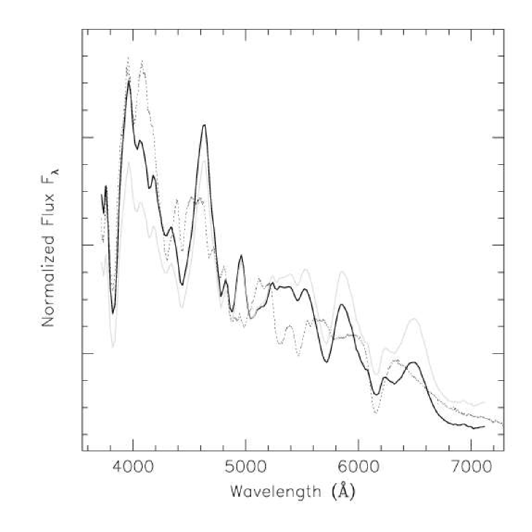
Figure 8: Light echo spectrum computed at $t$=2 yrs in single scattering approximation for a thin shell with $R$=20 lyr, $\Delta R$=2 lyr (black line) and $\tau_{d}\approx\tau_{eff}$=0.03 ($n_{0}$=25 cm^-2). For comparison, the solid gray line and the dotted line trace the time integrated spectrum and the maximum light spectrum of SN 1998aq (Branch et al. 2003), respectively. For presentation all spectra have been normalized to their integrated luminosity in the wavelength range 3720-7160 Å.

As I have already pointed out, in single scattering approximation an increase of the dust density produces a proportional increase in the overall echo flux, but no variation in its spectral appearance. In order to investigate optical depth effects, one in fact needs to use the multiple scattering approach. This is of course possible, even though the number of photons required to reach a reasonable signal to noise ratio in the output spectrum becomes very large. Practically this allows echo spectral synthesis in spherical symmetry only and, therefore, geometrical effects must be evaluated using broad band colours instead (see next section).

8.2 Multiple scattering

The procedure to compute a multiple scattering spectrum is identical to the one I have described for the light curve, with the exception that now the emission time $t_{e}$ and the emitted wavelength $\lambda_{e}$ have to be generated according to the input spectral distribution $S(\lambda,t)$. This can be easily achieved using the inverse theorem. Once the photon has completed its random walk through the dust, it is finally classified according to the arrival time $t_{a}$ and counted in the proper wavelength bin, whose amplitude $\Delta\lambda$ fixes the spectral resolution.

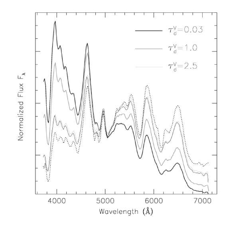
Figure 9: Synthetic LE spectra for a thin spherical shell ($R$=20 lyr, $\Delta R$=2 lyr) at $t$=2 yrs for increasing values of $\tau^{V}_{d}$ (dark to light thick lines). The thin line is the low optical depth spectrum reddened with a suitable extinction (see text); for clarity the spectrum was slightly shifted downward. For comparison, the dotted line traces a spectrum computed for $\tau^{V}_{d}$=2.5 with the SSA approximation. For presentation all spectra have been normalized to their integrated luminosity in the wavelength range 3720-7160 Å.

The results for a thin shell ($R$=20 lyr, $\Delta R$=2 lyr) and $t$=2 yrs are shown in Fig. 9, for three different values of $\tau_{d}$. As expected, the introduction of multiple scattering produces significant reddening in the spectrum. As a matter of fact, the spectra calculated for higher densities can be obtained directly from the one computed for the lowest $\tau_{d}$, applying the same wavelength dependency of $C_{ext}$ used for the LE calculation and a suitable optical depth $\tau_{eff}$. An example is presented in Fig. 9 (solid thin line), which was obtained using $\tau^{V}_{eff}$=1.95, i.e. the value derived from multiple scattering light curve model (see Fig. 5). For comparison, in Fig. 9 I have also plotted the spectrum obtained in SSA approximation for $\tau^{V}_{d}=2.5$ (dotted line). This appears to be too red with respect to the corresponding MC solution and the reason is that SSA tends to overestimate the LE optical depth by amounts which become larger at shorter wavelengths (see also next section).

9 Light echo colour

An alternative to spectral synthesis is the much less expensive calculation of broad band light curves, which can be combined to produce synthetic colours. In order to explore the potentialities of this method, I have studied the case of the $(B-V)$ colour, since for a Ia the LE is clearly brighter in these passbands than at redder wavelengths (see Fig. 8).

Table 2: Basic parameters for $B,V$ light curves and dust mixtures. Values for $C_{ext}$, $\omega$ and $g$ are from Weingartner & Draine (2001) and Draine (2003) for $R_{V}$=3.1 (first two rows) and $R_{V}$=5.5 (last two rows). Extinction cross section $C_{ext}$ is given per Hydrogen atom.

Passband	$\lambda$	$C_{ext}$	$\omega$	$g$	$\Delta t_{SN}$
	(Å)	(10-22cm2)			(yrs)
B	4300	6.95	0.64	0.57	0.0654
V	5400	5.21	0.66	0.54	0.0857
B		8.03	0.72	0.61
V		6.80	0.76	0.60

9.1 Single scattering plus attenuation

A first analytical estimate can be derived in SSA approximation, assuming that the input light curve is a flash. According to what I have shown in Secs. 2 and 5, under this assumption the echo flux at a given wavelength is $F=L_{0}\;n_{0}\;C_{ext}\;\Delta t_{SN}\;e^{-\tau_{eff}}\;G(t)$, where $G(t)$ is a time and wavelength dependent function related to geometry and dust properties. Applying this to the case of $B$ and $V$ passbands, and indicating with $(B-V)_{max}^{0}$ the unreddened colour of the SN at maximum, one can estimate the LE colour as:

$$(B-V) \approx (B-V)_{max}^{0}-2.5\;\log\;\frac{C_{ext}^{B}\;\omega^{B}\Delta t_{SN}^{B}}{C_{ext}^{V}\;\omega^{V}\;\Delta t_{SN}^{V}}$$ (20)

$$+ 1.086\;(\tau^{B}_{eff}-\tau^{V}_{eff})$$

where, due to the mild wavelength dependency of $g$ (see Table 2), I have assumed $G^{B}(t)\approx G^{V}(t)$. For low values of $\tau_{eff}$, after substituting the relevant parameters in Eq. 20, one gets $(B-V)\approx(B-V)_{max}^{0}\simeq-$0.1. Therefore, when the single scattering approximation is valid, the LE colour is roughly time and geometry independent. More generally, when the LE optical depth is not negligible, Eq. 20 implies that the resulting colour is reddened by auto-absorption ($\tau^{B}_{eff}>\tau^{V}_{eff}$). Moreover, it is directly related to the LE optical depth. In fact, using the values reported in Table 2, Eq. 20 can be rewritten as:

$$(B-V)\approx(B-V)_{max}^{0}+0.36\;\tau^{V}_{eff}$$ (21)

Thus, the observed $(B-V)$ colour can be used to estimate the effective optical depth of a LE, so that this is not a free parameter. Actually, numerical simulations show that the ratio $G^{B}(t)/G^{V}(t)$ can vary with time and geometries between 0.9 and 1.1, so that the previous simplified equation is expected to produce maximum errors of about $\pm$0.1 on the derived $(B-V)$ colour.

9.2 Multiple scattering

As we have seen in Sec. 7, when multiple scattering is at work, the echo luminosity does not scale linearly with the density and therefore the observed colour is expected to show a dependency on the dust optical depth. In particular, for increasing values of particle density, light curves appear to get fainter and fainter with respect to the corresponding single scattering solutions (see for example Fig. 6). Since this effect is supposed to get stronger for higher values of $C_{ext}$ (i.e. at shorter wavelengths), one expects the echo colour to become redder and redder as the density grows, as qualitatively foreseen also in the SSA approximation.

To explore these ideas in a more quantitative way, I have run a series of calculations using the parameters listed in Table 2, which were derived from the template light curves presented in Fig. 2 and from Draine’s models. The results for the thin shell and the $r^{-2}$ wind are shown in Fig. 10, for three different values of $\tau^{V}_{d}$, while Fig. 11 presents the cases of the distant sheet and the spherical cloud. For low optical depths the MC solutions are practically identical to the SSA solutions (solid and dashed curves) while, for larger densities, the calculated colour curves turn globally redder and redder for both geometries and progressively deviate from the SSA solutions. In general, these latter are systematically redder than the multiple scattering solutions and they give reasonable results only for $\tau_{eff}<$1.

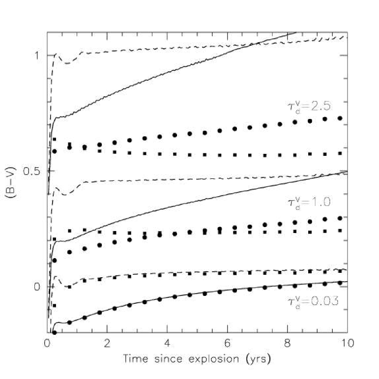
Figure 10: Multiple scattering $(B-V)$ colour curves for the thin shell (circles) and $r^{-2}$ wind (squares) for three different values of $\tau_{d}$. The corresponding SSA solutions are traced by solid and dashed curves respectively.

As far as the time dependence is concerned, the degree of forward scattering plays an important role. In fact, the random walk of a photon through the medium is influenced by the scattering phase function, in the sense that for high $g$ values, a photon tends to follow its emission direction, since small scattering angles are favored, and therefore its random walk will be shorter than for lower $g$ values. This means that the light curve is expected to declines faster at bluer wavelengths, where $g$ is higher (see Fig. 7). On the other hand, since $C_{ext}$ also increases bluewards, this produces the opposite effect, implying a light curve flattening, which is more efficient in the blue. As the simulations show, for the Milky Way mixture we have adopted (Weingartner & Draine 2001, Draine 2003) the two mechanisms tend almost to compensate each other, giving a rather flat time evolution, mostly driven by geometrical effects. As a matter of fact, the exact behaviour turns out to be pretty sensible to the wavelength dependency of $g$. Both SSA and MC calculation show that if one assumes $\partial g/\partial\lambda$=0, the $(B-V)$ colour tends to become bluer with time. Of course, the time evolution will also depend on the dust distribution, mainly through the allowed incoming angle range variation and the changes in $\tau_{eff}$. For example, when the dust is far from the SN, as in the case of the perpendicular sheet (Fig. 11, circles), this does not vary significantly with time, and therefore the colour curve is expected to be flatter than for dust close to the central source. This is also true for the distant spherical cloud (Fig. 11, squares), but the fact that $\tau_{eff}$ decreases as time goes by causes the LE to become progressively bluer.

The main conclusion is that the LE colour is practically time and geometry independent, especially after the initial onset phase ($t>$2 yrs), provided that the dust density is uniform. Therefore, any significant change in the observed colour has to be interpreted as a variation of $\tau_{eff}$ which, in turn, would signal the presence of density fluctuations.

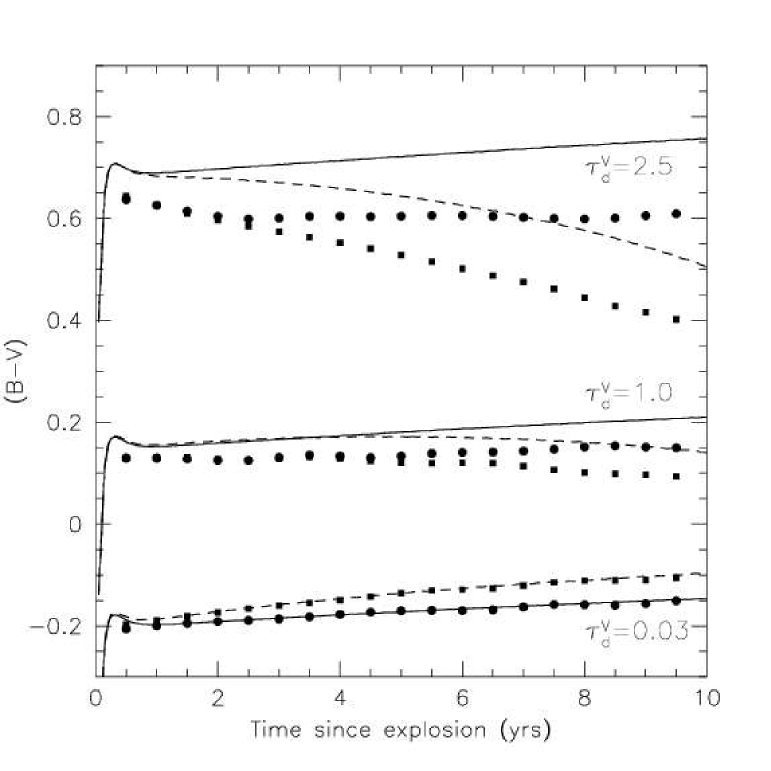
Figure 11: Multiple scattering $(B-V)$ colour curves for the perpendicular sheet (circles) and spherical cloud (squares) for three different values of $\tau_{d}$. The corresponding SSA solutions are traced by solid and dashed curves respectively.

As in the case of SSA approximation, one can use the approximate expression given by Eq. 21 to estimate the effective multiple scattering optical depth directly from the observed $(B-V)$ colour. It must be noticed that the assumption that $\tau^{B}_{eff}/\tau^{V}_{eff}\equiv C^{B}_{ext}/C^{V}_{ext}$, which holds in SSA approximation, is not strictly true when multiple scattering is at work. In general, in fact, this depends on the particular geometry and tends to be slightly larger than the cross sections ratio. Nevertheless, the simulations show that Eq. 21 gives reasonable results for $\tau^{V}_{eff}\leq 2$, where now $e^{-\tau_{eff}}$ is defined as the ratio between the multiple scattering solution and the corresponding single scattering solution.

10 Effects of a dust mixture change

In all calculations, I have so far adopted a canonical $R_{V}$=3.1 Milky Way dust composition. To illustrate the effects of a change in the dust mixture, I have run a series of calculations using Draine’s model corresponding to $R_{V}$=5.5. As shown in Fig. 7, the three dust parameters increase at all wavelengths. In the single scattering approximation, the consequences on $B$ and $V$ LE luminosities and colours can be anticipated from the following considerations. Neglecting the small variation in the forward scattering degree (see below), the LE luminosity is expected to change proportionally to $\omega\;C_{ext}$ (see Eq. 2). Using the suitable values (see Table 2) this turns into an increase of 0.29 and 0.44 mags in $B$ and $V$ respectively, while the $(B-V)$ colour becomes 0.15 mag redder.

When multiple scattering becomes important, the exact outcome is not so obvious. As I have shown in Sec. 7, a dust optical depth enhancement produces an increase in the LE luminosity until this reaches some maximum value, after which absorption prevails on scattering and the luminosity starts to decrease again. Therefore, increasing the scattering cross section causes an earlier luminosity saturation for any given dust density.

On the other hand, an albedo increase translates into smaller losses due to absorption, and therefore into a brighter light reverberation. The same mechanism tends also to delay the luminosity saturation, since higher values of the albedo turn into a smaller efficiency of multiple scattering in absorbing the radiation. The effect is going to be more pronounced at higher densities since, in those conditions, a fair fraction of the photon packets which reach the observer have undergone multiple scattering and therefore their weight, given by Eq. 16, strongly depends on the albedo. Finally, an higher forward scattering degree tends to increase the luminosity, especially at early phases, and to enhance the time dependency (see Sec. 3).

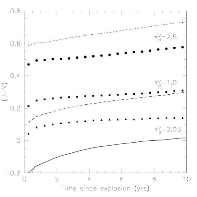
Figure 12: Multiple scattering $(B-V)$ colour curves for the thin shell case and for $R_{V}$=5.5 (symbols). The densities have been reduced in order to give the same optical depths $\tau_{d}^{V}$ as in Fig. 10. For comparison, the corresponding solutions for $R_{V}$=3.1 are also plotted (lines).

To illustrate the combined action of these mechanisms, in Fig. 12 I have plotted the comparison between the $(B-V)$ colours obtained for $R_{V}=3.1$ (lines) and $R_{V}=5.5$ (symbols), for the thin shell case ($R$=20 lyrs, $\Delta R$=2 lyrs). For the high $R_{V}$ solutions, the densities $n_{0}$ were adjusted in order to produce the same optical depths $\tau_{d}^{V}$, i.e. 0.03, 1.0 and 2.5. As expected, for the low density case, the $R_{V}$=5.5 solution (triangles) is about 0.15 mags redder than the $R_{V}$=3.3 one (solid line), the difference being larger at earlier phases due to the forward scattering effect. Then, at higher densities, the two solutions (squares and dashed line) become similar, implying that the optical depth effect is weakened by the albedo effect. Finally, for $\tau_{d}^{V}$=2.5 (circles and dotted line) the $R_{V}$=5.5 solution is bluer than the $R_{V}$=3.1 one. As a consequence, it is not possible to deduce the optical depth and the extinction law from the observed LE spectrum, even in the hypothesis the unreddened SN spectra are available. At least one of the two has to be assumed in order to derive the other. In fact, at least for the two different dust mixtures we have used here ($R_{V}$=3.1 and 5.5), one can produce very similar results just using different values for the LE optical depth.

11 Light echo polarization

Due to dust scattering, resolved LEs are expected to show strong linear polarization, which should reach its maximum degree for the dust which produces a scattering angle $\theta$=$\pi/2$ (Sparks 1994, 1997). In single scattering approximation, this occurs for dust lying on the SN plane, at a distance $ct$ from the SN itself.

In this section, I want to address the effect of multiple scattering on the observed polarization. A similar problem, even though in rather different contexts, has been approached using MC techniques by several authors (see for example Höflich 1991, Fischer, Henning & Yorke 1994, Code & Whitney 1995, Wood et al. 1996, Bianchi et al. 1996), and here I basically follow the same procedure they have adopted.

The fundamental concepts are those exposed by Chandrasekhar (1950, Chap. I; hereafter C50). In this view, a photon packet is characterized by a Stokes vector $\mn@boldsymbol{S}=(I,Q,U,V)$, which at each scattering event undergoes a transformation described by the following equation (C50, Eq. 210):

$$\mn@boldsymbol{S}=\mn@boldsymbol{L}(\pi-i_{2})\cdot\mn@boldsymbol{R}\cdot\mn@boldsymbol{L}(-i_{1})\cdot\mn@boldsymbol{S_{0}}$$ (22)

where $\mn@boldsymbol{S_{0}}$ denotes the incoming Stokes vector, $\mn@boldsymbol{R}$ is the so-called scattering matrix and $\mn@boldsymbol{L}$ is a Mueller rotation matrix (see e.g. Tinbergen 1996, Chap. 4) which transforms the Stokes vector from one reference system to the other. Following C50, I use as reference plane that defined by the photon direction and the $z$-axis, so that the required transformations are a counter-clock rotation of amplitude $i_{1}$, to bring the Stokes components into the scattering plane, and a clockwise rotation of amplitude $\pi-i_{2}$ to recompute the Stokes components with the new reference plane (see Van De Hulst 1980).

The explicit terms for $\mn@boldsymbol{L}$ can be derived from C50, Eq. 186 (see for example Code & Whitney 1995, Eqs. 3), while approximate expressions for $\mn@boldsymbol{R}$ terms in the case of H-G phase function can be found in White (1979).

11.1 Single scattering polarization

The effect of a single scattering on an unpolarized photon packet ($Q_{0}=U_{0}=V_{0}=0$) emitted by the central source, can be immediately computed using the approximate expressions found by White (1979) and this gives

$$P_{l}=p_{l}\;\frac{1-\cos^{2}\theta}{1+\cos^{2}\theta}$$ (23)

where $p_{l}$, the peak linear polarization, is of the order of 0.5. This result, first applied to LEs by Sparks (1994, Eq. 10), implies that the polarization is maximum for $\theta$=$\pi/2$, i.e. on the SN plane.

As for the polarization angle, it is easy to verify that the scattering plane and the electric field are perpendicular. As pointed out by Sparks (1994), this implies that the polarization direction is, at any given position, tangent to the circle centered on the SN, and this can be used as a distinctive feature to identify a LE.

Using Eq. 7 in Eq. 23, one can easily compute the expected radial polarization profile (see Fig. 13, solid line), which can be used to compare with the multiple scattering solutions I am going to present in the next sub-section. I note that in single scattering approximation the polarization degree is independent from $n_{0}$, $g$, $C_{ext}$ and $\omega$.

11.2 Depolarizing effect of multiple scattering

The implementation of polarization calculations in a MC code is fairly simple and it does not differ substantially from the one I have used to compute the echo surface brightness. After generating an unpolarized photon packet, its polarization state is followed along its random walk through Eqs. 22. In order to take into account the forced nature of first scattering, the initial Stokes vector is set to $\mn@boldsymbol{S_{0}}=(W_{0},0,0,0)$, where $W_{0}=1-exp(-\tau_{1})$ (see Sec. 6.2).

As usual in MC methods (see Kattawar & Plass 1968), the post-scattering Stokes parameters are weighted by the distribution which they were sampled from, which in this case is $P_{1}$ itself, i.e. the H-G phase function. In our case, all $P_{i}$ ($i$=1,2,3,4) terms of the scattering matrix contain $P_{1}$ as multiplicative factor (see White 1979) and, therefore, this corresponds to setting $P_{1}$=1. Finally, in order to account for the albedo effect and to make the radiation transfer consistent with the one I have used for the luminosity calculations, one would need to normalize the new Stokes parameters so that

$$I=\omega\;I_{0}$$ (24)

as done, for example, by Fischer, Henning & Yorke (1994). Rigorously speaking, this is true for the first scattering only, i.e. when the incoming light is unpolarized. In fact, after the first scattering episode, the light acquires some polarization degree and the fraction absorbed by the next event does depend on the direction of the electric field with respect to the scattering plane, through the following relation

$$I=\omega\;[I_{0}-p_{l}\frac{1-\mu^{2}}{1+\mu^{2}}\;(c_{1}Q_{0}+s_{1}U_{0})]$$ (25)

which is, in general, different from Eq. 24. Depending on the scattering circumstances, this implies that the effective albedo can be higher or lower than $\omega$, making this inconsistent with Eq. 24, which I have de facto used in the luminosity calculations. However, the simulations show that this inconsistency applies to photon packets individually, while the global effect tends to cancel and the average intensity ratio $I/I_{0}$ coincides with $\omega$, which can be therefore regarded as the average dust albedo (or the albedo for unpolarized light). In my calculations I have used Eq. 25, even if the results are practically identical to those one obtains from Eq. 24.

The normalized Stokes components after each scattering are used as input for the next one, until the packet escapes the dust system at a given projected position on the sky plane.

Since each photon packet is completely independent from the others (i.e. there is no phase relation between them), the resulting Stokes parameters are additive (CH50). This means that the polarization state at any given projected position can be obtained simply adding the Stokes vectors of all photon packets escaping from that position along a given direction.

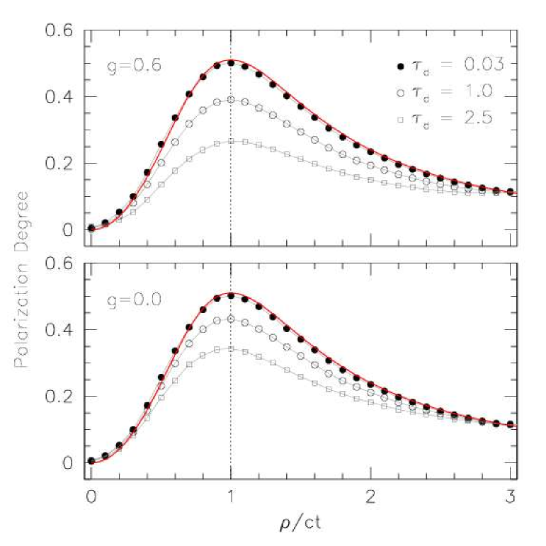
Figure 13: Radial polarization profiles for a homogeneous sphere ($R$=50 lyr) with forward ($g$=0.6, upper) and isotropic ($g$=0.0, lower) scattering, obtained for $t$=10 yrs.

In general, multiple scattering tends to act as a depolarizing mechanism (see for example Code & Whitney 1995 and Leroy 1998). In fact, successive scatterings occur with very different and stochastic angular parameters and it is very improbable that the polarization gained in the first scattering is increased. As a consequence, the maximum polarization ring is expected to become less and less marked, making its detection more and more difficult.

The results for a homogeneous sphere with $R$=50 lyr, which is intended to mimic the case of SN immersed in a homogeneous medium, are presented in Fig. 13 for different values for the density in the case of isotropic and forward scattering ($g$=0.6). The agreement with the analytical solution is very good for low optical depths. As anticipated, for increasing density values the polarization degree tends to decrease and the effect tends to be more pronounced for forward scattering.

It must be noticed that in all cases where the dust shows an axial symmetry around the line of sight, the net linear polarization one would measure in an unresolved LE image is null. Conversely, a net polarization degree significantly different from zero would signal the presence of asymmetry in the dust distribution, similarly to the case of an asymmetric SN envelope (see for example Höflich 1991). To illustrate this effect, I have calculated the net polarization one would observe from an unresolved uniform sphere placed at a distance $D$=$R$=50 lyr from the SN and seen with a viewing angle $\alpha$=0, $\pi/4$ and $\pi/2$, which turn out to be $<$0.1%, 0.8% and 6.0% respectively, for the usual values of relevant parameters ($n_{0}$=1 cm^-3, $\tau_{d}$=0.03, $g$=0.6, $\omega$=0.6). The observed polarization angle, defined as the direction of the electric field vibration, will then give an indication about the direction of maximum asymmetry, provided that linear polarization is significant with respect to the typical measurement errors.

Finally, after the second scattering, when the photon packets have acquired some degree of linear polarization, they may gain also some circular polarization. However, the simulations show that it is always $P_{c}<$5$\times$10^-4, which is within the noise of our calculations. Similar results were found by Code & Whitney (1995). For this reason circular polarization can be safely neglected (e.g. $V$=0).

12 Discussion

As I have shown, a LE with an optical luminosity $\sim$10 mag fainter than the SN at maximum can be produced by a Ia in the presence of dust with rather normal densities (1–10 cm^-3) and within 50–100 lyr (see Sec. 3). The resulting integrated light curves have typical slopes of 0.1–0.3 mag yr^-1. This becomes much higher if the dust is very close to the SN, as it is the case, for instance, of a stellar wind.

For a fixed distance between the SN and a given scattering element, the contribution to the total flux is not constant and it depends on its $z$ coordinate (see Fig. 1), due to the presence of forward scattering, which makes the process more efficient for foreground dust. Moreover, at any given time, the echo luminosity depends on the portion of the dusty region intersected by the iso-delay surface. For example, a spherical cloud placed in front of the SN at a distance $D$ along the $z$ axis is much more efficient than an identical cloud at the same distance $D$ but with its center located on the SN plane.

Of course, the two different geometries would produce very dissimilar echo resolved images, but in the lack of LE resolved images, it is very difficult to decode the dust geometry from the integrated light curve alone. In fact, unless the dust is confined within a region with a characteristic dimension $R<$ct, even very different geometries produce quite similar light curves (see Sec. 3).

The conclusion is that from the observed integrated light curve it is not possible to deduce the dust distribution, since the light curve shape is almost geometry independent and the echo luminosity can be tuned simply changing the dust density and its distance. Therefore, one is left with the question whether there are lots of dust far from the SN or a small amount of dust close to the SN.

One may argue that an increase in the dust optical depth would also produce observable reddening in the SN itself. This is true only under some particular conditions. For example, it could well be that there is a distant and optically thick cloud in front of the SN responsible for a significant reddening (but irrelevant for the light echo) while the scattering into the line of sight is produced by off-centered dust. A good example of such a case is given by SN 1989B, which was highly reddened but for which there is no clear LE detection (Milne & Wells 2002). As I will show in a forthcoming paper, where I will apply the results presented here to the known cases, SN 1998es had a similar behaviour. Due to the way the LE forms (Sec. 2), one can have in fact several possibilities and the LE detection can be accompanied by SN extinction or not, in the same way that a heavy SN reddening is not necessarily related to the actual onset of a LE.

As a matter of fact, LE properties depend on the global dust geometry, while the SN reddening is linked to the dust lying on the line of sight only. This is why $\tau_{d}$ and $\tau_{eff}$ have, in general, two different meanings, which tend to coincide only under special conditions. Therefore, unless one has LE resolved images and an estimate of the distance $d$ to the SN, the integrated light curve alone is not enough to answer our original question, i.e. whether the SN is close or far from a dusty region.

Fortunately, as we have seen, the inclusion of multiple scattering shows that the LE colour traces pretty well the effective dust optical depth (Sec. 7). So, if an observed colour including a reddening sensitive passband (i.e. blue) is available, one can draw some conclusions about the dust density and the importance of multiple scattering. In fact, for low dust optical depths ($\tau^{B}_{eff}\leq$0.3), the resulting $(B-V)$ colour is similar to the intrinsic colour of the SN at maximum light and it is practically independent from the geometry (Sec. 9.1). As a consequence, any redder observed colour would signal the presence of an higher optical depth. In turn, this would give an additional constraint when one tries to reproduce the observed echo luminosity, thus reducing the geometry/density degeneracy which, however, can be eliminated only when high resolution imaging is also available.

Under these favorable conditions one can hope to derive a 3D mapping of the SN surroundings, given the univocal relation between the distance $r$ of the scattering elements from the SN and their impact parameter $\rho$ (see Eq. 5).

It is true that, as MC simulations show, this relation tends to break down as the dust optical depth grows, since the phenomenon tends to acquire a non-local nature. The exact details depend on the dust geometry, but in general this takes place at pretty high values of $\tau_{eff}$. In this respect, the onset of multiple scattering is much more important for the resulting LE luminosity, which does not increase monotonically as the dust density grows (Sec. 7), a fact which is foreseen also in the single SSA approximation (Sec. 5). Since the effect is more pronounced at bluer wavelengths, this produces the colour effect I have just discussed. Speaking about this, it is worth noting that it is generally assumed that the LE has a colour similar to that of the SN at maximum light (corrected for reddening if there is any). As I have shown (Sec. 9), this is surely true when multiple scattering is negligible but, if the SN is surrounded by a dense dusty medium, both the SN and the echo are expected to be reddened, possibly by different amounts, since in general $\tau_{d}\neq\tau_{eff}$, so that one can have both an unreddened SN coupled to a red echo or a reddened SN associated with a blue echo. Both SNe 1991T (Schmidt et al. 1994) and 1998bu (Cappellaro et al. 2001) are examples of the latter instance. In fact, the integrated $(B-V)$ colour of the LE was about $-$0.1, while both SNe certainly suffered from significant extinction. The fact that the LEs are definitely blue seems to suggest that the SN reddening is generated by a front cloud whose characteristic dimension $R$ is smaller than $\sqrt{ct(2ct+D)}$ (where $D$ is the distance of the cloud from the SN itself), so that it does not contribute to the LE for $ct>-D+\sqrt{D^{2}+R^{2}}$, while the LE is generated by a less optically thick cloud. I will come back to this point in the forthcoming paper.

Besides the optical depth, which is directly related to $C_{ext}$ and plays a relevant role, dust albedo $\omega$ and forward scattering degree $g$ are also important. For this reason, the exact results for LE spectra and broad band colours depend on the dust mixture one adopts. As a first approximation, in my simulations I have used the canonical $R_{V}=3.1$ Milky Way composition Draine (2003). A possible further development of this work is the study of different dust composition effects, similarly to what has been done by Sugerman (2003).

Of course, the final results are expected to depend also on the SN light curve one adopts as input. All the simulations I have presented in this paper made use of a template Ia input light curve, derived from two normal events (e.g. SNe 1992A and 1994D). As I have shown (see Sec. 3), this can be very well approximated by a flash with a duration $\Delta t_{SN}$, a parameter which normally changes with wavelength (see also Table 2). One may wonder what happens if this parameter becomes larger, as it is the case for slow declining SNe like 1991T ($\Delta t_{SN}^{V}$=0.116 yrs). The answer is easy and it is given by Eq. 9, which was derived under simplifying assumptions: integrated LE luminosity is proportional to $\Delta t_{SN}$, and therefore slow declining events (e.g. 1991T-like) are expected to produce brighter echoes than fast decliners. The effect is mild, though, and the total range is of the order of 0.5 mag.

So far I have assumed that the distance $d$ to the SN is known, since the main purpose of our inquiry is to derive the dust geometry. But the paradigm can be in principle reversed, in the sense that the time evolution of a resolved LE can be used to infer the distance. This was attempted, for example, by Bond et al. (2003) and Tylenda (2003) for the case of V838 Mon, which has shown an impressive LE. This method, in principle promising because it gives a direct geometric distance measurement, has nevertheless a weak point. In fact, it requires the geometry to be known in order to properly use the apparent echo expansion to derive the distance (the discussion in Tylenda 2003). Different geometries can be of course disentangled looking at the expansion evolution, but this requires quite a long time baseline.

It must be noticed that this technique is applicable when the echo edges can be clearly detected and measured at different epochs, as in the case of V838 Mon, whose distance (6-8 kpc) makes this feasible, while for a SN at a typical distance of 15 Mpc this becomes practically not a viable method.

Another application of LEs for direct distance determination is the one suggested by Sparks (1994), which makes use of the strong polarization ring generated by the dust placed at a distance $ct$ from the SN on the $z$=0 plane (see Sec. 11). Provided that there is dust on the plane of the SN, this allows one to get distance estimates directly from polarimetric imaging. Since the maximum polarization ring obviously expands at the speed of light and not at the superluminal speed expected for the LE edges, this method is practically applicable to old SNe only ($t>$50 yrs), always provided that HST polarimetric data is available.

There are two problems that could hinder this technique. The first is that what counts for the polarization detection is the polarized flux which, if any, is smaller than the total flux. As I have shown, for a uniform dust distribution (which I have mimicked with a sphere centered on the SN) the total flux decreases at a rate of several tenths of a magnitude per year during the first years, just because of the efficiency loss due to forward scattering. This adds up to something of the order of several magnitudes in 50 years, making the detection of the polarized signal very difficult, even if its polarization degree remains constant. The effect is going to be worsened by the probable presence of a bright galaxy background, which would certainly introduce additional noise in the polarimetric measurements. Secondly, the presence of multiple scattering tends to depolarize the scattered light, again decreasing the chances of detection. Besides this, I should as well note that a poor imaging resolution tends to reduce the polarization one would actually measure (see for example Leroy 1998).

As I have mentioned, the full applicability of this method relies on the presence of dust on the SN plane. If this is not the case, for example because the region around the central source is empty within a radius larger than $ct$, one can obtain only a lower limit for the distance. An example of such a situation is given by V838 Mon (Bond et al. 2003). In general, even though the method is certainly promising and worthwhile of being pursued, I am persuaded that the use of LEs to study the SN environment is more rewarding than distance determination. After all, deriving the distance to the SN with a factor 2 precision is nowadays not a great progress, while the same accuracy on the estimate of the distance of a Ia from a molecular cloud would be of high interest, especially if this turns out to be small.

I like to conclude this discussion with the following consideration. I have mentioned several times that in pretty normal conditions, a Ia is expected to produce a LE about 10 magnitudes fainter than its luminosity at maximum. This is actually what happened for the two known cases of SNe 1991T (Schmidt et al. 1994) and 1998bu (Cappellaro et al. 2001) which, at around 2 years after the explosion, clearly deviated from the usual radioactive decay. As a matter of fact, as a result of a systematic LE search including 64 historical SNe, Boffi, Sparks & Macchetto (1999) have reported 16 possible candidates, only one of which is a genuine Ia, i.e. SN 1989B (but see also Milne & Wells 2002). Therefore, one may first inquire why only two events have been detected and immediately conclude that this is simply because in the vast majority of the cases there is not enough dust around Ia’s, not an unexpected conclusion for supposedly long-lived and small mass progenitors.

At least for resolved HST images, this point has been thoroughly addressed by Sugerman (2003) in his extensive work on the observability of LEs, and his conclusion is that many echoes were lost within the surface brightness fluctuations of background unresolved starlight. In the case of ground based observations, I must notice that there are only a few Ia’s observed at more than one year past maximum. In fact, this has always been a problem, both due to their faintness and to the presence of the host galaxy background. Therefore, it is difficult to give a final answer on the basis of the current list of LE detections and we will probably have to wait a bit more in order to have a statistically significant sample. This is even more true if only over-luminous SNe are associated with dusty regions.

What I can exclude here, at least on the basis of my calculations, is that very dense ($n_{0}>$30 cm^-3), very close ($r<$50 lyr) and very extended ($R>$30–50 lyr) clouds are not present in SNe of type Ia, for they would produce well observable LEs, which is seemingly not the case. Also, from the results shown in Sec. 4 for the double exponential galactic disk, it seems that Type Ia SNe tend to explode far from the host galaxy disk, at vertical distances from the galactic plane that are significantly larger than the dust height scale $Z_{d}$, otherwise they would produce, again, detectable LEs.

13 Conclusions

In this paper I have discussed the phenomenology of unresolved LEs, with particular attention to the effects of multiple scattering on integrated luminosity and broad band colours. Even if the treatment is absolutely general and it can be applied to LEs produced by any transient source, I have devoted my analysis to the SN Ia case, due to its relevance in the possible relation between the observed SN properties and the explosion environment. The main results I have obtained can be summarized as follows:

• A type Ia SN is expected to produce a LE $\sim$10 mag fainter than the SN at maximum when it is immersed in a medium with dust densities of the order of 1 cm^-3;

• If there is dust on the line of sight, the LE takes place immediately after the SN outburst, but it becomes visible only when the SN has faded away. This typically happens at 2-3 yrs past explosion;

• In those cases one should rather indicate the phenomenon as a light reverb to make the parallel with acoustic physics more pertinent;

• In general, the dust optical depth as seen from the SN along the line of sight, $\tau_{d}$, is not sufficient to describe the integrated LE properties. A better description is given by $\tau_{eff}$, which is a sort of weighted LE optical depth;

• The integrated LE light curve tends to decline with time, both due to geometrical effects and forward scattering. Higher forward scattering tends to produce faster declines;

• For typical values of the forward scattering degree ($g$=0.6) the decline rate during the first few years is of the order of 0.1$-$0.3 mag yrs^-1;

• It is not possible, on the basis of integrated LE curves alone, to deduce the dust geometry. This can be inferred only if LE resolved images are available;

• For low values of $\tau_{eff}$ ($\la$0.3) the LE phenomenon can be safely described with single scattering approximation.;

• For higher optical depths, auto-absorption becomes relevant and attenuation ($\tau_{eff}<$1) or, better, multiple scattering must be included;

• Multiple scattering has a number of effects, but the most important is the LE reddening, which does not strongly depend on the dust geometry;

• At low dust optical depths ($\tau_{eff}\la$0.3), the LE $(B-V)$ colour is similar to the intrinsic colour of the SN at maximum. The importance of multiple scattering can be judged on the basis of observed LE colors, which can give approximate values for $\tau_{eff}$;

• The LE spectrum is expected to change very slowly with time. It does not resemble any of the SN spectra, being a mixture of all SN spectra between $t$=0 and the time of observation;

• Being the product of scattering, a LE is expected to be highly polarized, with maximum polarization ($\sim$50%) at geometrical radius $ct$. Multiple scattering tends to act as a depolarizer, making the maximum polarization ring less and less pronounced;

• In general the polarized flux, which is what counts for the polarization detection, decreases with time. This hinders the application of polarimetric imaging for direct distance determination.

References

- Bianchi, Ferrara & Giovanardi (1996) Bianchi, S., Ferrara, A. & Giovanardi, C., 1996, ApJ, 465, 127
- Bianchi (2004) Bianchi, S., to appear in Astrophysics of Dust, ASP Conference series, A.N. Witt, Draine, B.T. & Clayton, G.C. eds.
- Branch & van den Bergh (1993) Branch, D. & van den Bergh, S., 1993, AJ, 105, 2231
- Branch et al. (2003) Branch, D., et al., 2003, AJ, 126, 1489
- Boffi, Sparks & Macchetto (1999) Boffi, F.R., Sparks, W.B. & Macchetto, F.D., 1999, A&As, 138, 253
- Bond et al. (2003) Bond, H.E., et al., 2003, Nature, 422, 405
- Cappellaro et al. (1997) Cappellaro, E., Mazzali, P.A., Benetti, S., Danziger, I.J., Turatto, M., Della Valle, M. & Patat, F., 1997, A&A, 328, 203
- Cappellaro et al. (2001) Cappellaro, E., et al., 2002, ApJ, 549, L215
- Chandrasekhar (1950) Chandrasekhar, S., 1950, Radiative Transfer, Oxford, Oxford Univ. Press
- Chevalier (1986) Chevalier, R., 1986, ApJ, 308, 225
- Code & Whitney (1995) Code, A.D. & Whitney, B.A., 1995, ApJ 441, 400
- Couderc (1939) Couderc, P. 1939, Ann. d’Astrophys., 2, 271
- Crotts, Kunkel & McCarthy (1989) Crotts, A.P.S., Kunkel, W.E. & McCarthy, P.J. 1989, ApJ, 347, L61
- Crotts & Kunkel (1991) Crotts, A.P.S. & Kunkel, W.E. 1991, ApJ, 366, L73
- Crotts, Kunkel & Heathcote (1995) Crotts, A.P.S., Kunkel, W.E. & Heathcote, S.R., 1995, ApJ, 438, 724
- Draine (2003) Draine, B. T., 2003, ApJ, 598, 1017
- Dwek (1983) Dwek, E. 1983, ApJ, 274, 175
- Emmering & Chevalier (1989) Emmering, R.T. & Chevalier, R.A., 1989, ApJ, 338, 388
- Fischer, Henning & Yorke (1994) Fischer, O., Henning, Th. & Yorke, H.W., 1994, A&A, 284, 187
- Filippenko (1989) Filippenko, A.V., 1989, PASP, 101, 588
- Filippenko et al. (1992a) Filippenko, A.V., et al., 1992a, ApJ, 384, L15
- Filippenko et al. (1992b) Filippenko, A.V., et al., 1992b, AJ, 104, 1453
- Garnavich et al. (2001) Garnavich, P. et al., 2001, AAS, 199, 4701G
- Hamuy et al. (1996) Hamuy, M., Phillips, M.M., Suntzeff, N.B., Schommer, R.A., Maza, J. & Aviles, R., 1996, AJ, 112, 2391
- Hamuy et al. (2000) Hamuy, M., Trager, S.C., Pinto, P.A., Phillips, M.M., Schommer, M.M., Ivanov, V. & Suntzeff, N.B., 2000, AJ, 120, 1479
- Henyey & Greenstein (1941) Henyey, L.C. & Greenstein, J.L., 1941, AJ, 93, 70
- Höflich (1991) Höflich, P., 1991, A&A, 246, 481
- Howell (2001) Howell, D.A., 2001, ApJ, 554, L193
- Jha et al. (1998) Jha, S., Garnavich, P., Challis, P. & Kirshner, R.P., 1998, IAU Circ. n. 7054
- Kattawar & Plass (1968) Kattawar, G.W. & Plass, G.N., 1968, App. Optics, 7, 1519
- Leibundgut (2000) Leibundgut, B., 2000, A&Ar, 10, 179
- Leroy (1998) Leroy, J.L., 1998, Polarization of light and astronomical observation, Gordon and Breach Science Publishers, p.31
- Mathis, Rumpl & Nordsiek (1977) Mathis, J.S., Rumpl, W. & Nordsiek, K.H., 1977, ApJ, 217, 425
- Mathis (2000) Mathis, J.S. 2000, in Allen’s Astrophysical Quantities, Cox, A. (Ed.), 4th ed., 2000, p. 523
- Milne & Wells (2002) Milne, P.A. & Wells, L.A., 2003, AJ, 125, 181
- Patat et al. (1996) Patat, F., Benetti, S., Cappellaro, E., Danziger, I.J., Della Valle, M., Mazzali, P.A. & Turatto, M., 1996, MNRAS 278, 111
- Pogge & Eskridge (1993) Pogge, R.W. & Eskridge, P.B., 1993, AJ, 106, 1405
- Råde & Westergreen (1999) Råde, L. & Westergreen, B., 1999, Mathematical Handbook for Science and Engineering, 4th Ed., Springer Verlag
- Richmond et al. (1995) Richmond, M.W. et al., 1995, AJ, 109, 2121
- Schaefer (1987) Schaefer, B., 1987, ApJ, 323, L47
- Schmidt et al. (1994) Schmidt, B.P., Kirshner, R.P., Leibundgut, B., Wells, L.A., Porter, A.C., Ruiz-Lapuente, P., Challis, P., & Filippenko, A.V., 1994, ApJ, 434, L19
- Sparks (1994) Sparks, W.B., 1994, ApJ, 433, 29
- Sparks (1997) Sparks, W.B., 1997, in The Extragalactic Distance Scale, Livio, Donhaue & Panagia eds., Cambridge University Press, Cambridge, p.281
- Sparks et al. (1999) Sparks, W.B., Macchetto, F., Panagia, N., Boffi, F.R., Branch, D., Hazen, M.L., & Della Valle, M., 1999, ApJ, 523, 585
- Spjut (2001) Spjut, E., 2001, in The Csound Book, R. Boulanger ed., MIT Press, Cambridge, p.507
- Sugerman & Crotts (2002) Sugerman, B.E.K. & Crotts, A.P.S., 2002, ApJ,581, L97
- Sugerman (2003) Sugerman, B.E.K., 2003, AJ, in press, astro-ph/0307245
- Suntzeff (1996) Suntzeff, N.B., 1996, in R. McCray and Z. Wang (eds.), Supernovae and Supernova Remnants, p.41, Cambridge University Press, Cambridge
- Tinbergen (1996) Tinbergen, J., 1996, Astronomical Polarimetry, Cambridge University Press, Cambridge, p.45
- Tylenda (2003) Tylenda, R., 2003, A&A, in press, astro-ph/0306555
- Van De Hulst (1980) Van De Hulst, H.C., 1980, Multiple Light Scattering, Tables, Formulas and Applications, Academic Press, Vol. 2, p.493
- van den Bergh & Pazder (1992) van den Bergh, S. & Pazder, J., 1992, ApJ, 390, 34
- Weingartner & Draine (2001) Weingartner, J.C. & Draine, B.T. 2001, ApJ, 548, 296
- White (1979) White, R.L., 1979, ApJ, 229, 954
- Witt (1977) Witt, A.N., 1977, ApJs, 35, 1
- Wood et al. (1996) Wood, K., Bjorkman, J.E., Whitney, B. & Code, A.D., 1996, ApJ, 461, 828
- Xilouris et al. (1999) Xilouris, E.M., Byun, Y.J., Kylafis, E.V., Paleologou, E.V. & Papamastorakis, J. 1999, A&A, 344, 868
- Xu, Crotts & Kunkel (1994) Xu, J., Crotts, A.P.S. & Kunkel, W.E., 1994, ApJ, 435, 274
- Xu, Crotts & Kunkel (1995) Xu, J., Crotts, A.P.S. & Kunkel, W.E., 1995, ApJ, 451, 806