Bunching Instability of Rotating Relativistic Electron Layers and Coherent Synchrotron Radiation

Abstract

We study the stability of a collisionless, relativistic, finite-strength, cylindrical layer of charged particles in free space by solving the linearized Vlasov-Maxwell equations and compute the power of the emitted electromagnetic waves. The layer is rotating in an external magnetic field parallel to the layer. This system is of interest to understanding the high brightness temperature of pulsars which cannot be explained by an incoherent radiation mechanism. Coherent synchrotron radiation has also been observed recently in bunch compressors used in particle accelerators. We consider equilibrium layers with a ‘thermal’ energy spread and therefore a non-zero radial thickness. The particles interact with their retarded electromagnetic self-fields. The effect of the betatron oscillations is retained. A short azimuthal wavelength instability is found which causes a modulation of the charge and current densities. The growth rate is found to be an increasing function of the azimuthal wavenumber, a decreasing function of the Lorentz factor, and proportional to the square root of the total number of electrons. We argue that the growth of the unstable perturbation saturates when the trapping frequency of electrons in the wave becomes comparable to the growth rate. Owing to this saturation we can predict the radiation spectrum for a given set of parameters. Our predicted brightness temperatures are proportional to the square of the number of particles and scale by the inverse five-third power of the azimuthal wavenumber which is in rough accord with the observed spectra of radio pulsars.

I Introduction

The high brightness temperatures of the radio emission of pulsars ($T_{B}\gg 10^{12}$K) implies a coherent emission mechanism (Gold, 1968, 1969; Goldreich & Keeley, 1971; Manchester & Taylor, 1977; Melrose, 1991) and some part of the radio emission of extragalactic jets may be coherent (Bisnovatyi-Kogan & Lovelace, 1995). Recently, coherent synchrotron radiation (CSR) has been observed in bunch compressors (Loos, 2002; Byrd, 2002; Kuske, 2003) which are a crucial part of future particle accelerators. When a relativistic beam of electrons interacts with its own synchrotron radiation the beam may become modulated. If the wavelength of the modulation is less than the wavelength of the emitted radiation, a linear instability may occur which leads to exponential growth of the modulation amplitude. The coherent synchrotron instability of relativistic electron rings and beams has been investigated theoretically by Goldreich & Keeley (1971); Heifets & Stupakov (2001); Stupakov & Heifets (2002); Heifets (2001); Byrd (2003). Goldreich and Keeley analyzed the stability of a ring of monoenergetic relativistic electrons which were assumed to move on a circle of fixed radius. Electrons of the ring gain or lose energy owing to the tangential electromagnetic force and at the same time generate the electromagnetic field. Uhm et al. (1985) analyzed the stability of a relativistic electron ring enclosed by a conducting beam pipe in an external betatron magnetic field. A distribution function with a spread in the canonical momentum was chosen for their analysis. For simplicity the effect of the betatron oscillations was not included in their treatment. They find a resistive wall instability and a negative mass instability. Furthermore, they find an instability which can perturb the surface of the beam. Heifets (2001) analyzed the stability of a ring of relativistic electrons in free space including a small energy spread which gives a range of radii such that particles on the inner orbits can pass particles on outer orbits. Byrd (2003) has developed a similar model which includes the effects of the conducting beam pipe. Numerical simulations by Venturini & Warnock (2002) show the burst-like nature of the coherent synchrotron radiation.

The present work analyzes the linear stability of a cylindrical, collisionless, relativistic electron (or positron) layer or E-layer (Christofilos, 1958). Particle densities in pulsar magnetospheres are very low, of order the Goldreich-Julian charge density $n_{GJ}={\bf\Omega\cdot B}/2\pi ce\sim 10^{11}s\,{\rm cm^{-3}}(B/10^{12}\,{\rm G})(R/r)^{3}[P({\rm sec})]^{-1}$ at radius $r>R$, where $R$ is the stellar radius, $B=10^{12}B_{12}\,{\rm G}$ is the surface field strength, and $P$ is the rotational period; thus, the magnetospheric plasma is collisionless to an excellent approximation Goldreich & Julian (1969). The particles in the layer have a finite ‘temperature’ and thus a range of radii so that the limitation of the Goldreich and Keeley model is overcome. Although we allow a spread in energies, we assume that it is small, so the charge layer is also thin; efficient radiation losses are probably sufficient to maintain rather low energy spreads in a pulsar magnetosphere, although the precise size of the spread is still not entirely certain. Viewed from a moving frame the E-layer is a rotating beam. The system is sufficiently simple that it is relevant to electron flows in pulsar magnetospheres (cf. Arons (2004)). The analysis involves solving the relativistic Vlasov equation using the full set of Maxwell’s equations and computing the saturation amplitude due to trapping. The latter allows us to calculate the energy loss due to coherent radiation.

In §2 we describe the considered Vlasov equilibria. The first type of equilibrium (a) is formed by electrons (or positrons) moving perpendicular to a uniform magnetic field in the $z-$direction so as to form a thin cylindrical layer referred to as an E-layer. The second type of equilibrium (b) is formed by electrons moving almost parallel to an external toroidal magnetic field and also forming a cylindrical layer. §3 describes the method of solving the linearized Vlasov equation which involves integrating the perturbation force along the unperturbed orbits of the equilibrium. In §4, we derive the dispersion relation for linear perturbations for the case of a radially thin E-layer and zero wavenumber in the axial direction, $k_{z}=0$. We find that there is in general a short wavelength instability. In §5 we analyze the nonlinear saturation of the wave growth due to trapping of the electrons in the potential wells of the wave. This saturation allows the calculation of the actual spectrum of coherent synchrotron radiation. In §6, we derive the dispersion relation for linear perturbations of a thin E-layer including a finite axial wavenumber. The linear growth is found to occur only for small values of the axial wavenumber. The nonlinear saturation due to trapping is similar to that for the case where $k_{z}=0$. In §7 we consider the effect of the thickness of the layer more thoroughly and include the betatron oscillations. §8 discusses the apparent brightness temperatures for the saturated coherent synchrotron emission. §9 discusses some implications on particle accelerator physics. §10 gives conclusions of this work.

II Equilibria

II.1 Configuration a

We first discuss the Vlasov equilibrium for an axisymmetric, long, thin cylindrical layer of relativistic electrons where the electron motion is almost perpendicular to the magnetic field. This is shown in Figure 1a. The case where the electron motion is almost parallel to the magnetic field is discussed below. The equilibrium has $\partial/\partial t=0,~{}\partial/\partial\phi=0,~{}$ and $\partial/\partial z=0$. The configuration is close to the non-neutral Astron E-layer of Christofilos (1958). The equilibrium distribution function $f^{0}$ can be taken to be an arbitrary non-negative function of the constants of motion, the Hamiltonian,

$$H\equiv\left(m_{e}^{2}+p_{r}^{2}+p_{\phi}^{2}+p_{z}^{2}\right)^{1/2}-e\Phi^{s}(r)~{},$$ (1)

and the canonical angular momentum,

$$P_{\phi}\equiv rp_{\phi}-erA_{\phi}(r)~{},$$ (2)

where $A_{\phi}=A_{\phi}^{e}+A_{\phi}^{s}$ is the total (external plus self) vector potential, $\Phi^{s}$ is the self electrostatic potential, $m_{e}$ is the electron rest mass, $-e$ is its charge, and the units are such that $c=1.$ Here, the external magnetic field is assumed to be uniform, ${\bf B}^{e}=B^{e}_{z}\hat{\bf z}$, with $A_{\phi}^{e}=rB^{e}_{z}/2$, and $B^{e}_{z}>0$. Thus we have $f^{0}=f^{0}(H,P_{\phi})$. We consider the distribution function

$$f^{0}=K\delta(P_{\phi}-P_{0})\exp\big{[}-H/T\big{]}~{},$$ (3)

where $K$, $P_{0}$, and $T$ are constants (see for example Davidson (1974)). The temperature $T$ in energy units is assumed sufficiently small that the fractional radial thickness of the layer is small compared with unity. Note that a Lorentz transformation in the $z-$direction gives a rotating electron beam.

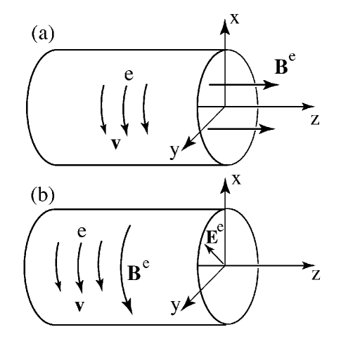
Figure 1: Geometry of relativistic E-layer in (a) for the case of a uniform external axial magnetic field, and in (b) for an external toroidal magnetic field with an external radial electric field.

The equations for the self-fields are

$$\frac{1}{r}\frac{d}{dr}\left(r{d\Phi^{s}\over dr}\right)=4\pi e\int d^{3}p~{}f^{0}(H,P_{\phi})~{},$$ (4)

$$\frac{d}{dr}\left(\frac{1}{r}\frac{d(rA_{\phi}^{s})}{dr}\right)=4\pi e\int d^{3}p~{}v_{\phi}~{}f^{0}(H,P_{\phi})~{},$$ (5)

where $v_{\phi}=(P_{\phi}/r+eA_{\phi})/H$.

Owing to the small radial thickness of the layer, we can expand radially near $r_{0}$

$$\left[{P_{\phi}\over r}+eA_{\phi}(r)\right]^{2}\!\!\!=\left[{P_{\phi}\over r_{0}}\!\!+eA_{\phi}(r_{0})\right]^{2}\!\!+\delta rD_{1}\!\!+\!{1\over 2}\delta r^{2}D_{2},$$ (6)

where $D_{1}$, $D_{2}$ are the derivatives evaluated at $r_{0}$, and $\delta r\equiv r-r_{0}$ with $(\delta r/r_{0})^{2}\ll 1$. We choose $r_{0}$ so as to eliminate the term linear in $\delta r$. Thus,

$$H=H_{0}-e\Phi^{s}(r_{0})+{1\over 2H_{0}}\big{(}p_{r}^{2}+p_{z}^{2}+H_{0}^{2}~{}\omega_{\beta r}^{2}~{}\delta r^{2}\big{)}~{},$$ (7)

where $\omega_{\beta r}$ is the radial betatron frequency, and

$$H_{0} \equiv m_{e}\left\{1+\left[{P_{\phi}\over r_{0}}+eA_{\phi}(r_{0})\right]^{2}\right\}^{1/2}~{},$$ (8)

$$\gamma_{0} \equiv {H_{0}\over m_{e}}~{},$$

$$v_{\phi 0} \equiv {1\over H_{0}}\left[{P_{\phi}\over r_{0}}+eA_{\phi}(r_{0})\right]~{}.$$

We assume $\gamma_{0}^{2}\gg 1$ and $v_{\phi 0}>0$ so that $v_{\phi 0}=1-1/(2\gamma_{0}^{2})$ to a good approximation. The “median radius” $r_{0}$ is determined by the condition

$${D_{1}\over 2H_{0}}-e~{}{d\Phi^{s}\over dr}\bigg{|}_{r_{0}}=0~{},$$

or

$${1\over H_{0}}\left({P_{\phi}\over r_{0}}+eA_{\phi}\right)\left(-{P_{\phi}\over r_{0}^{2}}+e~{}{dA_{\phi}\over dr}\right)\bigg{|}_{r_{0}}=e~{}{d\Phi^{s}\over dr}\bigg{|}_{r_{0}}.$$ (9)

To a good approximation,

$$r_{0}={m_{e}\gamma_{0}v_{\phi 0}\over(1-2\zeta)eB^{e}_{z}}\approx{m_{e}\gamma_{0}\over eB^{e}_{z}}(1+2\zeta)\quad{\rm or}$$

$$r_{0}^{2}={2P_{\phi}\over eB^{e}_{z}}[1+3\zeta+{\cal O}(\zeta^{2})]~{}.$$ (10)

Here,

$$\zeta\equiv-~{}{B_{z}^{s}(r_{0})\over B^{e}_{z}}~{},\quad\quad{\rm with}\quad\quad\zeta^{2}\ll 1~{},$$ (11)

is the field-reversal parameter of Christofilos. For a radially thin E-layer of axial length $L$ consisting of a total number of electrons $N$, the surface density of electrons is $\sigma=N/(2\pi r_{0}L)$ and the surface current density is $-ev_{\phi}\sigma$. Because $B_{z}^{s}(r_{0})$ is one-half the full change of the self-magnetic field across the layer, we have $\zeta=r_{e}N/(\gamma L)$, where $r_{e}=e^{2}/(mc^{2})$ is the classical electron radius. Notice that $N$, $\zeta$, and $\gamma L$ are invariants under a Lorentz transform in the $z-$direction.

The radial betatron frequency $\omega_{\beta r}$ is given by

$$H_{0}^{2}~{}\omega_{\beta r}^{2}={D_{2}\over 2}-{D_{1}^{2}\over 4H_{0}^{2}}-H_{0}e{d^{2}\Phi^{s}\over dr^{2}}~{}.$$ (12)

Using Eq. (9) gives

$$\omega_{\beta r}^{2}={1-4\zeta\over 1-2\zeta}~{}{v_{\phi 0}^{2}\over r_{0}^{2}}~{}+{ev_{\phi 0}\over\gamma_{0}m_{e}}~{}{d^{2}A_{\phi}\over dr^{2}}\bigg{|}_{r_{0}}\!-{e\over\gamma_{0}m_{e}}~{}{d^{2}\Phi^{s}\over dr^{2}}\bigg{|}_{r_{0}}$$

$$\approx{1-2\zeta\over r_{0}^{2}}-{\sqrt{2/\pi}~{}\zeta\over r_{0}\Delta r\gamma^{2}}~{}.$$ (13)

The term $\propto 1/\Delta r$ is the sum of the defocusing self-electric force and the smaller focusing self-magnetic force. For the layer to be radially confined we need to have $\zeta<\sqrt{\pi/2}~{}\gamma^{2}(\Delta r/r_{0})$. For $\zeta\ll\gamma^{2}(\Delta r/r_{0})$ and $\zeta^{2}\ll 1$, we have $\omega_{\beta r}=1/r_{0}$ to a good approximation.

The number density follows from Eq. (3),

$$n\approx n_{0}\exp\left(-{\delta r^{2}\over 2\Delta r^{2}}\right)~{}~{}{\rm where}~{}~{}\Delta r\equiv\left({T\over H_{0}\omega_{\beta r}^{2}}\right)^{1/2}$$

$${\rm or}~{}~{}{\Delta r^{2}\over r_{0}^{2}}\simeq{v_{th}^{2}\over 1-2\zeta-\sqrt{2/\pi}~{}\zeta(r_{0}/\Delta r)/\gamma^{2}}$$ (14)

where

$$v_{th}\equiv\left({T\over\gamma_{0}m_{e}}\right)^{1/2}$$ (15)

and

$$n_{0}=2\pi KH_{0}Tr_{0}^{-1}\exp\left(-\frac{H_{0}-e\Phi^{s}(r_{0})}{T}\right)~{}.$$ (16)

As mentioned we assume the layer to be radially thin with $(\Delta r/r_{0})^{2}\ll 1$. Consequently, equations (4) and (5) become

$${d^{2}\Phi^{s}\over dr^{2}} \approx 4\pi en_{0}~{}\exp\left(-{\delta r^{2}\over 2\Delta r^{2}}\right)~{},\quad\quad$$

$${d^{2}A_{\phi}^{s}\over dr^{2}} \approx 4\pi en_{0}~{}v_{\phi 0}~{}\exp\left(-{\delta r^{2}\over 2\Delta r^{2}}\right)~{}.$$ (17)

Thus we obtain

$$\zeta={-B^{s}_{z}(r_{0})\over B_{z}^{e}}={4\pi en_{0}v_{\phi 0}\Delta r\sqrt{\pi/2}\over B_{z}^{e}}$$ (18)

The equilibrium is thus seen to be determined by three parameters,

$$\zeta^{2}~{},\quad v_{th}^{2}~{},\quad{\rm and}\quad 1/\gamma_{0}^{2}~{},$$ (19)

which are all small compared with unity.

II.1.1 Equilibrium Orbits

From the Hamiltonian of Eq. (7) we have

$$\!{d^{2}\delta r\over dt^{2}}\!=-\omega_{\beta r}^{2}\delta r,~{}\rightarrow~{}\delta r(t^{\prime})\!=\delta r_{i}\sin[\omega_{\beta r}(t^{\prime}-t)+\varphi]~{},$$ (20)

where $r-r_{0}=\delta r_{i}\sin\varphi$. For future use we express the orbit so that ${\bf r}(t^{\prime}=t)={\bf r}$, where $({\bf r},t)$ is the point of observation. Also, we have

$${d\phi\over dt}={P_{\phi}+erA_{\phi}(r)\over m_{e}\gamma r^{2}}=\dot{\phi}(r_{0})+{d\dot{\phi}\over dr}\bigg{|}_{r_{0}}\delta r+..~{},$$ (21)

so that

$$\phi(t^{\prime})=\phi+(t^{\prime}-t)\dot{\phi}_{0}+{1\over\omega_{\beta r}}{\partial\dot{\phi}_{0}\over\partial r}\bigg{|}_{r_{0}}\times$$

$$\bigg{\{}-\delta r_{i}\cos[\omega_{\beta r}(t^{\prime}-t)+\varphi]+\delta r_{i}\cos(\varphi)\bigg{\}}~{},$$ (22)

where $\partial\dot{\phi}/\partial r|_{r_{0}}=-\dot{\phi}_{0}/r_{0}$. For $\zeta\ll\gamma^{2}(\Delta r/r_{0})$ and $\zeta^{2}\ll 1$, we have $\partial\dot{\phi}/\partial r|_{r_{0}}/\omega_{\beta r}=-1/r_{0}$ to a good approximation. Because the E-layer is uniform in the $z-$direction,

$$z(t^{\prime})=z+(t^{\prime}-t)v_{z}~{}.$$ (23)

The orbits are necessary for the stability analysis.

II.2 Configuration b

Here, we describe a Vlasov equilibrium for an axisymmetric, long, thin cylindrical layer of relativistic electrons where the electron motion is almost parallel to the magnetic field. The equilibrium distribution function $f^{0}$ is again taken to be given by Eq. (3) in terms of the Hamiltonian, $H$, and the canonical angular momentum, $P_{\phi}\equiv rp_{\phi}-erA_{\phi}(r),$ where $A_{\phi}=A_{\phi}^{s}$. We make the same assumptions as above, $\gamma^{2}\gg 1$, $T/(m_{e}\gamma)\ll 1$, and $\Delta r^{2}/r_{0}^{2}\ll 1$. In this case there is no external $B_{z}$ field. Instead, we include an external toroidal magnetic field $B_{\phi}^{e}$ with corresponding vector potential $A_{z}^{e}$ and an external electric field ${\bf E}^{e}$ with potential $\Phi^{e}$. The fields ${\bf B}^{e}$ and ${\bf E}^{e}$ correspond to the magnetic and electric fields of a distant, charged, current-carrying flow along the axis. Thus, $|{E}^{e}_{r}|<|{B}_{\phi}^{e}|$. The considered external field is of course just one of a variety of fields which give electron motion almost parallel with the magnetic field. Note also that the distribution function is restricted in the respect that it does not include a dependence on the canonical momentum in the $z-$direction $P_{z}=m_{e}\gamma v_{z}-eA_{z}$.

The distribution function (3) gives $J_{z}=0$ so that there is no toroidal self magnetic field. Thus the self-potentials in this case are also given by equations (4) and (5). Equations (6) - (9) are also applicable with the replacement of $\Phi^{s}$ by the total potential $\Phi$. In place of Eq. (10) we find

$$r_{0}={m_{e}\gamma v_{\phi}^{2}\over(1-2\zeta)eE_{r}^{e}(r_{0})}\approx{m_{e}\gamma\over eE_{r}^{e}(r_{0})}(1+2\zeta)~{},$$ (24)

where $\zeta\equiv{B_{z}^{s}(r_{0})/E_{r}^{s}(r_{0})}.$ We again have $\zeta=r_{e}N/(\gamma L)$, where $r_{e}=e^{2}/(mc^{2})$ is the classical electron radius and $L$ is the axial length of the layer. Because $d^{2}\Phi^{e}/dr^{2}=-(1/r)d\Phi^{e}/dr$, the radial betatron frequency is again given by Eq. (13) (with $\Phi$ now the total potential) so that the orbits given in §2.1.1 also apply in this case. The electron motion is almost parallel to the magnetic field in that $(B_{z}^{s}/B_{\phi}^{e})^{2}=\zeta^{2}(E_{r}^{e}/B_{\phi}^{e})^{2}<\zeta^{2}\ll 1$. Notice that Eq. (24) for $r_{0}$ is formal in the respect that $E_{r}^{e}\propto 1/r$. Therefore, $r_{0}$ is in fact arbitrary in this case. Because the wavelengths of the unstable modes are found to be small compared with $r_{0}$, it may be interpreted as local radius of curvature of the magnetic field.

III Linear Perturbation

We now consider a general perturbation of the Vlasov equation with $f({\bf r,p},t)=f^{0}({\bf r,p})+\delta f({\bf r,p},t)$. To first order in the perturbation amplitude $\delta f$ obeys

$$\left({\partial\over\partial t}+{\bf v\cdot}{\partial\over\partial{\bf r}}+{d{\bf p}\over dt}~{}{\bf\cdot}~{}{\partial\over\partial{\bf p}}\right)\delta f\equiv{D\delta f\over Dt}=\quad\quad\quad$$

$$e(\delta{\bf E}+{\bf v\times}\delta{\bf B})~{}{\bf\cdot}~{}{\partial f^{0}\over\partial{\bf p}}~{},$$ (25)

where $\delta{\bf E}$ and $\delta{\bf B}$ are the perturbations in the electric and magnetic fields. All scalar perturbation quantities are considered to have the dependencies

$$F(r)\exp(im\phi+ik_{z}z-i\omega t)~{},$$ (26)

where the angular frequency $\omega$ is taken to have at least a small positive imaginary part which corresponds to a growing perturbation. This allows for a correct initial value treatment of the problem (Landau, 1946). For a perturbation taken to vanish as $t\to-\infty$,

$$\delta f({\bf r,p},t)=$$

$$e\int_{-\infty}^{t}dt^{\prime}\bigg{\{}\delta{\bf E}[{\bf r}(t^{\prime}),t^{\prime}]+{\bf v}(t^{\prime}){\times}\delta{\bf B}[{\bf r}(t^{\prime}),t^{\prime}]\bigg{\}}~{}{\bf\cdot}~{}{\partial f^{0}\over\partial{\bf p}}~{},$$ (27)

where the integration follows the orbit $[{\bf r}(t^{\prime}),{\bf p}(t^{\prime})]$ which passes through the phase-space point $[{\bf r},{\bf p}]$ at time $t$. For the considered axisymmetric equilibria,

$${\partial f^{0}\over\partial{\bf p}}={{\bf p}\over H}\left.{\partial f^{0}\over\partial H}\right|_{P_{\phi}}+r\hat{{\hbox{\tenbg\char 30\relax}}~{}}\left.{\partial f^{0}\over\partial P_{\phi}}\right|_{H}~{},$$ (28)

where the partial derivatives are to be evaluated at constant $P_{\phi}$ and $H$, respectively. Thus, the right-hand side of Eq. (25) becomes

$$e\left(-{d\delta\Phi\over dt}+i\omega(\dot{\phi}~{}\delta\Psi-\delta\Phi)+i\omega{\bf v}_{\perp}\cdot\delta{\bf A}\right){\partial f^{0}\over\partial H}+$$

$$e\left(-{d\delta\Psi\over dt}+im(\dot{\phi}~{}\delta\Psi-\delta\Phi)+im{\bf v}_{\perp}\cdot\delta{\bf A}\right){\partial f^{0}\over\partial P_{\phi}}~{},$$ (29)

where $\delta{\bf E}=-{\bf\nabla}\delta\Phi-\partial{\bf\delta A}/\partial t$ and $\delta{\bf B}={\nabla\times}{\bf\delta A}$, $\delta\Psi\equiv r\delta A_{\phi}$ is the perturbation in the flux function, ${\bf v}_{\perp}=(v_{r},v_{z})$, and $d/dt=\partial/\partial t+{\bf v}\cdot{\bf\nabla}$. We assume the Lorentz gauge ${\bf\nabla\cdot}\delta{\bf A}+\partial\delta\Phi/\partial t=0$.

Evaluating Eq. (27) gives

$$\!\!\!\delta f=e{\partial f^{0}\over\partial H}\left[-\delta\Phi+i\omega\int_{-\infty}^{t}\!\!\!\!\!dt^{\prime}\left(\dot{\phi}^{\prime}\delta\Psi^{\prime}-\delta\Phi^{\prime}+{\bf v}^{\prime}_{\perp}\cdot\delta{\bf A}^{\prime}\right)\right]$$

$$+e{\partial f^{0}\over\partial P_{\phi}}\left[-\delta\Psi+im\int_{-\infty}^{t}\!\!\!\!dt^{\prime}~{}\left(\dot{\phi}^{\prime}\delta\Psi^{\prime}-\delta\Phi^{\prime}+{\bf v}^{\prime}_{\perp}\cdot\delta{\bf A}^{\prime}\right)\right]~{},$$ (30)

where the prime indicates evaluation at $[{\bf r}(t^{\prime}),t^{\prime}]$. The integration is along the unperturbed particle orbit so that $\partial f^{0}/\partial H$ and $\partial f^{0}/\partial P_{\phi}$ are constants and can be taken outside the integrals. Note also that $d/dt$ acting on a function of $({\bf r},t)$ is the same as $D/Dt$.

IV First Approximation

As a starting approximation we neglect (i) the radial oscillations in the orbits [$(\Delta r/r_{0})^{2}\ll 1$], (ii) the self-field corrections to orbits proportional to $\zeta$, (iii) the terms in $\delta f$ proportional to $v_{\perp}^{2}$ ($v_{th}^{2}\approx(\Delta r/r_{0})^{2}\ll 1$), (iv) we take $k_{z}=0$ and (v) we assume the layer is very thin. Owing to approximation (iii), we can neglect the terms $\propto{\bf v}_{\perp}\cdot\delta{\bf A}$ in Eq. (30) in the evaluation of $\delta\rho$ and $\delta J_{\phi}$. This is because these terms give contributions to $\delta f$ which are odd functions of $v_{r}$ and $v_{z}$. Therefore, their average contribution can be neglected.

Evaluation of Eq. (30) gives

$$\delta f=-e{\partial f^{0}\over\partial H}\bigg{|}_{P_{\phi}}\!\!\!{\dot{\phi}(\omega\delta\Psi-m\delta\Phi)\over\omega-m\dot{\phi}}-e{\partial f^{0}\over\partial P_{\phi}}\bigg{|}_{H}{\omega\delta\Psi-m\delta\Phi\over\omega-m\dot{\phi}}~{},$$ (31)

where $\dot{\phi}=\dot{\phi}(r_{0})$. The approximations lead to a closed system with potentials $(\delta\Phi,~{}\delta\Psi)$ and sources $(\delta\rho,~{}\delta J_{\phi})$.

We have

$$\delta\rho=-e\int d^{3}p~{}\delta f=-{e\over r_{0}}\int dp_{r}dp_{z}dP_{\phi}~{}\delta f~{},~{}~{}~{}$$

$$\delta J_{\phi}=-e\int d^{3}p~{}v_{\phi}\delta f=-{e\over r_{0}}\int dp_{r}dp_{z}dP_{\phi}~{}v_{\phi}\delta f~{}.$$ (32)

For the considered distribution function, Eq. (3), $\partial f^{0}/\partial H=-f^{0}/T$. The $\partial f^{0}/\partial P_{\phi}$ term in Eq. (31) can be integrated by parts. Furthermore, note that $\partial H/\partial P_{\phi}=\dot{\phi}$ and $\partial\dot{\phi}/\partial P_{\phi}=-(\dot{\phi})^{2}/H$, which corresponds to an effective “negative mass” for the particle’s azimuthal motion (Kolomenskii & Lebedev, 1959; Nielson et al., 1959; Lawson, 1988). From the partial integration the small term proportional to $\partial v_{\phi}/\partial P_{\phi}=v_{\phi}/(r_{0}H^{3})$ is neglected. Also note that $H$ is not a constant when performing the integration over momenta. Evaluating this term by an integration by parts with a general function $g(P_{\phi})$ in the integrand gives

$$\int dP_{\phi}\left.\frac{\partial f^{0}}{\partial P_{\phi}}\right|_{H}g(P_{\phi})=$$ (33)

$$- K\int dP_{\phi}\delta(P_{\phi}-P_{0})\frac{\partial}{\partial P_{\phi}}\left[g(P_{\phi})e^{-H/T}\right]=$$

$$- K\int dP_{\phi}\delta(P_{\phi}-P_{0})\frac{\partial}{\partial P_{\phi}}\left[g(P_{\phi})\right]e^{-H/T}$$

$$+ \frac{K}{T}\int dP_{\phi}\delta(P_{\phi}-P_{0})g(P_{\phi})e^{-H/T}\frac{\partial H}{\partial P_{\phi}}~{}.$$

That is, the integration produces an additional term which cancels the $1/T$-term. Thus,

$$\int dP_{\phi}\delta f=-e\int dP_{\phi}{f^{0}\over H}~{}{m\dot{\phi}^{2}(\omega\delta\Psi-m\delta\Phi)\over(\Delta\omega)^{2}}~{},$$ (34)

where $\Delta\omega\equiv\omega-m\dot{\phi}$. Integrating over the remaining momenta gives

$$(\delta\rho,~{}\delta J_{\phi})=(1,v_{\phi})~{}e^{2}~{}n(r){m\dot{\phi}^{2}\over H}\cdot{(\omega\delta\Psi-m\delta\Phi)\over(\Delta\omega)^{2}}~{}.$$ (35)

For a radially thin E-layer we may take $n(r)=n_{0}\exp(-\delta r^{2}/2\Delta r^{2})\rightarrow n_{0}\sqrt{2\pi}\Delta r~{}\delta(\delta r)$. We comment on this approximation below in more detail when we include the radial wavenumber $k_{r}$ of the perturbation. Then equations (100) and (101) can be written as

$$[\delta\Phi(r_{0}),~{}\delta\Psi(r_{0})]=\big{[}1,~{}r_{0}v_{\phi}(1+\Delta\tilde{\omega})\big{]}~{}2\pi^{2}r_{0}~{}Z\int dr~{}\delta\rho(r)~{},$$ (36)

where $Z\equiv iJ_{m}(\omega r_{0})H_{m}^{(1)}(\omega r_{0})$, $\tilde{\omega}\equiv\omega/(m\dot{\phi})$ and $\Delta\tilde{\omega}\equiv\Delta\omega/(m\dot{\phi})$. Integrating Eq. (35) over the radial extent of the E-layer and cancelling out the field amplitudes gives the dispersion relation

$$1=2\pi^{2}r_{0}~{}[n_{0}e^{2}\sqrt{2\pi}\Delta r]~{}Z{m\dot{\phi}^{2}\over H}\cdot{\omega r_{0}v_{\phi}(1+\Delta\tilde{\omega})-m\over(\Delta\omega)^{2}}~{}.$$ (37)

In terms of dimensionless variables this becomes

$$1=\pi~{}\zeta~{}Z~{}\left(2\Delta\tilde{\omega}-{1\over\gamma^{2}}\right){1\over(\Delta\tilde{\omega})^{2}}~{},$$ (38)

where $Z=iJ_{m}(m\tilde{\omega}v_{\phi})H_{m}^{(1)}(m\tilde{\omega}v_{\phi})$, $H^{(1)}_{m}=J_{m}+iY_{m}$, and the field-reversal parameter $\zeta=4\pi en_{0}v_{\phi}\Delta r\sqrt{\pi/2}/B^{e}_{z}$ as given by Eq. (11).

For $m\gg 1$, $J_{m}(m\tilde{\omega}v_{\phi})\approx(2/m)^{1/3}{\rm Ai}(w)$ and $Y_{m}(m\tilde{\omega}v_{\phi})\approx-(2/m)^{1/3}{\rm Bi}(w)$, where ${\rm Ai}$ and ${\rm Bi}$ are the Airy functions and $w=(m/2)^{2/3}(\gamma^{-2}-2\Delta\tilde{\omega})$ Abramowitz & Stegun (1965). Thus we have $Z=iJ_{m}H_{m}^{(1)}\approx(2/m)^{2/3}[{\rm Ai}(w){\rm Bi}(w)+i{\rm Ai}^{2}(w)]$. It is useful to denote $Z$ as $Z_{m}(w)$. For $|w|^{2}\gg 1$, ${\rm Ai}(w)\approx(2\sqrt{\pi})^{-1}w^{-1/4}\exp(-2w^{3/2}/3)$, ${\rm Bi}(w)\approx(\sqrt{\pi})^{-1}w^{-1/4}\exp(2w^{3/2}/3)$, $Z_{m}\approx(2/m)^{2/3}/(2\pi|w|^{1/2})$.

For $|w|^{2}\lesssim 0.5$, ${\rm Ai}(w)=c_{1}-c_{2}w+{\rm O}(w^{3})$ and ${\rm Bi}(w)=\sqrt{3}[c_{1}+c_{2}w+{\rm O}(w^{3})]$, where $c_{1}=1/[3^{2/3}\Gamma(2/3)]\approx 0.355$ and $c_{2}=1/[3^{1/3}\Gamma(1/3)]\approx 0.259$. In this limit we have $Z_{m}(w)\approx(2/m)^{2/3}[\sqrt{3}(c_{1}^{2}-c_{2}^{2}w^{2})+i(c_{1}-c_{2}w)^{2}]$. For $|w|^{2}\ll 1$, $Z_{m}\approx(0.347+0.200~{}i)/m^{2/3}$.

IV.1 Range of Validity

We are interested in the regime where the wavelength of the emitted radiation is comparable to the “bunch length”, i.e. $\omega\approx m$ or equivalently $\Delta\tilde{\omega}\ll 1$. However, Eq. 38 is only valid if $\Delta\tilde{\omega}\ll\gamma^{-2}$. Since we neglected $\delta J_{r}$ and $\delta J_{z}$ we obtain from the continuity equation $\delta J_{\phi}=\frac{\omega r_{0}}{m}\delta\rho$. Due to this approximation the factor on the right hand side can become bigger than the speed of light if $\Delta\tilde{\omega}>\gamma^{-2}$ which leads to unphysical results. In the latter case $\delta J_{\phi}=v_{\phi}\delta\rho$ is a better approximation. Fortunately, $\Delta\tilde{\omega}\ll\gamma^{-2}$ is the most interesting case and in the remainder of this paper we will always work in this limit. Furthermore, for the continuum approximation to be valid the mean particle distance has to be much smaller than the wavelength.

IV.2 Growth Rates

It will prove useful to define two characteristic values of $m$: $m_{1}\equiv\zeta^{3/2}\gamma^{3}$ and $m_{2}=2\gamma^{3}$, and therefore $m_{1}=\zeta^{3/2}m_{2}/2$. We can obtain approximate solutions to Eq. (38) in two different cases. There may be solutions with small values of $\gamma^{2}\Delta\tilde{\omega}$, so that $w\simeq(m/m_{2})^{2/3}$. In this case, Eq. (38) becomes a simple quadratic equation, which can be solved for $\Delta\tilde{\omega}$. We can simplify the solution somewhat by changing variables to $\sigma\equiv\gamma^{2}\Delta\tilde{\omega}$ in which case Eq. (38) can be written in the form

$$1={\pi\zeta Z_{m}\gamma^{2}\over\sigma^{2}}(\sigma-1)\approx-{\pi\zeta Z_{m}\gamma^{2}\over\sigma^{2}},$$

where we have neglected $\sigma$ compared to one in the approximate version of this equation. We find that

$$\sigma\simeq\sqrt{-\pi\zeta Z_{m}\gamma^{2}}~{}.$$ (39)

For case I let us assume that $m\ll m_{2}$, in which case Eq. (39) implies

$$\sigma\simeq\pm 1.121(m_{1}/m)^{1/3}~{}e^{i(7\pi/12)}$$

$$=1.121(m_{1}/m)^{1/3}(-0.2588+0.9659i)~{}.$$ (40)

so $|\sigma|\ll 1$ for $m\gg m_{1}$. The growth rate of the unstable mode is

$$\omega_{i}\simeq{1.083\zeta^{1/2}m^{2/3}\dot{\phi}\over\gamma}$$ (41)

in this regime. For case II we assume that $m\gg m_{2}$, in which case Eq. (39) implies

$$\sigma=\pm{i\zeta^{1/2}\gamma^{3/2}\over m^{1/2}}=\pm i\zeta^{1/2}(m_{2}/2m)^{1/2}$$

$$\omega_{i}\simeq{\zeta^{1/2}m^{1/2}\dot{\phi}\over\gamma^{1/2}}~{};$$ (42)

note that the growth rates in cases I and II match almost exactly at $m=m_{2}$, where $|\sigma|\approx\zeta^{1/2}$.

Note that $m_{2}\dot{\phi}$ is the approximate frequency of the peak of the single particle synchrotron radiation spectrum. For more accurate results we employ a numerical method for solving Eq. 38 outlined in Botten et al. (1983). This method also allows us to count the number of roots which are enclosed by a contour. So far we have no numerical evidence of the existence of more than one solution with a positive real part. The numerical results agree very well with our approximations even if $m<m_{1}$ and are shown in Fig. 2.

IV.3 Comparison with Goldreich and Keeley

Goldreich and Keeley Goldreich & Keeley (1971) find a radiation instability in a thin ring of relativistic, monoenergetic, zero temperature electrons constrained to move in a circle of fixed radius. Under the condition $1\ll m^{1/3}\ll\gamma$ their growth rate is $\omega_{i}\approx 1.16\dot{\phi}~{}m^{2/3}[r_{e}N/(\gamma^{3}r_{0})]^{1/2}$ which is close to our growth rate with $L$ replaced by $r_{0}$.

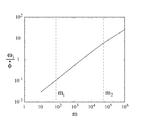
Figure 2: The graph shows the frequency dependence of the growth rate for a sample case where $\gamma=30$ and $\zeta=0.02$ obtained from our approximations for Eq. (38). For these parameters, $m_{1}\approx 10^{2}$ and $m_{2}\approx 2.7\times 10^{4}$.

V Nonlinear Saturation

Clearly the rapid exponential growth of the linear perturbation can continue only for a finite time. We analyze this by studying the trapping of electrons in the moving potential wells of the perturbation. For $(\Delta r/r_{0})^{2}\ll 1$, the electron orbits can be treated as circular. The equation of motion is

$${dP_{\phi}\over dt}=r\delta F_{\phi}~{},\quad\delta F_{\phi}=-e[\delta E_{\phi}+({\bf v\times}\delta{\bf B})_{\phi}]~{},$$ (43)

where $P_{\phi}$ is the canonical angular momentum, where

$$\delta F_{\phi}=-e\delta E_{\phi 0}\exp(\omega_{i}t)\cos(m\phi-\omega_{r}t)~{},\!\!$$ (44)

where $\delta E_{\phi 0}$ is the initial value of the potential, $\omega_{r}\equiv{\rm Re}(\omega)$, and $\omega_{i}\equiv{\rm Im}(\omega)$.

For a relativistic particle in a circular orbit,

$$\delta P_{\phi}=m_{e*}r_{0}^{2}\delta\dot{\phi},~{}~{}{\rm where}~{}m_{e*}={-m_{e}\gamma^{3}\over\gamma^{2}-1}\approx-m_{e}\gamma,$$ (45)

where $m_{e*}$ is the “effective mass,” which is negative, for the azimuthal motion of the electron (Kolomenskii & Lebedev (1959); Nielson et al. (1959) or Lawson (1988), p.68). Combining equations (43) and (45) gives

$${d^{2}\varphi\over dt^{2}}=-\omega_{T}^{2}(t)\sin\varphi~{},$$ (46)

where $\varphi\equiv m\phi-\omega_{t}t+\frac{3}{2}\pi$, $\omega_{T}\equiv\omega_{T0}\exp(\omega_{i}t/2),$ and $\omega_{T0}\equiv[em\delta E_{\phi 0}/(m_{e}\gamma r_{0})]^{1/2}$, where $\omega_{T}$ is termed the “trapping frequency.” At the “bottom” of the potential well of the wave, $\sin\varphi\approx\varphi$. An electron oscillates about the bottom of the well with an angular frequency $\sim\omega_{T}$. This is of course a nonlinear effect of the finite wave amplitude. A WKBJ solution of Eq. (45) gives

$$\varphi\propto\omega_{T0}^{-1/2}\exp(-\omega_{i}t/4)\sin\big{\{}(2\omega_{T0}/\omega_{i})[\exp(\omega_{i}t/2)-1]\big{\}}~{}.$$ (47)

The exponential growth of the linear perturbation will cease at the time $t_{sat}$ when the particle is turned around in the potential well. This condition corresponds to $\omega_{T}(t_{sat})\approx\omega_{i}$. Thus, the saturation amplitude is

$$\big{|}\delta E_{sat}\big{|}^{2}=\left(\frac{m_{e}\gamma}{er_{0}m}\right)^{2}\left({\omega_{i}(m)\over\dot{\phi}}\right)^{4}~{},$$ (48)

where $|\delta E_{sat}|\equiv|\delta E(t_{sat})|=|\delta E_{0}|\exp(\omega_{i}t_{sat})$.

VI First Approximation with $k_{z}\neq 0$

Here, we consider $k_{z}\neq 0$ but keep the other approximations. Our ansatz for $\delta f$ is general enough to handle this case since it retains the biggest contribution to the Lorentz force in the $z$-direction which is of the order $v_{\phi}B_{r}$. In place of Eq. (34) we obtain

$$\int dP_{\phi}\delta f=-e\int dP_{\phi}{f^{0}\over H}~{}{m\dot{\phi}^{2}(\omega\delta\Psi-m\delta\Phi)\over(\omega-m\dot{\phi}-k_{z}v_{z})^{2}}~{},$$ (49)

where we assume without loss of generality $k_{z}>0$ and $k_{z}\ll m/r_{0},\omega$. In place of Eq. (38) we find

$$\varepsilon(\omega,k_{z})=1\!+k_{z}A(\omega,k_{z})\int_{-\infty}^{\infty}\!\!dv_{z}~{}{\exp(-v_{z}^{2}/2v_{th}^{2})\over\sqrt{2\pi}~{}v_{th}}\big{[}...\big{]}=0,$$ (50)

where

$$\big{[}...\big{]}\equiv-{m\dot{\phi}\over(\omega-m\dot{\phi}-k_{z}v_{z})^{2}}~{}.$$

Here, $\varepsilon$ acts as an effective dielectric constant for the E-layer, and

$$A(\omega,k_{z})\equiv\pi~{}\zeta~{}Z(\omega,k_{z})~{}\left(u-{k_{\phi}\over k_{z}\gamma^{2}}\right),~{}~{}u\equiv{\omega-m\dot{\phi}\over k_{z}}~{},$$

$$Z\equiv iJ_{m}[r_{0}(\omega^{2}-k_{z}^{2})^{1/2}]~{}H_{m}^{(1)}[r_{0}(\omega^{2}-k_{z}^{2})^{1/2}]~{},$$ (51)

and $k_{\phi}=m/r_{0}$ is the azimuthal wavenumber. The expression for $Z$ is from §4. An integration by parts gives

$$\varepsilon(u)=1+A(\omega)\int dv_{z}~{}{\exp(-v_{z}^{2}/2v_{th}^{2})\over\sqrt{2\pi}~{}v_{th}^{3}}{m\dot{\phi}v_{z}/k_{z}\over v_{z}-u}~{},$$ (52)

where the $k_{z}$ dependence of $\varepsilon$ and $A$ is henceforth implicit. We can also write this equation as

$$\varepsilon(u)=1+B(u)\left[1+\frac{u}{v_{th}}F\left({u\over v_{th}}\right)\right]~{},$$ (53)

where

$$B(u) \equiv {\pi\over v_{th}^{2}}~{}\zeta~{}Z~{}{k_{\phi}\over k_{z}}\left(u-{k_{\phi}\over k_{z}\gamma^{2}}\right)~{},$$ (54)

and

$$F(z)\equiv{1\over\sqrt{2\pi}}\int_{-\infty}^{\infty}dx~{}{\exp(-{x^{2}/2})\over x-z}~{},$$

for ${\rm Im}(z)>0$, and

$$F(z)\equiv{1\over\sqrt{2\pi}}\int_{-\infty}^{\infty}dx~{}{\exp(-{x^{2}/2})\over x-z}+i\sqrt{2\pi}\exp\left(-{z^{2}\over 2}\right)~{},$$

${\rm for~{}Im}(z)<0$. The second expression for $F(z)$ is the analytic continuation of the first expression to ${\rm Im}(z)<0$ which corresponds to wave damping (see, e.g., Montgomery & Tidman (1964), ch. 5). Note that terms of order $\Delta\tilde{\omega}$ have been omitted.

For $m\gg 1$, the factor $Z=iJ_{m}(J_{m}+iY_{m})$ can be expressed in terms of Airy functions in a way similar to that done in §5. One finds $J_{m}[r_{0}(\omega^{2}-k_{z}^{2})^{1/2}]\approx(2/m)^{1/3}{\rm Ai}(w)$, $Y_{m}[r_{0}(\omega^{2}-k_{z}^{2})^{1/2}]\approx-(2/m)^{1/3}{\rm Bi}(w)$,

$$Z_{r}\approx\left({2\over m}\right)^{2/3}{\rm Ai}(w){\rm Bi}(w)~{},~{}Z_{i}\approx\left({2\over m}\right)^{2/3}{\rm Ai}^{2}(w)~{},$$ (55)

where

$$\tan\psi\equiv{k_{z}\over k_{\phi}}~{},~{}w\equiv\left({m\over 2}\right)^{2/3}\left({1\over\gamma^{2}}+\tan^{2}\psi-2u\tan\psi\right)~{}.$$

It is clear that $\varepsilon$ has in general a rather complicated dependence on $u=u_{r}+iu_{i}$ and $\tan\psi$. Note that the expression for $w$ goes over to our earlier $w$ for $\psi=0$ noting that $u\tan\psi\rightarrow\Delta\tilde{\omega}$.

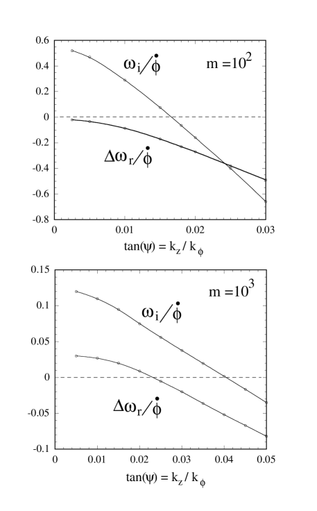
Figure 3: The figure shows the growth/damping rate $\omega_{i}$ and real part of the frequency $\Delta\omega_{r}=\omega-m\dot{\phi}$ in units of $\dot{\phi}$ as a function of $\tan\psi=k_{z}/k_{\phi}$ for $m=100$ and $m=1000$ for an E-layers with $\gamma=30$, $\zeta=0.02$ and $v_{th}=30/\gamma^{2}$. In the region of damping $\omega_{i}<0$, the second expression for $F(z)$ in Eq. (53) is used.

A limit where Eq. (53) can be solved analytically is for $|u|^{2}=|\Delta\tilde{\omega}|^{2}/\tan^{2}\psi\gg v_{th}^{2}$, that is, for sufficiently small $\tan\psi$. In this limit Eq. (53) can be expanded as an asymptotic series $F(z)=-1/z-1/z^{3}-3/z^{5}-..$. Keeping just the first three terms of the expansion gives

$$\varepsilon=1+\pi\zeta Z\left(1+{3v_{th}^{2}\tan^{2}\psi\over(\Delta\tilde{\omega})^{2}}\right){{\gamma^{-2}}\over(\Delta\tilde{\omega})^{2}}=0.$$ (56)

For $\tan\psi\rightarrow 0$ and $\Delta\tilde{\omega}\ll\gamma^{-2}$, this is the same as Eq. (38) as it should be. In general Eq. 56 will have more than one unstable mode. In the remainder of this paragraph we will only study the largest unstable solution for which we recover the growth rates found in §4 in the limit $\tan\psi\rightarrow 0$. Fig. 3 shows some sample solutions. For the case shown the $u$ dependence of $Z$ is negligible.

General solutions of Eq. (53) can be obtained using the Newton-Raphson method (Teukolsky et al. (1989), ch. 9) where an initial guess of $(u_{r},u_{i})$ gives $(\epsilon_{r},\epsilon_{i})$. This guess is incremented by an amount

$$\left[\begin{array}[]{c}{\delta u_{r}}\\ \vskip 6.0pt plus 2.0pt minus 2.0pt\cr{\delta u_{i}}\end{array}\right]~{}=~{}\left[\begin{array}[]{cc}{\partial\epsilon_{r}/\partial u_{r}}&{\partial\epsilon_{r}/\partial u_{i}}\\ \vskip 6.0pt plus 2.0pt minus 2.0pt\cr{\partial\epsilon_{i}/\partial u_{r}}&{\partial\epsilon_{i}/\partial u_{i}}\end{array}\right]^{-1}\left[\begin{array}[]{c}{-\epsilon_{r}}\\ \vskip 6.0pt plus 2.0pt minus 2.0pt\cr{-\epsilon_{i}}\end{array}\right]~{},$$ (63)

and the process is repeated until $\varepsilon_{r}=0$ and $\varepsilon_{i}=0$. Fortunately, the convergence is very rapid and gives $|\varepsilon|<10^{-10}$ after a few iterations.

Fig. 3 shows the dependence of the complex wave frequency on the tangent of the propagation angle, $\tan\psi=k_{z}/k_{\phi}$, for a sample cases. The maximum growth rate is for $\psi=0$ or $k_{z}=0$. With increasing $\psi$ the growth rate decreases, and for $\psi$ larger than a critical angle $\psi_{cr}$ there is damping. For the damping the second expression for $F$ in Eq. (53) must be used. Roughly, we find that the critical angle corresponds to having the wave phase velocity in the $z-$direction of the order of the thermal spread in this direction, that is, $u_{r}=\Delta\omega_{r}/k_{z}\sim v_{th}$. This gives

$$\tan\psi_{cr}\sim{\sqrt{\zeta}\over v_{th}\!~{}\!\gamma~{}m^{1/3}}=\left({r_{e}N\over v_{th}^{2}\gamma^{3}L}\right)^{1/2}\!{1\over m^{1/3}}\leq\frac{1}{\gamma^{2}v_{th}}~{},$$ (64)

for $m_{1}<m<m_{2}$. Note that the dimensionless parameter which determines the cut-off at $\tan\psi_{cr}$ is $\gamma^{2}v_{th}$. Our numerical calculations of $\psi_{cr}$ give a slightly faster dependence, $\tan\psi_{cr}\propto 1/m^{0.40}$ for this range of $m$. Fig. 4 shows the $m$-dependence of the critical angle. It is reasonable to assume that in a particle accelerator the weak focusing in the z-direction sets a low limit on $k_{z}$.

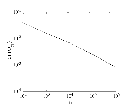
Figure 4: Critical angle for $\gamma=30$, $\zeta=0.02$ and $v_{th}=30/\gamma^{2}$.

VI.1 Nonlinear Saturation for $k_{z}\neq 0$

We generalize the results of §6 by including the axial as well as the azimuthal motion of the electrons in the wave. The axial equation of motion is

$$m_{e}\gamma{d^{2}z\over dt^{2}} = -e\left[\delta E_{z}+({\bf v}\times\delta{\bf B})_{z}\right]$$ (65)

$$\approx -e\delta E_{z0}\exp(\omega_{i}t)\cos(m\phi+k_{z}z-\omega t)~{}.$$

The approximation involves neglecting the force $\propto v_{r}\delta B_{\phi}$ which is valid for a radially thin layer ($\Delta r^{2}/r_{0}^{2}\ll 1$). Following the development of §6, the azimuthal equation of motion is

$$m_{e}\gamma r_{0}{d^{2}\phi\over dt^{2}}=-e\delta E_{z0}\cos(m\phi+k_{z}z-\omega t)~{}.$$ (66)

Combining equations (65) and (66) gives

$${d^{2}\varphi\over dt^{2}}=-~{}{e~{}m\delta E_{\phi 0}\over m_{e}\gamma r_{0}}\left(1+\tan^{2}\psi\right)\sin\varphi~{},$$ (67)

where $\varphi\equiv m\phi+k_{z}z-\omega t+\frac{3}{2}\pi$ and $\tan\psi=k_{z}/k_{\phi}$. Because $\psi^{2}\ll 1$ for wave growth (Eq. (64)), the saturation wave amplitude $\delta E_{sat}$ is again given by Eq. (48).

VII Thick Layers Including Radial Betatron Oscillations

VII.1 The Limit $k_{r}\Delta r\gg 1$

In this section we include the small but finite radial thickness of the E-layer. We keep the other approximations mentioned at the beginning of §5. In particular we consider $k_{z}=0$. In order to include the layer’s radial thickness, we consider the wave equations within the E-layer,

$$(\nabla^{2}+\omega^{2})\delta\Phi = -4\pi\delta\rho~{},$$

$$(\tilde{\nabla}^{2}+\omega^{2})\delta\Psi = -4\pi r\delta J_{\phi}~{},$$ (68)

where

$$\tilde{\nabla}^{2}\equiv{\partial^{2}\over\partial r^{2}}-{1\over r}{\partial\over\partial r}-\frac{m^{2}}{r^{2}}+{\partial^{2}\over\partial z^{2}}~{},$$ (69)

is the adjoint Laplacian operator.

Within the E-layer, we assume that the potentials can be written in a WKBJ expansion as

$$(\delta\Phi,~{}\delta\Psi)=(K_{\Phi},~{}K_{\Psi})\exp\big{[}im\phi+ik_{r}(r-r_{0})-i\omega t\big{]}~{},$$ (70)

where $k_{r}$ is the radial wavenumber with $(k_{r}\Delta r)^{2}\gg 1$ $(K_{\Phi},K_{\Psi})$ are constants. This is equivalent to assuming that the charge density is constant between $r_{0}-\Delta r$ and $r_{0}+\Delta r$ and zero elsewhere. Evaluation of the time integrals in Eq. (30) for $r=r_{0}$ gives

$$\int_{-\infty}^{t}dt^{\prime}\delta\Phi^{\prime}=\delta\Phi(r_{0},t)\times\quad\quad\quad$$

$$\sum_{n=-\infty}^{\infty}{J_{n}(k\delta r_{i})i^{n}\exp(-ik_{\phi}\delta r_{i}-in\psi)\over i(m\dot{\phi}+n\omega_{\beta r}-\omega)}~{},$$ (71)

where $n$ is an integer, $k\equiv(k_{r}^{2}+k_{\phi}^{2})^{1/2}$, with $k_{\phi}=m/r_{0}$, and $\tan\psi\equiv k_{r}/k_{\phi}$. There is an analogous expression for the integral of $\delta\Psi$. We have used Eq. (20) for the radial motion with $\varphi=0$ assuming $\zeta^{2}\ll 1$ and $\zeta\ll\gamma^{2}(\Delta r/r_{0})$ so that $\omega_{\beta r}=1/r_{0}$, and Eq. (22) for the $\phi$-motion with $\partial\dot{\phi}_{0}/\partial r|_{r_{0}}/\omega_{\beta r}=-1/r_{0}$. Using equations (30) and (71), the momentum space integrals (32) can be done to give

$$\left(eKe^{-H/T}\right)^{-1}\int dP_{\phi}\delta f=\frac{1}{T}(K_{\Psi}\dot{\phi}-K_{\Phi})\left\{J_{0}(k\delta r_{i})-1+(m\dot{\phi}-\omega)\sum_{n=-\infty}^{~{}~{}\infty~{}~{}\prime}\frac{i^{n}e^{-in\psi-ik_{\phi}\delta r_{i}}J_{n}(k\delta r_{i})}{m\dot{\phi}+n\omega_{\beta r}-\omega}\right\}-$$

$$\frac{m\dot{\phi}^{2}}{H}\frac{\omega K_{\Psi}-mK_{\Phi}}{(m\dot{\phi}-\omega)^{2}}-\frac{m\dot{\phi}^{2}}{H}m(K_{\Psi}\dot{\phi}-K_{\Phi})\left\{\frac{J_{0}(k\delta r_{i})-1}{(m\dot{\phi}-\omega)^{2}}+\sum_{n=-\infty}^{~{}~{}\infty~{}~{}\prime}\frac{i^{n}e^{-in\psi-ik_{\phi}\delta r_{i}}J_{n}(k\delta r_{i})}{(m\dot{\phi}+n\omega_{\beta r}-\omega)^{2}}\right\}~{},$$ (72)

and finally if $\Delta\tilde{\omega}\ll\gamma^{-2}$

$$\delta\rho\approx{e^{2}n_{0}m\dot{\phi}^{2}K_{\Phi}\over H}\bigg{(}{r_{0}^{2}\dot{\phi}\omega-m[1-(1-F_{0})/\gamma^{2}]\over(\omega-m\dot{\phi})^{2}}-{m\over\gamma^{2}}\sum_{n=-\infty}^{~{}~{}\infty~{}~{}\prime}{F_{n}\over(m\dot{\phi}+n\omega_{\beta r}-\omega)^{2}}\bigg{)}~{}.$$ (73)

The prime on the sums indicate that the $n=0$ term is omitted. Here,

$$F_{n}\equiv{i^{n}\exp(-in\psi)\over\sqrt{2\pi}\chi}\int_{-\infty}^{\infty}d\xi~{}J_{n}(\xi)\exp\left(-{\xi^{2}\over 2\chi^{2}}-i{k_{\phi}\xi\over k}\right)~{},$$ (74)

with

$$\chi\equiv k\Delta r~{}.$$ (75)

The $1/T$ terms in Eq. 73 do not cancel exactly. They may be neglected if

$$|\Delta\tilde{\omega}|^{2}\ll{F_{0}}v_{th}^{2}$$ (76)

for the $n=0$ term or if

$${|\Delta\tilde{\omega}|}|n/m-\Delta\tilde{\omega}|\ll{v_{th}^{2}}$$ (77)

for the $n\neq 0$ terms.

For weak E-layers we have for $\chi\rightarrow 0$, $F_{0}\rightarrow 1$ and $F_{n\neq 0}\rightarrow 0$. In this limit we recover the results of §4. For $\chi\gg 1$ and $1\ll k_{r}r_{0}\ll k_{\phi}r_{0}$, the Gaussian factor in the integrand of $F_{n}$ can be neglected so that one obtains

$$F_{n}\approx i^{n}e^{-in\psi}\frac{1}{\sqrt{2\pi}\chi}\frac{2k}{|k_{r}|}\cos\left(\frac{n\pi}{2}\right)~{},~{}~{}{\rm even}~{}n~{},$$

$$F_{n}\approx-i^{n}e^{-in\psi}\frac{1}{\sqrt{2\pi}\chi}\frac{2ik}{|k_{r}|}\sin\left(\frac{n\pi}{2}\right)~{},~{}~{}{\rm odd}\ n~{}.$$ (78)

An alternative approximation for $F_{n}$ can be obtained by using the integral representation of the Bessel function. The remaining integral can then be computed numerically more easily. In this way we find

$$F_{n}=\frac{i^{n}e^{-in\psi}}{2\pi}\int_{-\pi}^{\pi}d\theta\exp\left[-in\theta-(\chi^{2}/2)(k_{\phi}/k-\sin\theta)^{2}\right]~{}.$$ (79)

For $\chi\gg 1$, $1\ll(k_{\phi}/k_{r})^{2}$ and $|n|<\sqrt{\chi}$ we can approximate $\sin\theta$ in the exponent by a parabola at its maximum. We obtain

$$F_{n}\approx\frac{i^{n}e^{-in\psi}}{2^{3/4}\Gamma\left(\frac{3}{4}\right)\sqrt{\chi}}~{}.$$ (80)

In general $F_{n}/(i^{n}e^{-in\psi})$ decreases as $\chi$ and $n$ increase. This acts to prevent the unlimited increase of the growth rate as $m\longrightarrow\infty$, and it ensures that the sums over $n$ converge. Fig. 5 shows a plot of $F_{0}$ obtained by numerical evaluation of Eq. 79.

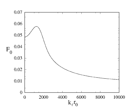
Figure 5: $F_{0}$ for $v_{th}=0.01$ and $k_{\phi}r_{0}=10^{4}$

Within the E-layer, Eq. (68) gives

$$k_{r}^{2}=\omega^{2}-{m^{2}\over r_{0}^{2}}\quad\quad\quad\quad\quad\quad\quad\quad\quad\quad\quad\quad\quad$$

$$+{4\pi e^{2}n_{0}m\dot{\phi}^{2}\over H}\bigg{(}{r_{0}^{2}\dot{\phi}\omega-m[1-(1-F_{0})/\gamma^{2}]\over(\omega-m\dot{\phi})^{2}}$$

$$-~{}{m\over\gamma^{2}}{\sum_{n}}^{\prime}{F_{n}\over(m\dot{\phi}+n\omega_{\beta r}-\omega)^{2}}\bigg{)}~{}.$$ (81)

In terms of dimensionless variables this equation becomes

$${\bar{k}_{r}}^{2}=2m^{2}\Delta\tilde{\omega}-\frac{m^{2}}{\gamma^{2}}+\quad\quad\quad\quad\quad\quad\quad\quad\quad\quad\quad$$

$$\frac{\zeta\sqrt{2}}{v_{\phi}v_{th}\sqrt{\pi}}\left(\frac{(1+\Delta\tilde{\omega})(1-\gamma^{-2})-[1+(F_{0}-1)/\gamma^{2}]}{(\Delta\tilde{\omega})^{2}}\right.$$

$$\left.-\frac{1}{\gamma^{2}}{\sum_{n}}^{\prime}\frac{F_{n}}{(v_{\phi}^{-1}n/m-\Delta\tilde{\omega})^{2}}\right)~{},\quad~{}~{}$$ (82)

where $\bar{k}_{r}\equiv r_{0}k_{r}$, $\bar{k}_{\phi}\equiv r_{0}k_{\phi}$, $\bar{k}\equiv r_{0}k$, and $\chi=\bar{k}v_{th}$.

Notice that Eq. 70 can also be written as

$$\delta\Phi=C_{2}\sin\big{[}k_{r}(r-r_{0})\big{]}+C_{3}\cos\big{[}k_{r}(r-r_{0})\big{]}~{},$$ (83)

for $r_{0}-\Delta r\leq r\leq r_{0}+\Delta r$. For $r\leq r_{0}-\Delta r$, we have

$$\delta\Phi=C_{1}J_{m}(\omega r)~{},$$ (84)

since the potential must be well behaved as $r\rightarrow 0$. For $r\geq r_{0}+\Delta r$, we must have

$$\delta\Phi=C_{4}\big{[}J_{m}(\omega r)+iY_{m}(\omega r)\big{]}~{}.$$ (85)

This combination of Bessel functions gives $\delta\Phi(r\rightarrow\infty)\rightarrow 0$ for the assumed conditions where ${\rm Im}(\omega)>0$. Note that these potentials are just the solutions of Eq. (68) in our approximation for $\delta\rho$. The eigenvalue problem can now be solved by matching the boundary conditions. However, we have not solved the full eigenvalue problem. Instead we consider unstable solutions with the restriction that $k_{r}\Delta r\gg 1$. Under this condition we can interpret Eq. 82 as a local dispersion relation. Unstable modes found from Eq. 82 will need a slight correction in order to satisfy the boundary conditions.

We expect that Eq. 82 has solutions near each betatron resonance at $\Delta\tilde{\omega}={\pm n}/{m}$. This is a familiar concept in the treatment of resonances in storage rings (cf. chao or schmekel ). We extract each solution by summing over a single value of $n$ and $-n$ only and obtain from Eq. 82 for the case $n\neq 0$ and $\Delta\tilde{\omega}\ll\gamma^{-2}$

$$\Xi\equiv-\frac{\gamma^{2}v_{th}\sqrt{\pi}\left(\bar{k}_{r}^{2}+m^{2}\gamma^{-2}\right)}{\zeta\sqrt{2}}=$$

$$\frac{F_{-n}}{\left(\frac{n}{m}+\Delta\tilde{\omega}\right)^{2}}+\frac{F_{n}}{\left(\frac{n}{m}-\Delta\tilde{\omega}\right)^{2}}~{}.$$ (86)

Thus,

$$\Delta\tilde{\omega}\approx\frac{F_{-n}-F_{n}}{\Xi}\pm\frac{n}{m}$$ (87)

for sufficiently big $\Xi$, i.e. we expect the imaginary part of $\Delta\tilde{\omega}$ to be negligible for the $n\neq 0$ modes. Despite a lot of effort we were not able to prove this statement under more relaxed conditions.

We can easily find an analytic solution of Eq. 82 for the case where the $n=0$ term is dominant. If $|\Delta\tilde{\omega}|\ll 1/\gamma^{2}$ and $|\Delta\tilde{\omega}|\ll F_{0}/\gamma^{2}$, we obtain

$$\Delta\tilde{\omega}=\pm\frac{2^{1/4}\sqrt{-\zeta F_{0}}}{\pi^{1/4}\sqrt{v_{th}(m^{2}+\gamma^{2}\bar{k}_{r}^{2})}}$$ (88)

The dependence of the growth rate on $k_{r}$ becomes significant when $\gamma^{2}\bar{k}_{r}^{2}/m^{2}$ is comparable to unity. For $m\sim m_{2}\sim\gamma^{3}$, we see that this happens when $(k_{r}\Delta r)^{2}/\gamma^{4}v_{th}^{2}\sim 1$, which involves the combination $\gamma^{2}v_{th}$ again.

The growth rate of Eq. 88 is proportional to $\sqrt{\zeta}$. This implies from §5 that the emitted power scales as the square of the number of particles in the E-layer which corresponds to coherent radiation. Sample results are shown in Fig. 6. We conclude that the main effect of the betatron oscillations is an indirect one. The radial motion itself is unimportant for the interaction. However, the influence of the radial motion on the time dependence of the azimuthal angle $\phi$ of a particle is important since a shift in $\phi$ can take the particle out of coherence with the wave. This effect is accounted for by $F_{0}$.

VII.2 Qualitative Analysis of the Effect of the Betatron Motion

Let us suppose that $v_{th}\gg 1/\gamma^{2}$, and that $|\Delta\tilde{\omega}|$ is not necessarily small compared with $v_{th}$ (We can still assume $|\Delta\tilde{\omega}|\ll 1$ without requiring the more restrictive condition $\gamma^{2}|\Delta\tilde{\omega}|\ll 1$.). The key effect of the betatron oscillations is to “wash out” the phase coherence of the response within the layer; for a cold layer, all orbiting particles move in “lock step”, which is particularly favorable for a bunching instability. Let us suppose that $|\Delta\tilde{\omega}|$ has a real part that is substantially larger than $1/\gamma^{2}$. The response in the layer scales as an Airy function with argument $w(1+\xi)$ where $|\xi|<v_{th}$. The phase accumulated across the layer thickness $\sim v_{th}r_{0}$ is $\eta\sim mv_{th}^{3/2}$ if $\Delta\tilde{\omega}_{r}\ll v_{th}$ and $\eta\sim mv_{th}^{3/2}(\Delta\tilde{\omega}_{r}/v_{th})^{1/2}$ if $\Delta\tilde{\omega}_{r}\gg v_{th}$. Large $\eta$ ought to imply substantial decoherence of the response in the layer. We see that this is likely irrespective of the value of $\Delta\tilde{\omega}_{r}/v_{th}$ provided that $m\gg v_{th}^{-3/2}$, i.e. for $m/\gamma^{3}\gg(\gamma^{2}v_{th})^{-3/2}$. At large values of $\gamma^{2}v_{th}$, phase smearing should suffice to suppress - if not eliminate - the bunching instability at frequencies near the synchrotron peak. Moreover, if $\gamma^{2}v_{th}\gtrsim\zeta^{-1}$, the instability should be suppressed over the entire range $m\gtrsim\zeta^{3/2}\gamma^{3}$ for which we found unstable modes in §4. Large $\Delta\tilde{\omega}_{r}/v_{th}$ would merely accentuate the smearing. At a given value of $m$, we see that $\Delta\tilde{\omega}_{r}\gtrsim(m^{2}v_{th}^{2})^{-1}$, i.e. $\gamma^{2}\Delta\tilde{\omega}_{r}\gtrsim(m/\gamma^{3})^{-1}(\gamma^{2}v_{th})^{-2}$ suffices for large phase decoherence in the layer.

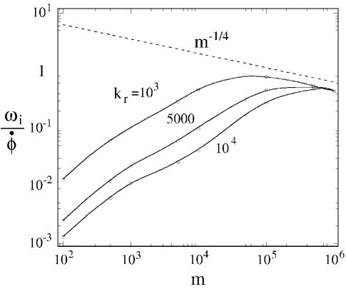
Figure 6: Growth rates in the limit $\bar{k}_{r}v_{th}\gg 1$ for our reference case $\gamma=30$, $\zeta=0.02$ and $v_{th}=1/\gamma^{2}$ and various values of $\bar{k}_{r}$. The line proportional to $m^{-1/4}$ is shown for comparison.

VII.3 The Limit $k_{r}\Delta r\ll 1$

In order to determine the lowest allowed value for $k_{r}$ and the highest possible growth rate the full eigenvalue problem has to be solved. We estimate the result by evaluating Eq. 100 in the thin approximation again. Looking at Eq. 100 and replacing the Bessel functions by their Airy function approximations for the case $m\gg m_{1}$ and $m\ll m_{2}$ we see that the thin approximation is justified if $\bar{k}_{r}v_{th}\ll 1$ and $m^{2/3}v_{th}\ll 1$. It starts to fail completely if $m^{2/3}v_{th}\gtrsim 1$, i.e. once we start integrating over the oscillating and/or the exponentially damped/increasing part of the Airy function, which implies we would like to have $m^{2/3}|\Delta\tilde{\omega}|\ll\sqrt{F_{0}}$ with $|\Delta\tilde{\omega}|^{2}\ll F_{0}v_{th}^{2}$ from the previous paragraph. However, for real values of $k_{r}$ we expect that the thin approximation will still give us an upper bound of the growth rate because it is easier to maintain coherence if all the radiation is emitted from the same orbit. With Eq. 73 we obtain in the limit $\Delta\tilde{\omega}\ll\gamma^{-2}$

$$1=-\pi~{}\zeta~{}Z~{}\frac{F_{0}\gamma^{-2}}{(\Delta\tilde{\omega})^{2}}~{},$$ (89)

The growth rates can be found as before. For $m\gg m_{1}$ we obtain

$$\omega_{i}\simeq{1.083\zeta^{1/2}m^{2/3}\dot{\phi}\over\gamma}\sqrt{F_{0}}$$ (90)

and

$$\omega_{i}\simeq{\zeta^{1/2}m^{1/2}\dot{\phi}\over\gamma^{1/2}}\sqrt{F_{0}}$$

for $m\gg m_{2}$, i.e. there is an additional factor of $\sqrt{F_{0}}$. The results for our reference case are plotted in Fig. 7 which were computed numerically. In Fig. 8 the function $F_{0}$ is plotted which we compare with the squared ratio of our new growth rates to the ones evaluated previously without betatron oscillations.

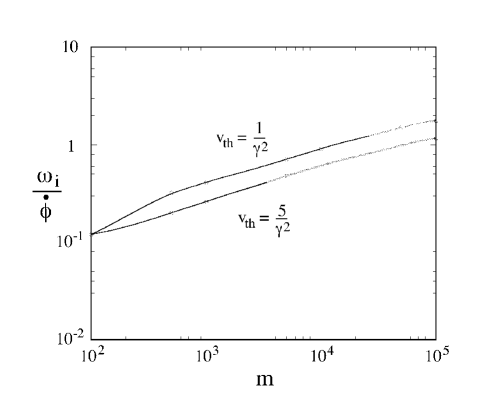
Figure 7: Solutions of the dispersion relation in the presence of betatron oscillations in the limit $\bar{k}_{r}v_{th}\ll 1$, $\gamma=30$, $\zeta=0.02$. Points which do not satisfy the inequalities $m\gg 1$, $m^{2/3}v_{th}<1$ and $|\Delta\tilde{\omega}|^{2}<F_{0}v_{th}^{2}$ are plotted in gray.

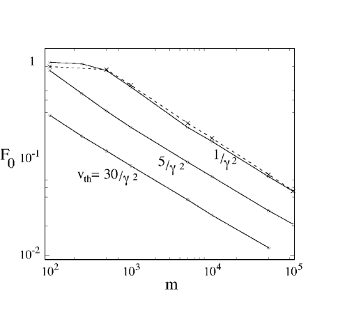
Figure 8: $F_{0}$ as a function of $m$ for $\gamma=30$, $\zeta=0.02$ and various $v_{th}$ and the squared ratio of the growth rates from Fig. 2 and Fig. 7 (dash-triple-dotted)

We could also study the effect of the non-zero thickness alone without betatron oscillations setting $F_{0}=1$ and $F_{n\neq 0}=0$ and solving the full eigenvalue problem. Due to the complicated nature of the dispersion relation we have not done this yet. Note that the thin approximation will suppress certain modes, e.g. the negative mass instability cannot be expected to be present with the fields having been evaluated at one radius only, cf. Briggs1966 .

VIII Spectrum of Coherent Radiation

Having computed the growth rate and the saturation amplitude, the radiated power can now be calculated. Starting from Eq. (106) we now have

$$P_{m}={\pi\over 2}L\omega r_{0}^{4}~{}\big{|}\delta J_{\phi 0}\big{|}^{2}\left|\int\xi d\xi e^{i\bar{k}_{r}\xi}J_{m}^{\prime}(\omega r_{0}\xi)\right|^{2}~{},$$ (91)

where $\xi\equiv r/r_{0}$ and the integration is over the thickness of the layer. The Bessel function can be expressed approximately in term of an Airy function as done before. We take the linear approximation to the Airy function as discussed previously, and this gives

$$P_{m}=\frac{\pi L\omega}{2}r_{0}^{4}c_{2}^{2}\left(\frac{2}{m}\right)^{4/3}\big{|}\delta J_{\phi 0}\big{|}^{2}\left|\int_{1-v_{th}}^{1+v_{th}}\xi d\xi e^{i\bar{k}_{r}\xi}\right|^{2}~{},$$ (92)

where $c_{2}\approx 0.259$. This is valid for sufficiently big values of $\gamma$ and low $m$. The largest values occur for $\bar{k}_{r}v_{th}\ll 1$, where this quantity is simply $4v_{th}^{2}$. This is enough motivation for us to work in this limit. Thus,

$$P_{m}\leq 2\pi L\omega r_{0}^{4}c_{2}^{2}v_{th}^{2}\left|\delta J_{\phi 0}\right|^{2}\left(\frac{2}{m}\right)^{4/3}~{}.$$ (93)

Because we calculated our growth rates in the thin approximation for $k\approx k_{\phi}$ it is consistent to use $\delta\phi=4\pi^{2}v_{th}v_{\phi}^{-1}Zr_{0}\delta J_{\phi 0}$. Furthermore, we set $\omega\rightarrow m\dot{\phi}$. This is consistent even for large growth rates since the exponential growth has stopped. With our expression for the saturation amplitude we obtain

$$P_{m}\leq\frac{Lc_{2}^{2}v_{\phi}^{2}m_{e}^{2}}{8\pi^{3}r_{0}e^{2}}\frac{\gamma^{6}}{|Z|^{2}}\left(\frac{2}{m}\right)^{4/3}{1\over m^{3}}\left(\frac{\omega_{i}(m)}{\dot{\phi}}\right)^{4}~{}.$$ (94)

Since the number of particles $N$ is proportional to $\zeta$ and the growth rates are proportional to $\sqrt{\zeta}$ for $m>m_{1}$ the radiated power scales like $N^{2}$. This suggests that the emitted radiation is coherent. In Fig. 9 we plotted the radiated power in arbitrary units having evaluated $F_{0}$ numerically. For large $m$ the curve scales as $m^{-5/3}$. Analytically we obtain with our second approximation for $F_{0}$ the scaling $m^{-3}(m^{2/3}/m^{1/4})^{4}=m^{-4/3}$. With $|Z|^{2}\approx 4c_{1}^{4}\left({2}/{m}\right)^{4/3}$ we obtain

$$P_{m}\lesssim 3.71\times 10^{14}\gamma^{6}m^{-3}\frac{L}{r_{0}}\left(\frac{\omega_{i}}{\dot{\phi}}\right)^{4}\frac{\rm erg}{\rm s}~{}.$$ (95)

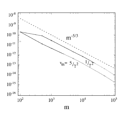
Figure 9: Radiated power $(m^{-3}(\omega_{i}/\dot{\phi})^{4})$ for $\gamma=30$ and $\zeta=0.02$ in arbitrary units. The straight line is proportional to $m^{-5/3}$ and is shown for comparison. Points which do not satisfy the inequalities $m\gg 1$, $m^{2/3}v_{th}<1$ and $|\Delta\tilde{\omega}|^{2}<F_{0}v_{th}^{2}$ are plotted in gray.

VIII.1 Brightness Temperatures

We consider the brightness temperatures $T_{B}$ for conditions relevant to the radio emissions of pulsars. Using the Rayleigh-Jeans formula $B_{\nu}=2k_{B}T_{B}(\nu/c)^{2}$ for the radiated power per unit area per sterradian at a frequency $\nu=m\dot{\phi}/2\pi$ gives

$$2k_{B}T_{B}({\nu/c})^{2}{\cal A}\Delta\Omega=2\pi P_{m}/\dot{\phi}$$

$$T_{B}\lesssim 4.5\times 10^{21}\frac{\rm K}{\rm m}\cdot L\gamma^{6}m^{-4}\left(\frac{\omega_{i}}{\dot{\phi}}\right)^{4}$$ (96)

where $k_{B}$ is Boltzmann’s constant and ${\cal A}=2\pi r_{0}L$ is the area of the E-layer. The solid angle of the source seen by a distant observer has been computed in appendix A and its value is $\Delta\Omega={4\pi^{2}r_{0}}/({mL})$. It is assumed that the angular size of the source is small such that that radiation from the top and the bottom emitted at an angle $\theta$ with respect to the normal is received by the observer at the same position. For the sample values $\gamma=1000$, $\zeta=0.08$, $v_{th}=0.04\gamma^{-2}$, $L=100$ km and $m=m_{1}$ our model predicts a maximum brightness temperature of $T_{B}\approx 2\times 10^{20}{\rm K}$. According to our results from previous sections there may be degeneracy from modes with non-zero axial wavenumbers $k_{z}$. It is reasonable to assume that this will increase the brightness temperature by a factor in the order of $m\tan\psi_{cr}$. Beaming along the z-axis may increase the brightness temperature and the observed frequency even further.

IX Applications in Accelerator Physics

The next-generation linear collider requires a beam with very short bunches and low emittance. That is, the beam must occupy a very small volume in phase space. The emittance of the pre-accelerated beam is reduced in a damping ring which is operated with longer bunches to avoid certain instabilities. The bunch length has to be decreased in a so-called bunch compressor before the beam can be injected into the linear collider. A bunch compressor consists of an accelerating part and an arc section. Since the bunch lengths of the proposed linear colliders are in the order of the wavelength of the synchrotron radiation which is being radiated in the arc section, instabilities due to coherent synchrotron have to be taken seriously. For a design energy of $2$ GeV and $7\times 10^{11}$ electrons per 100 $\mu$m our dimensionless quantities become $\gamma=4000$ and $\zeta=0.08$ Raubenheimer . Our qualitative analysis of the betatron motion suggests that CSR is suppressed for a minimum energy spread of $v_{th}>\zeta^{-1}\gamma^{-2}=12.5\gamma^{-2}$.

X Discussion and Conclusions

This work has studied the stability of a collisionless, relativistic, finite-strength, cylindrical electron (or positron) layer by solving the Vlasov and Maxwell equations. This system is of interest to understanding the high brightness temperature coherent synchrotron radio emission of pulsars and the coherent synchrotron radiation observed in particle accelerators. The considered equilibrium layers have a finite ‘temperature’ and therefore a finite radial thickness. The electrons are considered to move either almost perpendicular to a uniform external magnetic field or almost parallel to an external toroidal magnetic field. A short wavelength instability is found which causes an exponential growth an initial perturbation of the charge and current densities. The periodicity of these enhancements can lead to coherent emission of synchrotron radiation. Neglecting betatron oscillations we obtain an expression for the growth rate which is similar to the one found by Goldreich and Keeley Goldreich & Keeley (1971) if the thermal energy spread is sufficiently small. The growth rate increases monotonically approximately as $m^{1/2}$, where $m$ is the azimuthal mode number which is proportional to the frequency of the radiation. With the radial betatron oscillations included, the growth rate varies as $m^{1/3}$ over a significant range before it begins to decrease.

We argue that the growth of the unstable perturbation saturates when the trapping frequency of electrons in the wave becomes comparable to the growth rate. Owing to this saturation we can predict the radiation spectrum for a given set of parameters. For the realistic case including radial betatron oscillations we find a radiation spectrum proportional to $m^{-5/3}$. This result is in rough agreement with observations of radio pulsars Manchester & Taylor (1977). The power is also proportional to the square of the number of particles which indicates that the radiation is coherent. Numerical simulations of electron rings based on the fully relativistic, electromagnetic particle-in-cell code OOPIC schmekel2004b recovers the main scalings found here.

*

Appendix A Green’s Function

The Green’s function for the potentials give

$$\delta\Phi({\bf r},t)=\int dt^{\prime}d^{3}r^{\prime}~{}G({\bf r}-{\bf r^{\prime}},t-t^{\prime})~{}\delta\rho({\bf r}^{\prime},t^{\prime})~{}.$$

$$\delta{\bf A}({\bf r},t)=\int dt^{\prime}d^{3}r^{\prime}~{}G({\bf r}-{\bf r^{\prime}},t-t^{\prime})~{}\delta{\bf J}({\bf r}^{\prime},t^{\prime})~{},$$ (97)

where

$$\left(\nabla^{2}-{\partial^{2}\over\partial t^{2}}\right)G({\bf r},t)=-4\pi\delta(t)\delta({\bf r})~{},~{}~{}\tilde{G}({\bf k},\omega)={4\pi\over{\bf k}^{2}-\omega^{2}}~{},$$

$$G({\bf r},t)=\frac{4\pi}{(2\pi)^{4}}\int_{C}d\omega\int d^{3}k~{}{\exp(i{\bf k\cdot r}-i\omega t)\over{\bf k}^{2}-\omega^{2}}~{},$$ (98)

where $\tilde{G}$ is the Fourier transform of the Green’s function. The “C” on the integral indicates an $\omega-$integration parallel to but above the real axis, ${\rm Im}(\omega)>0$, so as to give the retarded Green’s function.

Because of the assumed dependences of Eq. (26), we have for the electric potential,

$$\delta\Phi_{\omega mk_{z}}(r)=2\int_{0}^{\infty}r^{\prime}dr^{\prime}\int_{0}^{\infty}\kappa d\kappa\int_{0}^{2\pi}d\alpha~{}~{}\delta\rho_{\omega mk_{z}}(r^{\prime})\big{[}..\big{]}$$

$$=4\pi\int_{0}^{\infty}r^{\prime}dr^{\prime}\int_{0}^{\infty}\kappa d\kappa~{}{J_{m}(\kappa r)J_{m}(\kappa r^{\prime})\over\kappa^{2}-(\omega^{2}-k_{z}^{2})}~{}\delta\rho_{\omega mk_{z}}(r^{\prime})~{},$$ (99)

where

$$\big{[}..\big{]}\equiv{\exp(im\alpha)J_{0}\{\kappa[r^{2}+(r^{\prime})^{2}-2rr^{\prime}\cos\alpha]^{1/2}\}\over\kappa^{2}-(\omega^{2}-k_{z}^{2})}~{},$$

where $\kappa^{2}\equiv k_{x}^{2}+k_{y}^{2}$. Because $\omega$ has a positive imaginary part, this solution corresponds to the retarded field. Also because ${\rm Im}(\omega)>0$, the $\kappa-$integration can be done by a contour integration as discussed in Watson (1966) which gives

$$\delta\Phi_{\omega mk_{z}}(r)\!=\!2\pi^{2}i\int_{0}^{\infty}\!\!\!r^{\prime}dr^{\prime}J_{m}(kr_{<})H_{m}^{(1)}(kr_{>})\delta\rho_{\omega mk_{z}}(r^{\prime}),$$ (100)

where $k\equiv(\omega^{2}-k_{z}^{2})^{1/2}$, where $r_{<}$ ($r_{>}$) is the lesser (greater) of $(r,r^{\prime})$, and where $H_{m}^{(1)}(x)=J_{m}(x)+iY_{m}(x)$ is the Hankel function of the first kind. From the Lorentz gauge condition

$$\delta\Psi^{\omega mk_{z}}(r)=r\delta A_{\phi}^{\omega mk_{z}}=r_{0}v_{\phi}\left(1+\Delta\tilde{\omega}\right)\delta\Phi^{\omega mk_{z}}(r)$$ (101)

Equations (100) and (101) are useful in subsequent calculations.

To determine the total synchrotron radiation from the E-layer it is sufficient to calculate $\delta{\bf A}$ at a large distance from the E-layer. We assume that the E-layer has a finite axial length and exists between $-L/2\leq z\leq L/2$. Thus we evaluate $\delta{\bf A}$ in a spherical coordinate system ${\bf R}=(R,\theta,\phi)$ at a distance $R\gg L$. The retarded solution is

$$\delta{\bf A}({\bf R})={1\over R}\int d^{3}r^{\prime}~{}\delta{\bf J}\bigg{(}{\bf r}^{\prime},t-|{\bf R}-{\bf r}^{\prime}|\bigg{)}=$$

$${\exp(i\omega R)\over R}\int\!\!\!d^{3}r^{\prime}~{}\delta{\bf J}(r^{\prime})\exp\bigg{[}im\phi^{\prime}+ik_{z}z^{\prime}-i\omega(t+\hat{\bf R}\cdot{\bf r}^{\prime})\bigg{]},$$ (102)

(see, e.g. ch. 9 of Landau & Lifshitz (1962)). The source point is at $(x^{\prime}=r^{\prime}\cos\phi^{\prime},~{}y^{\prime}=r^{\prime}\sin\phi^{\prime},~{}z^{\prime})$. The observation point is taken to be at $(x=0,~{}y=R\sin\theta,~{}z=R\cos\theta)$. Consequently, $\hat{\bf R}\cdot{\bf r}^{\prime}=r^{\prime}\sin\theta\sin\phi^{\prime}+z^{\prime}\cos\theta$. The phase factor $\exp(i\omega R)$ does not affect the radiated power and is henceforth dropped.

For the cases where $\delta J_{\phi}$ is the dominant component of the current-density perturbation we have

$$\bigg{[}\delta A_{x}^{\omega},~{}\delta A_{y}^{\omega}\bigg{]}={S(\theta)\over R}\int r^{\prime}dr^{\prime}d\phi^{\prime}~{}\bigg{[}-\sin\phi^{\prime},\cos\phi^{\prime}\bigg{]}\times$$

$$\delta J_{\phi}(r^{\prime})~{}\exp(im\phi^{\prime}-i\omega r^{\prime}\sin\theta\sin\phi^{\prime})~{},$$ (103)

where

$$S(\theta)\equiv L~{}{\sin[(k_{z}-\omega\cos\theta)L/2]\over(k_{z}-\omega\cos\theta)L/2}$$ (104)

is a structure function accounting for the finite axial length of the E-layer, and $\omega$ superscript indicates $\omega=m\dot{\phi}$. Carrying out the $\phi^{\prime}$ integration in equation (103) gives

$$\bigg{[}\delta A_{x}^{\omega},~{}\delta A_{y}^{\omega}\bigg{]}={S(\theta)\over R}\int r^{\prime}dr^{\prime}~{}\delta J_{\phi}(r^{\prime})\big{[}..\big{]}$$ (105)

where

$$\big{[}..\big{]}\equiv\left[iJ_{m}^{\prime}(\omega r^{\prime}\sin\theta),~{}{m\over\omega r^{\prime}\sin\theta}J_{m}(\omega r^{\prime}\sin\theta)\right]$$

and where the prime on the Bessel function indicates its derivative with respect to its argument. The radiated power per unit solid angle is

$${dP_{\omega}\over d\Omega}={R^{2}\over 8\pi}|\delta{\bf B}^{\omega}|^{2}={R^{2}\over 8\pi}|{\bf k}\times\delta{\bf A}^{\omega}|^{2}=$$

$${R^{2}\omega^{2}\over 8\pi}\left(|\delta A_{x}^{\omega}|^{2}+\cos^{2}\theta|\delta A_{y}^{\omega}|^{2}\right)~{},$$ (106)

where ${\bf k}\equiv\omega\hat{\bf R}$ is the far field wavevector.

For a radially thin E-layer, $(\Delta r/r_{0})^{2}\ll 1$, equations (105) and (106) give

$${dP_{\omega}\over d\Omega}={S^{2}(\theta)\over 8\pi}\left|\int r^{\prime}dr^{\prime}~{}\delta J_{\phi}(r^{\prime})\omega J_{m}^{\prime}(\omega r_{0}\sin\theta)\right|^{2}+$$

$${S^{2}(\theta)\over 8\pi}\left|\int r^{\prime}dr^{\prime}~{}\delta J_{\phi}(r^{\prime}){m~{}{\rm cot}~{}\theta\over r_{0}}J_{m}(\omega r_{0}\sin\theta)\right|^{2}~{}.$$ (107)

The factor within the curly brackets is the same as that for the radiation pattern of a single charged particle (see ch. 9 of Landau & Lifshitz (1962)).

The factor $S^{2}(\theta)$ in Eq. (107) tightly constrains the radiation to be in the direction $\theta_{*}=\cos^{-1}(k_{z}/\omega)$ if the angular width of $S^{2}(\theta)$, the half-power half-width $\Delta\theta_{1/2}\approx\pi/(\omega L)$, is small compared with the angular spread of the single particle synchrotron radiation, $1/\gamma$, which is the angular width due to the Bessel function terms in Eq. (107). This corresponds to E-layers with $L\gg\pi\gamma/\omega=\pi r_{0}\gamma/m$. For $L\sim r_{0}$, we need $m\gg\pi\gamma$, which is satisfied by the spectra discussed later in §8. In this case, Eq. (107) can be integrated over the solid angle to give

$$P_{\omega}={\pi L\sin\theta_{*}\over 2\omega}\left\{\left|\int r^{\prime}dr^{\prime}~{}\delta J_{\phi}(r^{\prime})\omega J_{m}^{\prime}(\omega r_{0}\sin\theta_{*})\right|^{2}+\right.$$

$$\left.\left|\int r^{\prime}dr^{\prime}~{}\delta J_{\phi}(r^{\prime}){m~{}{\rm cot}~{}\theta_{*}\over r_{0}}J_{m}(\omega r_{0}\sin\theta_{*})\right|^{2}\right\}~{}.$$ (108)

One limit of interest of Eq. 108 is that where $k_{z}=0$ so that $\theta_{*}=\pi/2$ and

$$P_{m}={\pi mv_{\phi}L\over 2r_{0}}\left|\int r^{\prime}dr^{\prime}~{}\delta J_{\phi}(r^{\prime})J_{m}^{\prime}(\omega r_{0})\right|^{2}~{},$$ (109)

where we have set $\omega\rightarrow m\dot{\phi}$. The total radiated power is $P=\sum_{m}P_{m}$.