The Baryonic Tully-Fisher relation revisited

The Baryonic Tully-Fisher relation (BTF) can be substantially improved when considering that the galactic baryonic mass is likely to consist not only of the detected baryons, stars and gas, but also of a dark baryonic component proportional to the HI gas. The BTF relation is optimally improved when the HI mass is multiplied by a factor of about 3, but larger factors up to $11-16$ still improve the fit over the original one using only the detected baryons. The strength of this improved relation is quantified with up-to-date statistical tests such as the Akaike Information Criterion or the Bayesian Information Criterion. In particular they allow us to show that supposing a variable $M_{\star}/L$ ratio instead is much less significant. This result reinforces the suggestion made in several recent works that mass within galactic disks must be a multiple of the HI mass, and that galactic disks are substantially, but not necessarily fully, self-gravitating.

1 Introduction

McGaugh et al. (2001) (hereafter MSBD) have extended the Tully-Fisher relation (Tully & Fisher 1977) (TF) over 5 dex in stellar mass and 1 dex in velocity by correlating not the luminosity with the rotation velocity, but the detected baryon mass with the rotation velocity. This is an important step toward understanding the TF relation, because the physical causality link between mass and rotational velocity, gravitational dynamics, is much more direct than between stellar light production and rotational velocity. The traditional TF relation requires us to understand how the nuclear energy production inside stars may well be tightly correlated with the global rotation speed of the galaxy, while the baryonic TF (BTF) just requires finding the link between the baryonic mass and kinematics.

The baryons considered by MSBD include the stars, the total mass of which is inferred from a plausible stellar mass to light ratio, and neutral hydrogen HI from 21 cm measurements, including a cosmic helium fraction. Doing so, MSBD show with a sample of 243 galaxies that a scatter plot of velocity–mass looks straighter when summing the HI mass to the stellar mass. The argument advanced by MSBD is that a better relation exists between these baryons and rotational velocity than between light and rotational velocity because the low surface brightness galaxies in the sample have a very low stellar mass content. This makes sense because in the limit of a pure gaseous protogalactic disk no stars shine, yet the disk does rotate.

Several reasons motivated us to reexamine this work. By naming the improved relation “baryonic” MSBD implies that the baryons are well represented by the detected stars and HI, while in many spirals often as much gas as the detected HI but in the form of H₂ can be inferred from CO observations with the conventional proportionality $X$ factor between the CO emission and the H₂ mass (Combes 2004). This point is however not necessarily crucial because the CO emission is often roughly located in the optical disk, so the CO related H₂ mass may be well absorbed, to a first approximation, in the mass to light ratio of the stellar mass. But for years now the universality of the $X$ factor has been challenged. Recent rediscussions of this factor (e.g., Boulanger 2004) favor an increased $X$ in low metallicity, low excitation or cold conditions, typical of outer galactic HI disks, by at least one order of magnitude.

Long ago Bosma (1981a) pointed out that the dynamical mass in spirals is known to be well correlated to a multiple of the detected HI (see also Hoekstra et al. 2001). So a natural hypothesis reinforced by a series of arguments presented in Pfenniger, Combes & Martinet (1994), and Pfenniger & Combes (1994) as well as variants discussed by other authors (Henriksen & Widrow 1995; de Paolis et al. 1995; Gerhard & Silk 1996) is to assume that a sufficiently cold form of H₂ can well make up a sizable fraction of the unseen baryonic mass in the disk. Moreover, several new theoretical and observational arguments indicate that galactic disks may be more massive than usually thought. Kalberla (2003) found that the mass distribution and the dynamics of the Milky Way is dominated by a dark matter disk. Massive disks are also needed to explain spiral structures in low surface brightness galaxies (Fuchs 2003; Mayer & Wadsley 2004), as well as in extended HI disks like in the blue compact dwarf galaxy NGC 2915 (Masset & Bureau 2003). In the context of warped galaxies, Revaz & Pfenniger (2004) have recently shown that the high number of warped spirals results naturally from bending instabilities, if the disk contributes to at least $60$% of the total galactic mass, within $30\,\rm{kpc}$.

The true number of baryons contained in spiral galaxies can still be a multiple of the detected ones. Presently the hypothesis that MACHOS can represent an important part of the unseen baryonic mass in an extended halo seems to be disproved by the micro-lensing experiments towards the Magellanic clouds and the Galactic center (Alcock et al. 2001; Afonso et al. 2003), but a dark baryonic component closer to the outer disk, i.e., more closely related to the HI distribution, has not been investigated to a similar extent yet.

If some sizable fraction of the mass correlates well with velocity, and the detected baryons within the radius of measured velocities do represent a non-negligible amount of the total mass within this radius, it seems reasonable to check whether the full dynamical mass could not improve the correlation. Indeed, gravitational dynamics is little dependent on the nature of matter over a few dynamical time-scales.

In order to investigate better the underlying apparent correlation, the analysis of the MSBD sample can easily be extended by up-to-date statistical tools. Below, we use statistical tools, mainly the Akaike Information Criterion (Akaike 1974), and the Bayesian Information Criterion (Schwarz 1978) that are not well known in astronomy, but have been often used in many other scientific fields over the last two decades. They provide interesting decision criterions for discriminating quantitatively between models using a different number of fitting parameters for the same data set. The curious reader will find in Liddle (2004) a short introduction for astronomers to these methods, and an application to the cosmological parameters.

The purpose of the following Sections is therefore to extend the discussion about the BTF with more advanced statistical techniques than the ones currently popular in astronomy.

2 Sample

MSBD kindly provided us the sample that they used in their work, and to make a reasonable comparison we use here exactly the same sample, including the same assumptions about the mass-to-light ratios of the stellar and HI components. The sample consists of 243 approximately face-on spirals with peak rotational velocities in the range 33 to $323\,\rm km\,s^{-1}$, almost a dex. For a more detailed description of the sample we refer the reader to the MSBD paper.

3 Optimized HI scaling

3.1 Full sample

The first question is how scaling HI with a constant factor $c$ different from $1$ changes the fit rms. Using a linear least-squares fit, for $c$ in the range $[0-15]$, we calculate the corresponding coefficients $a$ and $b$ in the least-squares relation linking the stellar mass $M_{\star}$ inferred from the light and a constant $M_{\star}/L$ ratio, the HI mass $M_{\rm HI}$, and the rotational velocity $V_{\rm c}$:

$$\log(M_{\star}+cM_{\rm HI})\approx a+b\log V_{\rm{c}}\,,$$ (1)

as well as the rms of the respective fits as a function of $c$, which are plotted in Fig. 1. Clearly, passing from $c=0$ ($\rm{rms}=0.521$) in the usual TF relation to $c=1$ ($\rm{rms}=0.329$) in the BTF relation decreases the fit rms by a factor of $1.6$, which is the main new point in MSBD’s paper. Yet the curve rms($c$) continues to decrease for $c>1$ down to a shallow minimum at $c=2.98$ ($\rm{rms}=0.3164$). Beyond this optimal $c$, the rms grows slowly, such that up to $c=11.5$ the rms fit is still better than for $c=1$.

Figure 1: Rms of the linear least-squares fit as a function of the parameter $c$ (see Eq. 1). The dotted line indicates MSBD’s rms value ($c=1$).

Fig. 2 shows the least-squares fit of the extended BTF (hereafter EBTF) relation at the optimal value $c_{\rm opt}=2.98$, where the linear fit parameters are $a=3.11$ and $b=3.36$.

Figure 2: Least-squares fit of the Baryonic Tully-Fisher relation using Eq. 1 with $a=3.11$, $b=3.36$ and $c=2.98$.

3.2 Comparing models

With an additional parameter, we naturally expect that the rms of the EBTF model (Eq. 1) decreases with respect to the simpler BTF model (null hypothesis), where $c$ remains fixed to $1$. Thus, even if the rms is lower, it does not mean that the data are better fitted by the EBTF model.

To test this, we have used three different statistical tools. The first tool is classical, while the two more recent ones are less well known in astronomy, but have become popular elsewhere. The methods work under the assumption that the error distribution is Gaussian. A study of the rms distribution shows that the data points do verify reasonably well this assumption.

3.2.1 Extra sum-of-squares $F$-Test

This standard test consists of comparing the difference between the $\chi 2$ sums of two models, say model 1 and model 2, where model 1 is a simpler case of model 2 . Because model 1 has a lower number of parameters, we usually expect that $\chi 2_{1}$ is greater than $\chi 2_{2}$ with a difference corresponding to the difference $r$ of parameters between the two models. Thus, the ratio $\left(\chi 2_{1}-\chi 2_{2}\right)/r$ provides an estimate of the goodness of one model compared to the other. An $F$-value is defined by dividing the previous ratio by the normalised fraction $\chi 2_{2}/(N-k_{2})$, where $N-k_{2}$ is the degrees of freedom of model 2 with $k_{2}$, its number of parameters. Explicitly, $F$ is written as:

$$F=\frac{\left(\chi 2_{1}-\chi 2_{2}\right)}{r}\,\Bigg{/}\,\frac{\chi 2_{2}}{(N-k_{2})}\,.$$ (2)

Since $F$ is a ratio of two $\chi 2$ distributions, it follows an $F$-distribution. We can then compute the probability $P$ to find a value greater than $F$ for such a distribution. If this probability is weak (typically less than 5%), we can conclude that the $F$-value obtained has a weak probability to result from the error fluctuations and that the data is significantly better fitted by model 2.

Assuming that the intrinsic errors $\sigma_{i}$ are constant for each point $i$ ($\sigma_{i}=\sigma$), the $\chi 2$ terms in Eq. (2) can be replaced by the sum-of-squares $S2_{i}$:

$${S2_{i}}=\sum_{j=1}^{N}\left(y_{j}-f_{i}(x_{j})\right)2\,,$$ (3)

where the $y_{j}$ correspond to the left hand side of Eq. (1) and the $f_{i}(x_{j})$ to the right hand one. A rigorous description of this classical test can be found, e.g., in Lupton (1995, p. 98-101).

Comparing the EBTF model with the simpler BTF model, with $N=243$, $k_{1}=2$ and $r=1$, we obtain $F=19.9$, to which the associated probability $P$ is lower than $0.01$%, which is the probability for the BTF model to be better than the EBTF one.

3.2.2 Akaike’s Information Criterion corrected (AICc)

The second performed test is derived form the Information theory, namely the Akaike’s Information Criterion corrected (AICc) (Sakamoto, Ishiguro & Kitagawa 1986; Burnham & Anderson 2004). Since the formal derivation of this test is somewhat lengthy we refer the reader to the literature for more details (see, e.g., Brockwell & Davis 2002; Burnham & Anderson 2004). However, its application is as simple as the Extra sum-of-squares $F$-Test, without the need to introduce additional assumptions. The AICc consists of computing for the two models the values:

$$\mathcal{A}^{\rm c}_{i}=N\,\ln\left(\frac{S2_{i}}{N}\right)+2\,k_{i}+\frac{2\,k_{i}\left(k_{i}+1\right)}{N-k_{i}-1}\,,$$ (4)

where $k_{i}$ is the number of parameters of model $i$ and $S2_{i}$ is the corresponding sum-of-squares defined by Eq. (3). In this formula, the first term is the entropy term, which usually decreases when the number of parameters $k_{i}$ increases. It is balanced by the second term linear in $k_{i}$. The third term is the correction term especially relevant when $N$ is small, so unimportant here. As for entropy in statistical mechanics, the value of $\mathcal{A}^{\rm c}_{i}$ depends on the choice of data unit, therefore its value has no absolute meaning, only the difference between two models has one: the relative information content. The best model is simply the one with the lowest $\mathcal{A}^{\rm c}_{i}$ value, where the decrease of the entropy term dominates. The difference $\Delta\mathcal{A}^{\rm{c}}=\mathcal{A}^{\rm{c}}_{2}-\mathcal{A}^{\rm{c}}_{1}$ allows us to quantify how much a model is better than another. The probability $\mathcal{P}_{2,1}$ that model 2 is better than model 1 is given by:

$$\mathcal{P}_{2,1}=\frac{e^{-\frac{1}{2}\,\Delta\mathcal{A}^{\rm{c}}}}{1+e^{-\frac{1}{2}\,\Delta\mathcal{A}^{\rm{c}}}}.$$ (5)

The comparison of the BTF model with the EBTF one gives respectively $\mathcal{A}^{\rm{c}}_{1}=-533.79$ and $\mathcal{A}^{\rm{c}}_{2}=-551.14$. The so called “information ratio” $\mathcal{P}_{2,1}/\mathcal{P}_{1,2}$ tells us that the EBTF model is 5854 times more likely to be correct than the BTF one.

3.2.3 Bayesian Information Criterion (BIC)

Another criterion which is often less favorable for models with many parameters is the Bayesian Information Criterion (BIC) (Schwarz 1978). This criterion, favoured by Liddle (2004), weights more heavily additional model parameters than AICc for data sets with large $N$. As AICc, BIC does not require us to compare nested models. The BIC consists of computing for two models the values:

$$\mathcal{B}_{i}=N\,\ln\left(\frac{S2_{i}}{N}\right)+k_{i}\ln N\,,$$ (6)

where the parameters have the same meaning as before. As for AICc, only the difference of $\mathcal{B}_{i}$ is important, not their particular value.

The comparison of the BTF model with the EBTF one gives respectively $\mathcal{B}_{1}=-523.41$ and $\mathcal{B}_{2}=-537.34$. Applying the analogue of Eq. (5) for BIC yields that the EBTF model is 1054 times more likely to be correct than the BTF one.

3.2.4 Comparison with a quadratic fit

In order to convince ourself of the strength of the three previous comparison methods, we have compared the BTF model with a third model, where the data is simply fitted with a quadratic function, therefore with the same number of free parameters ($k=3$) as our model:

$$\log(M_{\star}+M_{\rm HI})\approx a+b\log V_{\rm{c}}+c^{\prime}\log 2V_{\rm{c}}\,.$$ (7)

Comparing this quadratic model with the BTF model, the $F$-test gives a probability $P$ of only $37.9$%. In this case, the weak decrease of the rms of the more complex model is not sufficient to justify the additional parameter $c^{\prime}$. The AICc $\mathcal{A}^{\rm c}_{i}$ for the two models are respectively $-533.79$ and $-532.51$; the BIC $\mathcal{B}_{i}$, $-523.41$ and $-518.70$ respectively: the BTF model is clearly a slightly better model than the quadratic fit.

Since a quadratic model does not significantly improve the fit, we can then conclude that the improvement reached by the EBTF model does not result merely from the additional parameters but rather from the judicious choice of the fitting law Eq. (1), directly inspired by physical considerations.

3.3 Subsamples

In this Section, we check the robustness of the result obtained in Sect. 3 when removing points from the the MSBD data. All the subsamples containing all but one or two points are analysed.

Figure 3: Bottom: Histogram of the optimal $c_{\rm opt}$ values obtained by fitting Eq. (1) to successively the 243 distinct subsamples made of 242 data points. Top: Rms of each subsample fit.

For each of the $N=243$ subsamples, where in each one a single point has been successively removed, we have computed the optimal $c_{\rm{opt}}$ value, as described in Sect. 3.1. The histogram of those values is displayed at the bottom of Fig. 3. The values $c_{\rm{opt}}$ lie in the interval $2.65$ and $3.24$ with a mean of $2.98$ and a dispersion of $0.05$. Therefore the optimal $c_{\rm{opt}}$ is little sensitive to the error produced by any single data point.

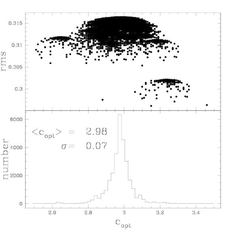
Figure 4: Bottom: Histogram of the optimal $c_{\rm{opt}}$ values obtained by fitting Eq. (1) to each of the distinct 29403 subsamples made of 241 data points. Top: Rms of each subsample fit.

The same exercise is repeated by successively removing two different points for each distinct combination allowed by 243 data points. Thus, $243\times 242/2=29403$ searches for an optimal value of $c_{\rm{opt}}$ have been computed. The found $c_{\rm{opt}}$ range between $2.51$ and $3.46$ with a mean of $2.98$ and a dispersion of $0.07$.

In the rms of both histogram peaks, we observe that a particular removed point contributes to a particularly large decrease of the rms and an increase of $c_{\rm opt}$. This point corresponds to the isolated lower left point of Fig. 2. It is important to emphasize that the conclusions obtained in the previous Section are not lessened by this point. On the contrary, removing it increases significantly the goodness of the EBTF model with respect to the BTF one.

3.4 Independent sample

In order to check the dependence of the previous results on MSBD’s particular sample, we have repeated the analysis of Sect. 3.2 on another independent sample. We have chosen the sample proposed by Sanders & McGaugh (2002) that contains 76 galaxies, where the luminosities (in either B, R, K or H bands) as well as the HI mass are provided. Among those galaxies, we have removed 29 of them that are contained in MSBD’s data. They correspond to the UMa sample of Verheijen (2001). The average mass-to-light ratio for each band has been chosen according to MSBD. For the R band, the missing value has been interpolated and set to 1.2. The rms of the data fit of Eq. 1 as a function of $c$ is displayed in Fig. 5. The found optimal value $c_{\rm{opt}}=3.42$ ($\rm{rms}=0.256$) is slightly higher than for MSBD’s sample. Beyond this value, the rms grows slowly up to $c=16.5$ where it is still better than for $c=1$ ($\rm{rms}=0.275$).

Figure 5: Rms of the linear least-squares fit as a function of the parameter $c$ (see Eq. 1), for the sub-sample of Sanders & McGaugh (2002). The dotted line indicates the rms value for $c=1$.

The results of the extra sum-of-squares $F$-Test, AICc and BIC tests are displayed in Table 1. Those tests compare the BTF fit with the EBTF one and with the quadratic fit of Eq. (7).

BTF vs EBTF	BTF vs “quadratic”
$F$-Test
$F=6.81$	$F=2.03$
$P=1.24$ %	$P=16$ %
AICc
$\mathcal{A}^{\rm{c}}_{1}=-114.72$	$\mathcal{A}^{\rm{c}}_{1}=-114.72$
$\mathcal{A}^{\rm{c}}_{2}=-119.08$	$\mathcal{A}^{\rm{c}}_{2}=-114.44$
$\mathcal{P}_{2,1}/\mathcal{P}_{1,2}=8.8$	$\mathcal{P}_{2,1}/\mathcal{P}_{1,2}=0.87$
BIC
$\mathcal{B}_{1}=-109.72$	$\mathcal{B}_{1}=-109.72$
$\mathcal{B}_{2}=-112.63$	$\mathcal{B}_{2}=-107.99$
$\mathcal{P}_{2,1}/\mathcal{P}_{1,2}=4.2$	$\mathcal{P}_{2,1}/\mathcal{P}_{1,2}=0.42$

Table 1: Statistical comparison of the BTF model with the EBTF one, and with the quadratic model, for Sanders & McGaugh sub-sample data.

While the trend is slightly less pronounced in this new but smaller sample, the statistical tests confirm that the EBTF model is better than the BTF one ($4$ to $9$ times). The choice of Eq. (1) is again supported by the fact that the quadratic model (with the same number of parameters than the EBTF one) does not improve the fit.

3.5 Variable $M_{\star}/L$

A questionable assumption included in the stellar mass derivation in MSBD’s sample is that the stellar $M_{\star}/L$ ratio is taken as constant, while in a sample of spirals it can typically vary by a factor of several, more in B than in the NIR bands.

However, along the spiral sequence the rotational velocity is known to correlate with the stellar $M_{\star}/L$ ratio: small late type spirals typically rotate slower and are bluer (so have a lower stellar $M_{\star}/L$ ratio) than massive and fast rotating late spirals. As an illustration, in Broeils’ sample (1992), the $M_{\star}/L_{\rm B}$ ratio of 23 bright galaxies spanning the spiral sequence can be reasonably represented by a linear regression:

$${M_{\star}\over L_{\rm B}}=4.00\log V_{\rm max}-5.77\,.$$ (8)

Supposing now that instead of a constant $M_{\star}/L$ ratio, one would include the above more accurate statistical knowledge in the EBTF. The former constant $M_{\star}/L$ in MSBD data for each galaxy would be replaced by a primed one of the form:

$${M_{\star}^{\prime}\over L}=\left(1+d\log{V_{\rm c}\over 125}\right){M_{\star}\over L}\,,$$ (9)

where the constant 125 comes from the interval middle value of the log of velocities (in km/s) in MSBD’s sample; $d$ is an additional parameter that might also improve the BTF rms.

The alternative EBTF fit now reads:

$$\log\left[\left(1+d\log{V_{\rm c}\over 125}\right)M_{\star}+cM_{\rm HI}\right]\approx a+b\log V_{\rm{c}}\,,$$ (10)

where here $M_{\star}$ is meant not as the true stellar mass, but as the quantity provided in MSBD’s sample as the stellar mass estimate at constant $M_{\star}/L$ ratio.

Repeating the analysis of Sect. 3.1, we search for the best pair of parameters $(c_{\rm opt},d_{\rm opt})$ that minimizes the rms fit. Interestingly, the best fit does indeed require a positive and suitable $d$ with regard to the observational data, where $M_{\star}/L$ is correlated with the rotational velocity. This has the effect of slightly increasing $c$. However, the improvement in rms is very modest. The best pair is $c_{\rm opt}=3.07$, $d_{\rm opt}=0.48$, for $\rm{rms}=0.3162$, instead of $c_{\rm opt}=2.98$, ($d_{\rm opt}=0$) and $\rm{rms}=0.3164$ for EBTF. The iso-values of $\rm{rms}(c,d)$ around the minimum are strongly elongated, almost straight, parallel to the $d$ axis, which already means that the most relevant minimizing parameter is $c$.

With the tests of Sect. 3.2, we can now evaluate quantitatively whether $d$ is a significant additional parameter. For all three tests the answer is clearly that $d$ does not bring any significant improvement: for the $F$-test $P=0.61$, for AICc the information ratio is only $\mathcal{P}_{2,1}/\mathcal{P}_{1,2}=0.401$, and for BIC even lower, $\mathcal{P}_{2,1}/\mathcal{P}_{1,2}=0.073$.

The results can be summarized concisely: the principal effect of a variable $M_{\star}/L$ is to somewhat increase $c_{\rm opt}$ from 2.98 to 3.07, while suggesting a fairly reasonable $M_{\star}/L$ variation over the spiral sequences. It especially shows that $c$ is a much more relevant parameter than $d$.

4 Discussion and conclusion

An analysis of the baryonic Tully-Fisher relation of MSBD’s sample shows that a better correlation is obtained by multiplying the total HI mass by a factor of around 3, suggesting that a substantial amount of baryons would remain to be found in spirals.

The optimal factor around 3 is typically lower than the scaling factor fitting well the total dynamical mass, $5-15$ (Hoekstra et al. 2001). There is room for another component of a different nature, perhaps non-baryonic and not located in the disk, still necessary to explain the rest of the dynamical mass. This point is supported by the recent work of Revaz & Pfenniger (2004) showing that the frequent observations of warps in spiral galaxies is the natural result of bending instabilities, if, for a galaxy such as the Milky Way, the disk mass within $30\,\rm{kpc}$ represents $\sim 60$% of the total mass, leaving $\sim 40$% for a conventional non-baryonic dark halo. However, one should keep in mind that the range of sub-optimal $c$ which still improve the original BTF relation rapidly widens toward values up to about $11-16$, therefore including the full dynamical mass may still improve the BTF relation.

In a first step the $M_{\star}/L$ ratio of the stellar component has been supposed constant. In a second step it has been allowed to vary according to a more realistic trend where $M_{\star}/L$ is linear in $\log V_{\rm c}$. The statistical tests show that a variable $M_{\star}/L$ is compatible with the observations and requires somewhat more dark baryons proportional to HI. More clearly the tests demonstrate that a variable $M_{\star}/L$ ratio is a secondary factor with regard to the mass proportional to the HI factor.

The reason why the Tully-Fisher relation should be a power law between the disk baryonic mass and the disk rotational velocity remains unclear, because the improvement found on the TF relation still does not explain its physical origin; it just points toward an explanation based on the disk baryonic content instead of either only the stellar or only the detected baryonic content. Dimensional arguments to explain the TF relation by internal physical factors in self-regulated gravitating disks, instead of initial conditions, were given in Pfenniger (1991) where it was pointed out that in pure self-regulated disks the gravitational power $\propto v_{\rm rot}^{5}/G$ that a galaxy can exchange with stars appears comparable to the stellar mechanical power, about $1/10$ of the stellar luminosity in star forming disks. Remarkably, this estimate of the disk internal power provides a fair zero point of the TF relation. The important consequence is that the mechanical energy output coming mostly from massive stars appears sufficient in magnitude to modify secularly the global parameters of a disk galaxy. Therefore to understand spirals, their internal physics appears more important than the initial conditions of formation.

This point is consistent with the unified picture of disk galaxies presented in Pfenniger & Revaz (2004) where bars, spirals and warps result from horizontal and vertical instabilities triggered by the constant energy dissipation. The basic properties of these systems may be summarized by an interplay of cooling and self-gravitation. In dissipative self-regulated gravitating disks, more than the initial conditions, the internal physics is crucial to understand their structure and evolution. The energy dissipated by radiative cooling, on one hand, drives galaxies towards flat disk shapes, but, on the other hand, also drives them toward gravitational instability thresholds beyond which horizontal and vertical gravitational instabilities are spontaneously triggered, heating the disk both in the horizontal and vertical directions. This purely dynamical feed-back mechanism is supplemented by the heating caused by stellar activity (Immeli et al. 2004), which results from the turbulence generated in spiral arms by the larger-scale dynamical heating. The galactic disks appear then as tightly self-regulated structures that remain in a marginally stable state as long as the cooling agent, the gas, exists. This seems to us a suitable starting point for finding a better physical explanation of the TF relation.