Primordial Power Spectrum’s Calculation
and the Upper Bound
on the Number of E-foldings of Inflation

Abstract

In numerical calculations of the primordial power spectrum of perturbations produced during inflation, for very little wavenumber $k$s, to implement the initial conditions required of the perturbation mode functions consistently, we must let the universe experience more e-foldings of inflation than that required of it to solve the horizon, flatness and other pre-inflation problems. However, if the number of e-foldings of inflation has an upper bound, then for perturbations at scales greater than some critical value, the initial conditions required of the mode functions cannot be implemented physically. Because at the inflation beginning point, these perturbation modes lie outside the horizon. We propose that such perturbations do not contribute to the Cosmological Microwave Background Anisotropy (CMBA). Under this proposition, the exceptional lowness of the observed little $l$ muli-poles of CMBA is reproduced numerically. In Linde’s $\phi^{2}$ model, the upper bound on the number of e-foldings of inflation is determined to be 65 approximately.

I Introduction

Although calculations of the primordial power spectrum of perturbations produced during inflation have been discussed by several authors StewartLyth ; Salopek ; WenbingLin , we still think that there are problems worthy of notifying in this paper. For example, in the slow roll approximations, to get the nearly scale free primordial power spectrum of perturbations, reference StewartLyth and WenbingLin employed the asymptotic expressions of the Hankel function as its argument goes to zero. This is difficult to understand because what we want to get is the value of the function when its argument equals one. For details, please see our discussions in the second section.

In the third section, we will discuss effects from the existence of an upper bound on the number of e-foldings of inflation on the implementation of the initial conditions required of the perturbation mode function. If the number of e-foldings of inflation has an upper bound, then comoving horizon of the universe will have an upper bound as we trace back to the origin of the universe. Perturbations at scales greater than this bound will keep out of the horizon regardless how early we trace back in the history of the universe. By assuming that such perturbations do not contribute to the angular power spectrum of CMBA, we will find that the observed exceptional lowness of the little $l$ multi-poles of CMBA could be reproduced numerically. In Linde’s $\phi^{2}$ model, the upper bound on the number of e-foldings of inflation takes the value estimated by T. Banks and W. Fischler Banks1 .

In our discussions, when specific inflation potentials are needed, we will take Linde’s chaotic model $V(\phi)=m^{2}\phi^{2}/2$ as the illustrating examples. Except notified explicitly, only density perturbations will be discussed in this paper.

II Calculations of the Primordial Power Spectrum of Perturbations

Taking the simplest single field inflation as an example, to get the primordial power spectrum of perturbations from a given model and make decisive predictions about its effects on the large scale structure formation in the late time cosmology, we need to solve the following coupled Friedmann-Mukhanov equations StewartLyth ; Mukhanov :

$$\ddot{\phi}+3H\dot{\phi}+V^{\prime}(\phi)=0$$

$$H^{2}=\frac{8\pi G}{3}[\frac{1}{2}\dot{\phi}^{2}+V(\phi)]$$

$$u_{k}^{\prime\prime}+(k^{2}-\frac{z^{\prime\prime}}{z})u_{k}=0,\ z=\frac{a\dot{\phi}}{H}$$ (1)

$$u_{k}(\eta)|_{k^{-1}/(aH)^{-1}\rightarrow 0}\rightarrow\frac{1}{\sqrt{2k}}e^{-ik\eta}$$ (2)

As soon as eqs(1) are solved, spectrum of the primordial perturbations can be given as

$$P^{\frac{1}{2}}_{\mathcal{R}}(k)=\frac{k^{\frac{3}{2}}}{\sqrt{2}\pi}|\frac{u_{k}(\eta)}{z}|_{aH=k}$$ (3)

Our conventions and formalisms in this paper are in agreement with those of StewartLyth .

In the conventional slow roll approximations, beginning from,

$$\epsilon\equiv\frac{-\dot{H}}{H^{2}},\ \delta\equiv\frac{\ddot{\phi}}{H\dot{\phi}}$$ (4)

$$\frac{z^{\prime\prime}}{z}=2a^{2}H^{2}(1+\epsilon+\frac{3}{2}\delta+$$

$$\hskip 56.9055pt\frac{1}{2}\delta^{2}+\frac{1}{2}\epsilon\delta+\frac{1}{2H}\dot{\epsilon}+\frac{1}{2H}\dot{\delta})$$ (5)

taking $\epsilon$ and $\delta$ as constant, eq(1) with the initial condition eq(2) can be solved analytically,

$$\eta =\int\frac{1}{a}dt=\int\frac{1}{a^{2}H}da$$ (6)

$$=-[\int d\frac{1}{aH}-\int\frac{1}{aH^{2}}\dot{H}dt]$$

$$=-(aH)^{-1}+\int\epsilon\frac{1}{a}dt=-(aH)^{-1}(1-\epsilon)^{-1}$$

$$\frac{z^{\prime\prime}}{z} =\frac{\nu^{2}-\frac{1}{4}}{\eta^{2}},\ \text{where}\ \nu=\frac{1+\epsilon+\delta}{1-\epsilon}+\frac{1}{2}$$ (7)

$$u_{k} =\frac{1}{\sqrt{2k}}e^{i(\nu+\frac{1}{2})\frac{\pi}{2}}\sqrt{\frac{\pi}{2}}(-k\eta)^{\frac{1}{2}}H^{(1)}_{\nu}(-k\eta)$$ (8)

So,

$$P^{\frac{1}{2}}_{\mathcal{R}}(k) =\frac{k^{\frac{3}{2}}}{\sqrt{2}\pi}|\frac{u_{k}(\eta)}{z}|_{aH=k}$$ (9)

$$=\frac{k^{\frac{3}{2}}}{\sqrt{2}\pi}\frac{1}{\sqrt{2k}}\sqrt{\frac{\pi}{2}}H^{(1)}_{\nu}(1)[\frac{aH\dot{\phi}}{H^{2}}]^{-1}_{aH=k}$$

$$=\frac{1}{\sqrt{8\pi}}|H^{(1)}_{\nu}(1)|\frac{H^{2}}{\dot{\phi}}|_{aH=k}$$

In eqs(8) and (9), $H_{\nu}^{(1)}(x)$ is the third class of Bessel function or Hankel function of order $\nu$. $H_{\nu}(1)$ weakly depends on $k$ through $\nu$, $|H_{1.5}(1)|\approx 1.13$. We note here that our expressions for $P^{\frac{1}{2}}_{\mathcal{R}}(k)$, is a little different from that of the reference StewartLyth ; WenbingLin in the numerical factor. The authors there used the asymptotical expression of eq(8) as $k\eta\rightarrow 0$ in calculating their primordial power spectrums, which is unnecessary and difficult to understand because at the point of horizon exiting, $aH=k,\ k\eta\sim 1\nrightarrow 0$. The same question occurs to the expressions of the gravitational wave perturbation power spectrum of reference StewartLyth ; WenbingLin .

In practice, except in the case of power law inflation, in almost all the inflation models, the slow roll parameters (4) vary with time. So, eqs(6)-(9) can only be taken as the first order approximations. To get more precise results, one convenient way is numerical calculation. In numerical calculations, eqs(1) should be written in the following first order differential equations,

$$\frac{d\phi}{da} =(aH)^{-1}f$$

$$\frac{df}{da} =-(aH)^{-1}(-3Hf-V^{\prime}(\phi))$$

$$\frac{du_{k}}{da} =(a^{2}H)^{-1}w_{k}$$

$$\frac{dw_{k}}{da} =-(a^{2}H)^{-1}(k^{2}-\frac{z^{\prime\prime}}{z})u_{k}$$

$$H^{2} =\frac{1}{3M_{pl}^{2}}(\frac{1}{2}f^{2}+V(\phi))$$

$$\frac{z^{\prime\prime}}{z} =a^{2}[2H^{2}-V^{\prime\prime}(\phi)-\frac{7}{2M_{pl}^{2}}f^{2}$$ (10)

$$\hskip 28.45274pt-\frac{2}{M^{2}_{pl}}\frac{fV^{\prime}}{H}+\frac{1}{2M^{4}_{pl}}\frac{f^{4}}{H^{2}}]$$

In the above equations, we have taken scale factor $a$ instead of time $t$ or conformal time $\tau$ as the independent variable. Reference Salopek and Adams use $\text{ln}a$ as the independent variable of numerical integration. In principle, using $a$ or $\text{ln}a$ is equivalent. But in practice, using $a$ as the independent variable makes the stepsize control of the integration routines more convenient, so is more time saving. This is the first problem we think worthy of notifying in this note. The second problem is, for little($<10^{-2}Mpc^{-1}$) $k$s, we can integrate eqs(10) both by the Fourth Order Runge-Kuta self-adaptive stepsize control integration method and the Blosch-Stoer method Press . But for large $k$s, Runge-Kuta method becomes more and more time-costing so that it cannot adapt the variation of our integration goal variables at all when $k\approx 1Mpc^{-1}$. So, in our final CMBA multi-poles’ calculation, we use the Blosch-Stoer method to calculate the primordial power spectrum of perturbations.

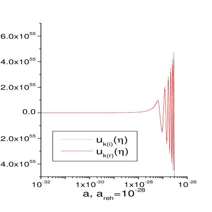
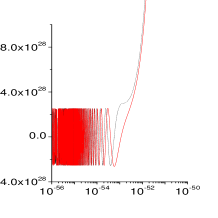
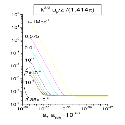
For a given $k$, we give our numerical results of the mode function $u_{k}$ in FIG. 1. From the figure we see that the mode function oscillates not only at the beginning of inflation, but also at the end of it. It oscillates at the end of inflation because $u_{k}(\eta)\propto\frac{a\dot{\phi}}{H}$ while $\dot{\phi}$ has oscillation behaviors during this time. However the quantity $\frac{k^{3/2}}{2\pi^{2}}|\frac{u_{k}(\eta)}{z}|$ keeps stable after the first period decreasing during inflation, see FIG. 1 and 2. We do not know whether the oscillation behavior of $u_{k}(\eta)$ at the end of inflation will have any observation implications, we note it here only because it was ignored by peoples for long time in researches.

Figure 1: Horizon axis, scale factor. Vertical axis, mode function $u_{k(i,r)}$, imaginary and real part. $k=0.3Mpc^{-1}$. $u_{k}$ oscillates not only at the beginning of inflation but also at the end of it. The inflation driving potential is $V(\phi)=m^{2}\phi^{2}/2$.

In numeric calculations, we take the integration starting point as the conformal time zero point. Using the oscillating properties (time translation invariant, up to a phase Salopek ; Adams ) of $u_{k}$ at the beginning of inflation, the initial conditions can be written as

$$u_{k(ini)}(\eta)=\frac{1}{\sqrt{2k}}e^{-ik\eta}|_{\eta=0}$$

$$w_{k(ini)}(\eta)=\sqrt{\frac{k}{2}}e^{-ik\eta}|_{\eta=0}$$ (11)

To solve the horizon, flatness and other pre-inflation problems, we require the universe expand $N_{e}=65$ e-foldings during inflation. The initial values of the scalar field has been tuned so that 65 e-foldings of inflations can be obtained. Assuming the reheating temperature is about $10^{15}Gev$ and the universe expand adiabatically in the standard big bang process, then at the initial point of integration, the scale factor is

$$a_{ini}=[e^{N_{e}}\frac{T_{reh}}{T_{tod}}]^{-1}=10^{-56},$$ (12)

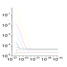
provided that the scale factor of today is set to $1$. However, if we let $k$ varies from $[10^{4}Mpc]^{-1}$ to $1Mpc^{-1}$ and integrate eqs(10) from $a=10^{-56}$ to $a=10^{-28}$ to get the full power spectrum, what we find will be a large scale suppressed result, see FIG. 2, 3 and the notes there.

The observational result of WMAP1 , if verified, favors a large scale suppressed power spectrum, but our suppressions here is due to an inconsistent initial conditions imposing. Because for very little $k$s, at the integration starting point $a_{ini}=10^{-56}$, $k^{-1}/(aH)^{-1}_{ini}\nrightarrow 0$. So eqs(11) cannot be taken as the correct initial conditions. For example, if we want to integrate eqs(1) in the simplest chaotic inflation model, $V(\phi)=m^{2}\phi^{2}/2$, $m=5.61\times 10^{-6}M_{pl}$ for $k=H_{0}=(4225Mpc)^{-1}$. To assure driving the universe expanding $10^{28}$ times during inflation, $\phi_{ini}=16.2M_{pl}$ BunnLiddleWhite . Then, at the integration starting point,

$$(aH)^{-1}_{ini} =[a_{ini}\sqrt{\frac{1}{3M^{2}_{pl}}V(\phi_{ini})}]^{-1}$$

$$=[10^{-56}\times 37.1\times 10^{-6}M_{pl}]^{-1}\sim 7082Mpc$$

Obviously, $k^{-1}/(aH)^{-1}_{ini}\sim 0.60\nrightarrow 0$, i.e. this $k$ mode of fluctuation is not well inside the horizon of that time. So, to use eqs(11) as the initial conditions, we have to integrate eqs(1) or equivalently eqs(10) beginning from a more little scale factor, say $a_{ini}=10^{-58}$ for example, so that those modes of fluctuations locate well inside the horizon of the integration starting point. Of course, the initial values of $\phi$ should be tuned correspondingly so that $10^{30}$ times of inflation can be obtained. Although works on the numerical calculations of the primordial power spectrum existed in several literatures Salopek ; Adams ; WenbingLin , none of them pointed out this problem explicitly, so we think it is worth noting here.

Figure 2: Horizon axis: scale factor, normalized by setting $a_{reh}=10^{-28}$. Vertical axis: quantity $\frac{k^{3/2}}{\sqrt{2}\pi}|\frac{u_{k}}{z}|$. Different curves corresponds to different $k$. Short vertical lines in the figure cross the curves at $aH=k$ point. Connecting centers of them yields the profile of the primordial power spectrum, see also the curves $c$ and $d$ of FIG. 3. Little figure: obtained by integrating eqs(10) from $a=10^{-56}$ to $a=10^{-28}$, taking eqs(11) as the initial conditions. Large figure: the same as the little one, but the scale factor varies from $10^{-58}$ to $10^{-28}$ and the initial values of $\phi$ is tuned correspondingly so that $10^{30}$ times of inflation can be obtained. The driving potential is $V(\phi)=m^{2}\phi^{2}/2$.

If we only let the universe expand $10^{26}\approx e^{60}$ BunnLiddleWhite times during inflation, the problem discussed above would be more serious.

III The Upper Bound on the Number of E-foldings of Inflation

However, if the number of e-foldings of inflation has an upper bound $N_{u.b.}$, then the comoving horizon of the universe will have an upper bound also. So as we trace back beyond this upper bound, the comoving horizon will decrease. Perturbations at scales larger than this upper bound will keep out of the horizon regardless how early we trace back to the origin of the universe. For such perturbations, the initial conditions eq(2) cannot be implemented physically.

Then, what is the upper bound? Is it large enough so that, at least for perturbations at scales of today’s Hubble horizon, the initial conditions eqs(2) can be implemented numerically? In string theories, by T. Banks and W. Fischler’s argument Banks1 , if the present acceleration of the universe is due to an asymptotically de Sitter universe with small cosmological constant, and the principle of Cosmological Complementary is valid, then the number of e-foldings of inflation is bounded. They estimated that $N_{u.b.}=65$. So the value already equals our assumed number of e-foldings of inflation required to solve the flatness, horizon and other pre-inflation problems in eqs(LABEL:horizon_criteria). Hence, if T. Banks and W. Fischler’s estimation is the case, then at least for perturbations at scales of today’s Hubble horizon, it will be impossible to implement the initial conditions (2) physically. Hence the power spectrum of such perturbations could not be nearly scale free any more. It could be suppressed strongly comparing with that of the little scale perturbations.

The second question is, if the number of e-foldings of inflation, consequently, the comoving horizon as we trace back to the origin of the universe has an upper bound, then, do perturbations at scales larger than this bound contribute to our observed CMBA? Recalling WMAP2 that, in calculating the multi-poles of CMBA, we need to do the following integration:

$$C_{l}=\int_{0}^{\infty}\frac{dk}{k}P_{\mathcal{R}}(k)[g_{l}^{\mathcal{R}}(k)]$$ (14)

where $P_{\mathcal{R}}(k)$ is the primordial power spectrum of perturbations produced during inflation and $g_{l}^{\mathcal{R}}(k)$ is the radiation transfer function. Mathematically, the integration should be made from $0$ to $\infty$. But physically, if some mechanism exists so that perturbations at scales greater than a certain cutoff wavelength $k_{c}^{-1}$ do not contribute to CMBA, then the lower bound of the integration (14) will be changed unavoidably.

Figure 3: Primordial power spectrum of density perturbations in Linde’s $\phi^{2}$ model. c: no suppression at all. d: large scale power suppressed by the inconsistent initial conditions.
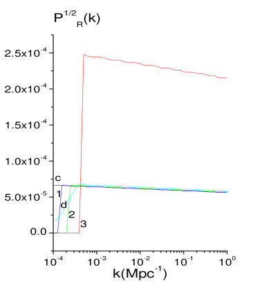
1: by assuming that $P_{\mathcal{R}}(k)=0$ for all $k<[7082Mpc]^{-1}$.
2: by assuming that $P_{\mathcal{R}}(k)=0$ for all $k<[4225Mpc]^{-1}$.
3: by assuming that $P_{\mathcal{R}}(k)=0$ for all $k<[2113Mpc]^{-1}$.

Figure 4: Theoretical curves is computed by CMBfast. Except the primordial power spectrum, see FIG. 3 and the notes there, other cosmic parameters are from WMAP’s best fitting $\Lambda CDM$ model. Scattered points are the observational results of WMAP2003 WMAP1 .

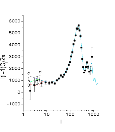
Obviously, if the number of e-foldings of inflation has an upper bound, then at the beginning of inflation, comoving horizon of the universe will reach its upper bound $[a_{i.b.}H_{i.b.}]^{-1}$ as we trace back to the origin of the universe. Perturbations beyond such a bound will keep out of the horizon regardless how early we trace back. We propose that such perturbations do not contribute to our observed CMBA. Our motivation is: from the beginning of inflation, these perturbations lie outside the horizon. They have no chances to experience a transition from quantum ones to classical ones before CMBA formed.

Under this assumption, we write the primordial power spectrum of perturbations produced during inflation as

$$P_{\mathcal{R}}(k) =0,\ k<k_{c}$$ (15)

$$=A\frac{k^{3}}{2\pi^{2}}|\frac{u_{k}}{z}|^{2}_{aH=k},\ k\geq k_{c}$$

where $A$ is a constant whose value can be determined by requiring that the corresponding primordial power spectrum gives approximately the same first peak CMBA multi-poles as observations, see FIG. 3 and 4, while $k_{c}$ is determined by the following relation:

$$k_{c}^{-1}=[a_{i.b.}H_{i.b.}]^{-1}$$ (16)

where the subscript $i.b.$ means that the relevant quantity take value when inflation begins.

$$a_{i.b.} =[e^{N_{u.b.}}\frac{T_{reh}}{T_{tod}}]^{-1}$$

$$H^{2}_{i.b.} \approx\frac{\Lambda_{infl}}{3M_{pl}^{2}}$$

$$k_{c}^{-1} \approx e^{N_{u.b.}}\frac{T_{reh}}{T_{tod}}\frac{\sqrt{3}M_{pl}}{\sqrt{\Lambda_{infl}}}$$ (17)

In the above equations, the scale factor of today is set to one, $N_{u.b.}$ denotes the upper bound on the number of e-foldings of inflation, $T_{reh}$ and $T_{tod}$ are the temperature of the universe at the reheating point and today respectively, while $\Lambda_{infl}$ is the characteristic energy scale of a given inflation model. We supposed that the universe enter the standard adiabatic expansion immediately after inflation.

Take T. Banks and W. Fischler’s estimation as an input and eqs(LABEL:horizon_criteria) as a guide post, where by the logic of eqs(17) $N_{u.b.}=65$, $T_{reh}\approx 10^{15}Gev$, $T_{tod}\approx 10^{-4}ev$, $\Lambda_{infl}=[m^{2}\phi^{2}/2]^{1/4}=8.01\times 10^{-3}M_{pl}$, we numerically calculated the CMBA multi-poles for three values of $k_{c}$

$$k_{c1,2,3}=[7082Mpc]^{-1},[4225Mpc]^{-1},[2113Mpc]^{-1}$$ (18)

where $7082Mpc$ could be considered as the largest sub-horizon perturbation scale under the assumption that $N_{u.b.}=65$; $4225Mpc$ is the perturbation scale corresponding to our today’s hubble horizon; while $2113Mpc$, half of that. Our results are displayed in FIG. 3 and 4, curves 1, 2, 3. From the figure we see that the little $l$ multi-poles of CMBA is very sensitive to the cutoff of the primordial power spectrum. If $k_{c}$ takes a certain value between $k_{c2}$ and $k_{c3}$, then theoretical curves will tally with the observational results to a better degree.

So, if the number of e-foldings of inflation has an upper bound, and by our proposition, perturbations outside the horizon at the inflation beginning point do not affect the large scale structure formation at late times, then the exceptional lowness of the little $l$ multi-poles of CMBA can be reproduced numerically. In Linde’s $\phi^{2}$ inflation model, which has characteristic energy $\Lambda\approx 10^{-2}M_{pl}$, the upper bound on the number of e-foldings of inflation is approximately $65$. In other inflation models, if the observational result are to be reproduced, by eq(17), more lower characteristic inflation energy will mean a more little upper bound on the number of e-foldings, and vice versa.

When this paper is posted in the network, we are noted that in reference Stochastic , the authors studied the stochastic inflation mechanism and got similar results like ours. In some sense, the mechanisms there can be assimilated to another statement of a limited number of e-foldings of inflation.

IV Summary

In this paper, we first present four notes on calculations of the primordial power spectrum of perturbations produced during inflation. 1st, to get the nearly scale free power spectrum of perturbation, it is unnecessary to use the asymptotic behavior of the Hankel function as its argument goes to 0. 2nd, scale factor $a$ is a better independent variable than $lna$ in the numerical integrations of the Friedmann-Mukhanov equations. 3rd, the perturbation mode function $u_{k}$ oscillates both at the initial and the end of inflation times. 4th, numerically, to implement the initial conditions of the perturbation equations consistently, we must let the universe experience more number of e-foldings inflation than that required of it to solve the horizon, flatness and other pre-inflation problems.

We then explore effects from the existence of an upper bound on the number of e-foldings of inflation on the implementation of the initial conditions required of the perturbation mode function. When such an upper bound exists, the comoving horizon of the universe will have an upper bound also as we trace back to the origin of the universe. So perturbations at scales beyond this bound will keep outside the horizon regardless how early we trace back in the history of the universe. After proposing that such perturbations do not affect the formation of CMBA, we find the observed exceptional lowness of the little $l$ multi-poles of CMBA could be reproduced numerically. In Linde’s $\phi^{2}$ model, the upper bound on the number of e-foldings of inflation is determined to be 65 approximately.

Acknowledgments: We would like to thank professor M. Li for discussions.

References

- (1) C. L. Bennett etc, Astrophys. J. Suppl. 148: 1, 2003.
- (2) L. Verde etc, Astrophys. J. Suppl. 148: 195, 2003.
- (3) E. D. Stewart and D. H. Lyth, Phys. Lett. B302: 171-175, 1993.
- (4) V. F. Mukhanov, H. A. Feldman and R. H. Brandenberger, Phys. Rep. 215(1992)203.
- (5) E. F. Bunn, A. R. Liddle and M. White, Phys. Rev. D54: R5917, 1996.
- (6) D. S. Salopek, J. R. Bond and J.M.Bardeen, Phys. Rev. D40: 1753, 1989.
- (7) J. Adams, B. Cresswell and R. Easther, Phys. Rev. D64: 123514, 2001.
- (8) D. H. Huang, W. B. Lin, X.M. Zhang, Phys. Rev. D62: 087302, 2000.
- (9) W. H. Press, S. A. Teukolsky etc, Numerical Recipes in C, Secod Edition(Cambrige University Press, Cambrige, 1992).
- (10) T. Banks and W. Fischler (2004) [astro-ph/0307459] By M. Liguori,
-
(11)
S. Matarrese, M. Musso and A.Riotto, JCAP 0405: 008, 2004
M.Liguori, S.Matarrese, M.Musso and A.Riotto, JCAP 0408: 011, 2004.