Constraining Dark Energy with X-ray Galaxy Clusters, Supernovae and the Cosmic Microwave Background

Abstract

We present new constraints on the evolution of dark energy from an analysis of Cosmic Microwave Background, supernova and X-ray galaxy cluster data. Our analysis employs a minimum of priors and exploits the complementary nature of these data sets. We examine a series of dark energy models with up to three free parameters: the current dark energy equation of state $w_{\rm 0}$, the early time equation of state $w_{\rm et}$ and the scale factor at transition, $a_{\rm t}$. From a combined analysis of all three data sets, assuming a constant equation of state and that the Universe is flat, we measure $w_{\rm 0}=-1.05^{+0.10}_{-0.12}$. Including $w_{\rm et}$ as a free parameter and allowing the transition scale factor to vary over the range $0.5<a_{\rm t}<0.95$ where the data sets have discriminating power, we measure $w_{\rm 0}=-1.27^{+0.33}_{-0.39}$ and $w_{\rm et}=-0.66^{+0.44}_{-0.62}$. We find no significant evidence for evolution in the dark energy equation of state parameter with redshift. Marginal hints of evolution in the supernovae data become less significant when the cluster constraints are also included in the analysis. The complementary nature of the data sets leads to a tight constraint on the mean matter density, $\Omega_{\rm m}$ and alleviates a number of other parameter degeneracies, including that between the scalar spectral index $n_{\rm s}$, the physical baryon density $\Omega_{\rm b}h^{2}$ and the optical depth $\tau$. This complementary nature also allows us to examine models in which we drop the prior on the curvature. For non-flat models with a constant equation of state, we measure $w_{\rm 0}=-1.09^{+0.12}_{-0.15}$ and obtain a tight constraint on the current dark energy density, $\Omega_{\rm de}=0.70\pm 0.03$. For dark energy models other than a cosmological constant, energy–momentum conservation requires the inclusion of spatial perturbations in the dark energy component. Our analysis includes such perturbations, assuming a sound speed $c_{\rm s}^{2}=1$ in the dark energy fluid as expected for Quintessence scenarios. For our most general dark energy model, not including such perturbations would lead to spurious constraints on $w_{\rm et}$ which would be tighter than those mentioned above by approximately a factor two with the current data.

1 Introduction

The precise measurement of the Cosmic Microwave Background (CMB) made with the Wilkinson Microwave Anisotropy Probe (WMAP) (Hinshaw et al., 2003; Kogut et al., 2003) has improved our knowledge of a wide range of cosmological parameters. However, a number of degeneracies between parameters exist which cannot be broken with current CMB data alone and which require the introduction of other, complementary data sets.

Some of the most important parameters and degeneracies concern dark energy and its equation of state. Since observations of distant type Ia supernovae (SNIa) first indicated that the expansion of the Universe is accelerating (Riess et al., 1998; Perlmutter et al., 1999), there has been enormous interest in this topic. The most straightforward way to incorporate an accelerated expansion into cosmological models is by adding a constant term to the Einstein equations - the cosmological constant. However, this leads to an extreme fine tuning problem wherein one must adjust the initial density of this constant to $10^{-120}M_{\rm pl}^{4}$ in natural Planck units. To alleviate this, a scalar field model, dubbed Quintessence, was introduced which, when the potential is carefully chosen, can avoid the fine tuning of initial conditions (Peebles & Ratra, 1988; Ratra & Peebles, 1988; Wetterich, 1988; Ferreira & Joyce, 1998; Caldwell et al., 1998; Zlatev et al., 1999). When describing the background evolution of the Universe with such models, it is sufficient to know the equation of state for the dark energy i.e. the ratio of pressure and energy density, $w=p_{\rm de}/\rho_{\rm de}$. Whilst a cosmological constant has $w=-1$ at all times, for most dark energy models the equation of state parameter is an evolving function of redshift, $w=w(z)$.

In order to learn more about the origin of cosmic acceleration and dark energy, it is crucial to constrain the evolution of the dark energy equation of state. In the first case, this requires us to examine whether the accelerated expansion can be described by a cosmological constant or if there is need to go beyond this description. Most early attempts to parameterise the evolution of dark energy were carried out as feasibility studies for future supernovae experiments (Huterer & Turner, 1999; Efstathiou, 1999; Saini et al., 2000; Maor et al., 2001; Astier, 2001; Weller & Albrecht, 2001, 2002). However, recent improvements in the data for high-redshift SNIa and the arrival of other, complementary constraints means that we can now start to ask the same questions of real data (Knop et al., 2003; Riess et al., 2004).

The data for SNIa can be used to measure the luminosity distances to these sources independent of their redshifts. This constrains a combination of the dark matter and dark energy densities in a different way to observations of CMB anisotropies. The combination of the two data sets is therefore useful in breaking parameter degeneracies. However, the simplest, linear expansion in redshift for the dark energy equation of state advocated by e.g. Maor et al. (2001), Astier (2001) and Weller & Albrecht (2001, 2002) cannot be applied to the high redshifts probed by the CMB. For this reason, the linear parameterisation was extended by Chevallier & Polarski (2001) and Linder (2003) to a model in which the equation of state at low redshifts (late times) $w_{\rm 0}$, and at high redshifts (early times) $w_{\rm et}$, could be specified separately. Although more suitable than the low redshift linear expansion for the analysis of CMB data, this parameterisation also has a short-coming in that the transition between $w_{\rm 0}$ and $w_{\rm et}$ always occurs at redshift $z=1$ and with a fixed transition rate, which is not representative of the full range of scalar field dark energy models of interest (see e. g. Weller & Albrecht (2002)). Corasaniti et al. (2003) and Bassett et al. (2004) extended this prescription further, allowing the transition to occur at an arbitrary time and rate. Corasaniti et al. (2004) applied this extended model to a combination of SNIa, CMB and galaxy redshift survey data, noting the presence of strong degeneracies between a number of the derived parameters. The analysis of Corasaniti et al. (2004) included a limited exploration of models with an equation of state $w<-1$: so called phantom models (Caldwell, 2002). While the extension to $w<-1$ is challenging in terms of the physics involved (Carroll et al., 2003), it is interesting from a phenomenological point of view, particularly given that the best-fit to current supernovae data is obtained for models with $w<-1$ (Riess et al., 2004).

It is important to note that the analysis of Corasaniti et al. (2004) did not include dark energy perturbations for models crossing $w=-1$. While a cosmological constant is spatially homogeneous, this is not true for an arbitrary dark energy fluid or Quintessence. One must include perturbations in the dark energy component, not just for consistency reasons but also because the exclusion of them can lead to erroneously tight constraints on $w$ from large-scale CMB anisotropies (Weller & Lewis, 2003).

It was realised by Maor et al. (2001) and Weller & Albrecht (2001, 2002) that in order to constrain the evolution of the equation of state with supernovae observations, it is necessary to use a tight prior on the mean matter density of the Universe, $\Omega_{\rm m}$. Recent measurements of the gas fraction in X-ray luminous, dynamically relaxed clusters made with the Chandra X-ray Observatory provide one of our best constraints on $\Omega_{\rm m}$ (Allen et al., 2004). These data also provide a direct and independent method by which to measure the acceleration of the Universe, providing additional discriminating power for dark energy studies. As we shall demonstrate here, the combination of CMB and X-ray cluster data can also play an important role in breaking other key parameter degeneracies (see also Allen et al. (2003)). For these reasons, we have used a combination of X-ray gas fraction, CMB and SNIa data in this study.

In the following sections we first introduce our choice of parameterisations for the dark energy equation of state. We then discuss the individual data sets and how they probe cosmology. Our results are presented in Section 4. Section 5 discusses the results and summarises our conclusions.

2 Dark Energy Model

A number of different parameterisations for the evolution of the dark energy equation of state parameter, $w(z)$, have been discussed in the literature. The simplest is the linear parameterisation: $w(z)=w_{\rm 0}+w^{\prime}z$ (Maor et al., 2001; Weller & Albrecht, 2001, 2002; Astier, 2001). However, as mentioned above, this model is not compatible with CMB data since it diverges at high redshift. Chevallier & Polarski (2001) (see also Linder (2003)) proposed an extended parameterisation which avoids this problem, with $w(z)=w_{\rm 0}+w_{1}z/(1+z)$. This model can in principle be used to distinguish a cosmological constant from other forms of dark energy with a varying $w$. However, this parameterisation is not representative of standard Quintessence models. Corasaniti et al. (2003) proposed a generalised parameterisation which is better suited to the problem. However, that model includes four parameters and exhibits large degeneracies when applied current data.

Here, we use an extension of the model discussed by Chevallier & Polarski (2001) and Linder (2003), which stops short of the full extension suggested by Corasaniti et al. (2003). The primary short-coming of the parameterisation proposed by Chevallier & Polarski (2001); Linder (2003) is that it uses a fixed redshift, $z=1$, for the transition between the current value of the equation of state and the value at early times, $w_{\rm et}=w_{\rm 0}+w_{1}$. Our model introduces one extra parameter, $z_{\rm t}$, the transition redshift between $w_{\rm et}$ and $w_{\rm 0}$, such that

$$w=\frac{w_{\rm et}z+w_{\rm 0}z_{\rm t}}{z+z_{\rm t}}=\frac{w_{\rm et}(1-a)a_{\rm t}+w_{\rm 0}(1-a_{\rm t})a}{a(1-2a_{\rm t})+a_{\rm t}}\;,$$ (1)

where $a_{\rm t}$ is the transition scale factor. (The parameterisation of Corasaniti et al. (2003) also introduces an arbitrary transition rate between $w_{\rm 0}$ and $w_{\rm et}$.)

Energy conservation of the dark energy fluid results in evolution of the energy density with the scale factor, such that

$$\rho_{\rm de}(a)=\rho_{{\rm de,}0}a^{-3}e^{-3\int_{1}^{a}{\frac{w(a^{\prime})}{a^{\prime}}da^{\prime}}},\;$$ (2)

where $\rho_{{\rm de,}0}$ is the energy density of the dark energy fluid today. Using the parameterisation of equation (1) we obtain

$$\int_{1}^{a}{\frac{w(a^{\prime})}{a^{\prime}}da^{\prime}}=w_{\rm et}\ln a+(w_{\rm et}-w_{\rm 0})g(a;a_{\rm t})\;,$$ (3)

with

$$g(a;a_{\rm t})=\left(\frac{1-a_{\rm t}}{1-2a_{\rm t}}\right)\ln\left(\frac{a(1-a_{\rm t})}{a(1-2a_{\rm t})+a_{\rm t}}\right)\;.$$ (4)

Setting $z_{\rm t}=1$ or $a_{\rm t}=1/2$, we recover the parameterisation of Linder (2003). Hereafter, we shall refer to this as the $z_{\rm t}=1$ dark energy model. From the Friedmann equation, the evolution of the Hubble parameter $H(z)=H_{0}E(z)$ is given by

$$E(z)=\sqrt{\Omega_{\rm m}(1+z)^{3}+\Omega_{\rm de}f(z)+\Omega_{\rm k}(1+z)^{2}}\;,$$ (5)

with

$$f(z)=(1+z)^{3(1+w_{\rm et})}e^{-3(w_{\rm et}-w_{\rm 0})g(z;z_{\rm t})},$$ (6)

where $\Omega_{\rm m}$, $\Omega_{\rm de}$, $\Omega_{\rm k}$ are the matter, dark energy and curvature densities in units of the critical density.

3 Data Analysis

We have performed a likelihood analysis using three cosmological data sets: CMB, SNIa and the X-ray cluster gas fraction.

For the CMB analysis we have modified the camb code (Lewis et al., 2000) to include the relevant dark energy equation of state parameters. For the calculation of CMB spectra, we have accounted for the effects perturbations in the dark energy component (Weller & Lewis, 2003). We assume that the sound speed of the dark energy fluid, $c_{\rm s}^{2}=1$, a choice that is well motivated for standard Quintessence scenarios (Weller & Lewis, 2003), although some other well-motivated dark energy models such as k–essence scenarios (Armendariz–Picon et al., 2000) include an evolving sound speed. We note the presence of an extra term in the perturbation equations due to the variation of the equation of state with time, which sources the density perturbation with the velocity perturbation. This effect will be discussed in a forthcoming publication (Rapetti & Weller, 2005).

We use three CMB data sets: WMAP (Verde et al., 2003; Hinshaw et al., 2003; Kogut et al., 2003) (including the temperature-polarization cross-correlation data), the Cosmic Background Imager (CBI) (Pearson et al., 2003) and the Arcminute Cosmology Bolometer Array Receiver (ACBAR) (Kuo et al., 2004). The latter data sets provide important information on smaller scales ($\ell>800$).

For the SNIa analysis, we use the gold sample of Riess et al. (2004), marginalising analytically over the absolute magnitude $M$ as a “nuisance parameter”. We fit the extinction-corrected distance moduli, $\mu_{0}=m-M=5\log d_{L}+25$, where $m$ is the apparent magnitude and $d_{L}$ is the luminosity distance in units of Mpc defined as

$$d_{L}=\frac{c(1+z)}{H_{0}\sqrt{\Omega_{k}}}{\rm sinh}\left(\sqrt{\Omega_{k}}\int_{0}^{z}\frac{dz}{\sqrt{E(z)}}\right)\;,$$ (7)

where $\Omega_{\rm k}=1-\Omega_{\rm m}-\Omega_{\rm de}$.

Figure 1: The 68.3 and 95.4 per cent confidence limits in the $(\Omega_{\rm m},w_{\rm 0})$ plane for the various pairs of data sets and for all three data sets combined. A constant dark energy equation of state parameter is assumed.

For the X-ray gas mass fraction analysis, we use the data and method of Allen et al. (2004), fitting the apparent redshift evolution of the cluster gas fraction with the model

$$f_{\rm gas}^{\rm SCDM}(z)=\frac{b\,\Omega_{\rm b}}{\left(1+0.19\sqrt{h}\right)\Omega_{\rm m}}\left[\frac{d_{\rm A}^{\rm SCDM}(z)}{d_{\rm A}^{\rm de}(z)}\right]^{1.5}\;,$$ (8)

where $d_{\rm A}^{\rm de}(z)$ and $d_{\rm A}^{\rm SCDM}(z)$ are the angular diameter distances ($d_{A}=d_{L}/(1+z)^{2}$) to the clusters for a given dark energy (de) model and the reference standard cold dark matter cosmology, respectively. $\Omega_{\rm b}$ is the mean baryonic matter density of the Universe in units of the critical density, $H_{0}=100\,h\,{\rm km}\,{\rm sec}^{-1}\,{\rm Mpc}^{-1}$ and $b$ is a bias factor that accounts for the (relatively small amount of) baryonic material expelled from galaxy clusters as they form. Following Allen et al. (2004), we adopt a Gaussian prior on $b=0.824\pm 0.089$, which is appropriate for clusters of the masses studied here. Note that the prior on $b$ includes a 10 per cent allowance for systematic uncertainties in the normalisation of the $f_{\rm gas}(z)$ curve, although we note that even doubling this systematic uncertainty has only a small effect on the results (Allen et al., 2004).

Figure 2: (Left panel) The marginalised constraints on $w_{\rm 0}$ assuming a constant dark energy equation of state. The solid line is for all the three data sets together, the short dashed line for clusters+CMB, the long-dashed line for SNIa+CMB, and the dot-dashed line for clusters+SNIa (with priors from HST and BBN). The right panel shows the marginalised constraints on $\Omega_{\rm m}$ for each combination of data sets.

We have included our extension of the camb code into the cosmomc package, which provides an efficient sampling of the posterior likelihoods using a Markov Chain Monte Carlo (MCMC) algorithm  (Lewis & Bridle, 2002). We have also included the Riess et al. (2004) supernovae sample and the Allen et al. (2004) gas fraction data into the analysis, using the cosmomc code to calculate the posterior probability densities.

For our standard analysis we have varied nine “cosmological” parameters: the baryon density $\Omega_{\rm b}h^{2}$, the cold dark matter density $\Omega_{\rm dm}h^{2}$, the Hubble constant $H_{\rm 0}$, the reionisation redshift $z_{\rm re}$, the spectral index $n_{\rm s}$, the amplitude of the fluctuations $A_{\rm s}$ and the dark energy equation of state parameters $w_{\rm 0}$, $w_{\rm et}$ and $a_{\rm t}$. We assume zero tensor components and a negligible neutrino mass. The bias parameter $b$ associated with the X-ray cluster data is an additional parameter in the fits. We have marginalised analytically over the intrinsic magnitude $M$ of the supernovae. Except where stated otherwise, our analysis assumes that the Universe is flat ($\Omega_{\rm k}=0$). For the analysis of the cluster data without the CMB data, we use Gaussian priors on $\Omega_{\rm b}h^{2}=0.0214\pm 0.0020$ from Big Bang Nucleosynthesis (BBN) constraints (Kirkman et al., 2003) and $h=0.72\pm 0.08$ from observations made with the Hubble Space Telescope (HST) (Freedman et al., 2001).

Table 1: The median values and 68.3 per cent confidence intervals from the analysis of the various pairs of data sets and for all three data sets combined, assuming a constant dark energy equation of state. The last column states the $\chi^{2}$ per degree of freedom for each combination of data sets.

Data combination	$w_{\rm 0}$	$\Omega_{\rm m}$	$\chi^{2}/dof$
Cl+CMB	$-1.23^{+0.17}_{-0.21}$	$0.254^{+0.037}_{-0.034}$	1467.4/1378
Cl+SN(+HST+BBN)	$-1.04^{+0.14}_{-0.18}$	$0.288^{+0.043}_{-0.040}$	210.2/178
SN+CMB	$-1.04^{+0.13}_{-0.16}$	$0.312^{+0.041}_{-0.044}$	1625.9/1508
Cl+SN+CMB	$-1.05^{+0.10}_{-0.12}$	$0.295^{+0.031}_{-0.027}$	1652.5/1534

Figure 3: The 68.3 and 95.4 per cent confidence limits in the $(\Omega_{\rm m},w_{\rm 0})$ plane for the various pairs of data sets and for all three data sets combined. The $z_{\rm t}=1$ dark energy model is assumed.

For each different model+data combination, we have sampled four independent MCMC chains. The length of these chains vary from the simplest models of constant equation of state with around six thousand samples per chain up to our most general model with around one hundred and fifty thousand samples per chain. We have applied the Gelman-Rubin criterion to test for convergence (Gelman & Rubin, 1992). Convergence is assumed to be acceptable if the ratio of the between-chain and mean-chain variances satisfies $R-1<0.1$. We have also checked for convergence by ensuring that consistent final results are obtained from sampling numerous small subsets of the chains.

Figure 4: The 68.3 and 95.4 per cent confidence limits in the ($\Omega_{\rm m}$;$w_{\rm 0}$,$w_{\rm et}$) plane for all three data sets combined using various fixed values for the transition redshift. The solid lines show the results on ($\Omega_{\rm m}$,$w_{\rm 0}$). The dashed lines show the results on ($\Omega_{\rm m}$,$w_{\rm et}$). The left panel is for $z_{\rm t}=1$ ($a_{\rm t}=0.5$), the centre panel $z_{\rm t}=0.11$ ($a_{\rm t}=0.9$) and the right panel $z_{\rm t}=0.35$ ($a_{\rm t}=0.74$). The uncertainty in $w_{\rm et}$ is much larger than for $w_{0}$ in the left panel, which reflects the paucity of data at high redshifts. The $z_{\rm t}=0.35$ transition splits the cluster and SNIa data into similarly sized low and high redshift subsamples. The horizontal dotted line denotes the cosmological constant model ($w_{\rm 0}=w_{\rm et}=-1$).

4 Dark Energy constraints

We have employed a series of different parameterisations for the dark energy equation of state: (i) $w$ constant (ii) a model with $w_{\rm 0}$ and $w_{\rm et}$ free, but with the transition redshift fixed at $z_{\rm t}=1$ ($a_{\rm t}=0.5$) (iii) a similar model with the transition fixed at $z_{\rm t}=0.11$ ($a_{\rm t}=0.9$) (iv) a similar model with the transition fixed at $z_{\rm t}=0.35$ ($a_{\rm t}=0.74$), which approximately splits the cluster and supernovae data about their median redshifts and (v) a model in which the transition redshift is a free parameter.

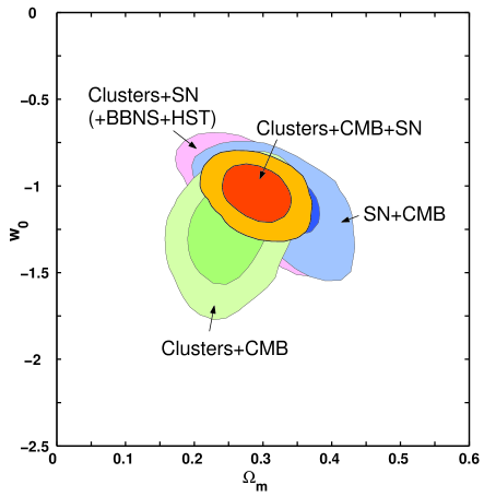
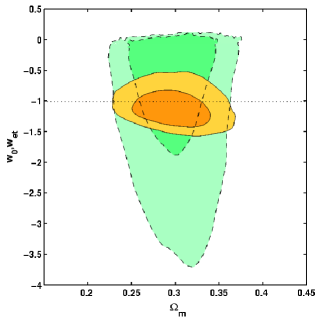
Figure 1 shows the constraints on $w_{\rm 0}$ and $\Omega_{\rm m}$ for the constant dark energy equation of state model. We see that the combination of the three data sets leads to tight constraints on $w_{\rm 0}$ and $\Omega_{\rm m}$, which are in good agreement with the cosmological constant scenario ($w_{\rm 0}=-1$). This figure also demonstrates the complementary nature of the constraints provided by the various pairs of data sets, in particular SNIa+CMB and clusters+CMB.

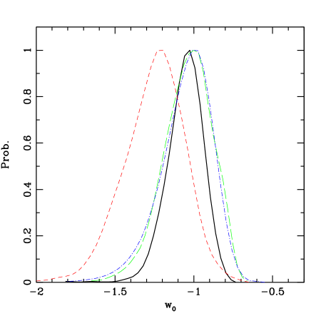
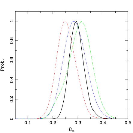
The power of the combined clusters+SNIa+CMB data set is also evident in the marginalised probability distributions for $w_{\rm 0}$ (left panel of Figure 2) and $\Omega_{\rm m}$ (right panel). The marginalised 68.3 per cent confidence limits on $w_{\rm 0}$ and $\Omega_{\rm m}$ for the various data combinations, assuming a constant dark energy equation of state, are summarised in Table 1.

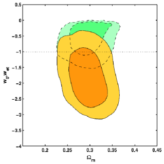
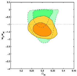
Figure 3 shows the results obtained using the $z_{\rm t}=1$ dark energy model. Comparison of Figs 1 and 3 shows how the joint confidence contours on ($\Omega_{\rm m}$,$w_{\rm 0}$) open up when $w_{\rm et}$ is introduced as an additional free parameter. This is particularly prominent for the clusters+CMB combination where the $w_{\rm 0}$ region is extended into the positive branch due to the degeneracy between $w_{\rm 0}$ and $w_{\rm et}$, discussed below. The results on $w_{\rm 0}$ and $w_{\rm et}$ for the $z_{\rm t}=1$ model are shown in the left panel of Figure 4. The figure shows how, for this model, the present data constrain $w_{\rm 0}$ more tightly than $w_{\rm et}$. This simply reflects the paucity of cluster and SNIa data at redshifts beyond $z_{\rm t}=1$. Note that the CMB data provide an upper limit of $w_{\rm et}\lesssim 0$ at high redshifts; for $w_{\rm et}>0$, the dark energy component would become significant at early times, causing modifications to the predicted CMB anisotropy spectrum.

Figure 5: The 68.3 and 95.4 per cent confidence limits in the ($w_{\rm 0}$,$w_{\rm et}$) plane obtained using the SNIa+CMB (blue, thin solid), Clusters+CMB (green, long–dashed) and Clusters+SNIa(+BBN+HST) (magenta, dotted) data sets. The bold lines show the results for all three data sets combined and the dark circle marks the cosmological constant model. The dashed line shows the no evolution models ($w_{\rm 0}=w_{\rm et}$). The transition redshift is fixed to $z_{\rm t}=0.35$ in all cases.

Table 2: The median parameter values and values at the peaks of the marginalised probability distributions (and 68.3 per cent confidence intervals) for the various dark energy parameterisations, using all three data sets combined. Results are listed for both flat and non-flat priors. The last column states the $\chi^{2}$ per degree of freedom for each parameterisation.

equation of state	median $w_{\rm 0}$	median $w_{\rm et}$	median $\Omega_{\rm m}$	Peak $w_{\rm 0}$	Peak $w_{\rm et}$	Peak $\Omega_{\rm m}$	$\chi^{2}/dof$
constant (flat)	$-1.05^{+0.10}_{-0.12}$	-	$0.295^{+0.031}_{-0.027}$	$-1.04\pm 0.10$	-	$0.293\pm 0.028$	1652.5/1534
constant (non flat)	$-1.09^{+0.12}_{-0.15}$	-	$0.314^{+0.040}_{-0.036}$	$-1.02^{+0.08}_{-0.20}$	-	$0.31^{+0.04}_{-0.05}$	1651.3/1533
$z_{\rm t}=1$ (flat)	$-1.10^{+0.23}_{-0.19}$	$-0.87^{+0.61}_{-1.10}$	$0.300^{+0.029}_{-0.028}$	$-1.16^{+0.22}_{-0.19}$	$-0.05^{+0.09}_{-1.17}$	$0.30\pm 0.03$	1650.6/1533
$z_{\rm t}=1$ (non flat)	$-1.08^{+0.30}_{-0.23}$	$-1.23^{+0.86}_{-2.06}$	$0.328^{+0.046}_{-0.040}$	$-1.14^{+0.31}_{-0.21}$	$-0.09^{+0.12}_{-2.16}$	$0.32^{+0.04}_{-0.05}$	1648.1/1532
split, $z_{\rm t}=0.35$ (flat)	$-1.30^{+0.34}_{-0.28}$	$-0.61^{+0.40}_{-0.62}$	$0.300^{+0.028}_{-0.027}$	$-1.49^{+0.41}_{-0.20}$	$-0.10^{+0.09}_{-0.71}$	$0.30\pm 0.03$	1649.0/1533
arbitrary $z_{\rm t}$ (flat)	$-1.27^{+0.33}_{-0.39}$	$-0.66^{+0.43}_{-0.62}$	$0.299^{+0.029}_{-0.027}$	$-1.23^{+0.34}_{-0.46}$	$-0.12^{+0.11}_{-0.76}$	$0.298\pm 0.028$	1648.9/1532

It is important to recognise that the choice of transition redshift, $z_{\rm t}=1$, described above is arbitrary. We have therefore examined the constraints obtained for other values of $z_{\rm t}$ ($a_{\rm t}$). The centre panel of Figure 4 shows the results using a late transition model with $z_{\rm t}=0.11$ ($a_{\rm t}=0.9$). We see that the cosmological constant ($w_{\rm 0}=w_{\rm et}=-1$) again lies within the allowed 68.3 per cent confidence ($1\sigma$) regions. Unsurprisingly, the constraints on $w_{\rm et}$ in the late transition case are better than for the $z_{\rm t}=1$ model, reflecting the presence of more cluster and SNIa data beyond the transition redshift. Naturally, this at the expense of a weaker constraint on $w_{\rm 0}$.

If we select a transition redshift close to the median redshift for the SNIa and cluster data sets, one might expect to obtain comparable constraints on $w_{\rm 0}$ and $w_{\rm et}$. In principle, this approach could provide improved sensitivity when searching for evolution in the equation of state parameter. (In detail, we expect the constraints on $w_{\rm 0}$ to be slightly better than those for $w_{\rm et}$ using the median redshift model, since the precision of the individual cluster and supernova measurements are lower at high redshifts.) The right panel of Figure 4 shows the results obtained fixing $z_{\rm t}=0.35$ ($a_{\rm t}=0.74$), a redshift close to the median redshift for both the cluster and SNIa data sets. In this case the uncertainties on $w_{\rm 0}$ and $w_{\rm et}$ are indeed similar and the combined size of the confidence regions is reduced. However, the cosmological constant remains an acceptable description of the data. The marginalised results on $w_{\rm 0}$, $w_{\rm et}$ and $\Omega_{\rm m}$ are summarised in Table 2.

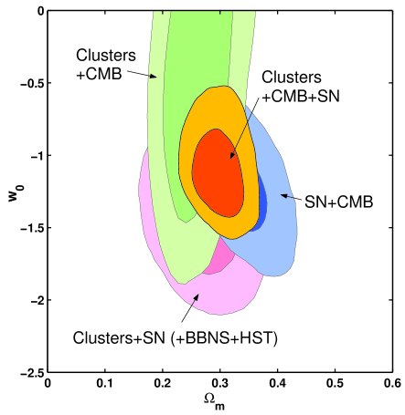
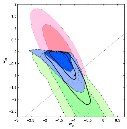
Within the context of searching for evolution in the dark energy equation of state, it is interesting to note the constraints that arise from the combinations of SNIa+CMB, clusters+CMB and clusters+SNIa(+BBN+HST) data separately. Figure 5 shows the results in the ($w_{\rm 0},w_{\rm et}$) plane for the three pairs of data sets and for all three data sets combined, using the $z_{\rm t}=0.35$ dark energy model. We see that the combination of SNIa+CMB data provides marginal evidence for evolution in the equation of state, in that the 68.3 per cent confidence contours exclude the no evolution line ($w_{\rm 0}=w_{\rm et}$). However, the clusters+CMB and clusters+SNIa data are consistent with the cosmological constant at the 68.3 per cent level, and the effect of combining all three data sets (bold contours in Figure 5) is to remove the marginal evidence for evolution hinted at in the SNIa+CMB data alone.

Figure 6: The distribution of MCMC samples in the ($w_{\rm 0}$,$w_{\rm et}$) plane for the case of a transition scale factor allowed to vary over the range $0<a_{\rm t}<1$. The colours indicate the value of $a_{\rm t}$.

Figure 7: (Left panel) The 68.3 and 95.4 per cent confidence limits in the ($\Omega_{\rm m}$;$w_{\rm 0}$,$w_{\rm et}$) plane for a general dark energy model with the transition scale factor allowed to vary over the range $0.5<a_{\rm t}<0.95$. The solid lines show the results on ($\Omega_{\rm m}$,$w_{\rm 0}$). The dashed lines show the results on ($\Omega_{\rm m}$,$w_{\rm et}$). The horizontal dotted line denotes the cosmological constant model ($w_{\rm 0}=w_{\rm et}=-1$). (Right panel) The constraints in the ($w_{\rm 0}$,$w_{\rm et}$) plane for the above model (bold, solid lines). For comparison, the constraints obtained for the various fixed transition redshifts are also shown: $z_{\rm t}=1.0$ (green, dashed), $z_{\rm t}=0.35$ (blue, thin solid), $z_{\rm t}=0.11$ (red, dotted). The dark circle marks the cosmological constant model.

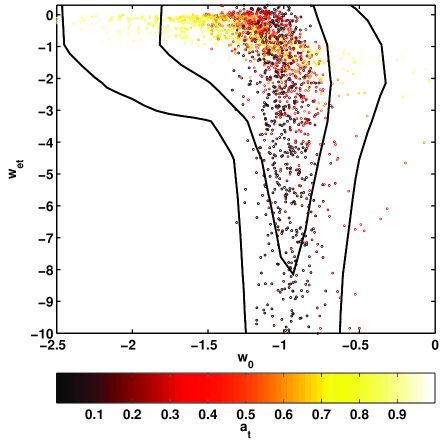
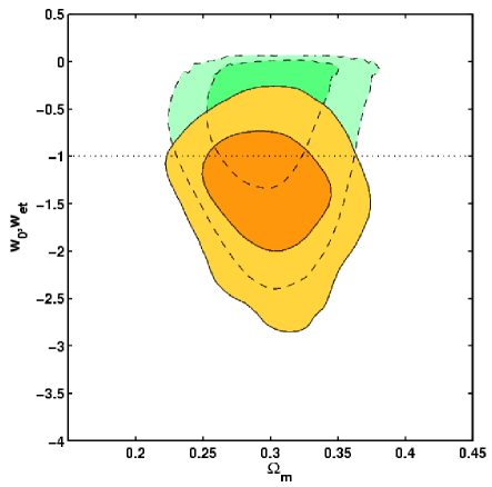
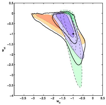
Figure 5 clearly shows the degeneracies between $w_{\rm 0}$ and $w_{\rm et}$ for the different data combinations, and demonstrates the importance of including the CMB data when attempting to obtain the best constraints on $w_{\rm 0}$ and $w_{\rm et}$. Comparing the dotted contours [clusters+SNIa+(BBN+HST)] with the bold contours [clusters+SNIa+CMB] one sees that as well as providing a tight upper limit on $w_{\rm et}$ as discussed above, the inclusion of the CMB data also leads to tighter constraints on $w_{\rm 0}$ and the exclusion of large negative values for $w_{\rm et}$.

The most general dark energy model we have examined includes $w_{\rm 0}$, $w_{\rm et}$ and the transition scale factor, $a_{\rm t}$, as free parameters. In the first case, $a_{\rm t}$ was allowed to take any value in the range $0<a_{\rm t}<1$. The distribution of MCMC samples from this analysis is shown in Figure 6. This figure re-emphasises the point that when the transition in the dark energy equation of state occurs at late times (low redshifts; light coloured sample points) $w_{\rm et}$ is confined to a relatively narrow band ($-2\lesssim w_{\rm et}\lesssim 0$) and the constraint on $w_{\rm 0}$ is poor ($-2.5\lesssim w_{\rm 0}\lesssim-0.5$). When the transition occurs earlier (at high redshifts; darker points), the constraint on $w_{\rm 0}$ is improved and the constraint on $w_{\rm et}$ is weakened. In this case, some sample points even populate the region beyond $w_{\rm et}>0$. [If the transition occurs at sufficiently early times, even the CMB data cannot provide a tight limit on $w_{\rm et}$. It is likely, however, that an early equation of state with $w\gtrsim 1/3$ violates BBN bounds, if the dark energy component is significant at the time when the BBN species freeze out (Bean et al., 2001).]

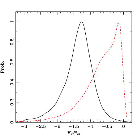
It is clear from Fig 6 that interesting constraints on both $w_{\rm 0}$ and $w_{\rm et}$ can only be obtained when the transition redshift is restricted to lie within the range spanned by the cluster and SNIa data. Otherwise large peaks in the marginalised probability distributions will occur that will simply reflect an inability to distinguish between models with transition redshifts beyond the range of the present data. For this reason, we have carried out a second analysis in which $a_{\rm t}$ was allowed to vary only over the range $0.5<a_{\rm t}<0.95$; a sensible compromise given the current cluster and SNIa data. Fig 7 shows the confidence contours in the ($\Omega_{\rm m}$;$w_{\rm 0}$,$w_{\rm et}$) (left panel) and ($w_{\rm 0}$,$w_{\rm et}$) planes (right panel, bold-solid lines). The marginalised results on $w_{\rm 0}$ and $w_{\rm et}$ are shown in Fig 8. Again, the results obtained with our most general dark energy model are consistent with a cosmological constant.

Figure 8: The marginalised results on $w_{\rm 0}$ (solid line) and $w_{\rm et}$ (dashed line) for the general dark energy model with the transition scale factor allowed to vary over the range $0.5<a_{\rm t}<0.95$ (c.f. Fig 7).

As mentioned above, our analysis accounts for the effects of spatial fluctuations in the dark energy component. Most previous studies have not accounted for these perturbations, despite the fact that this leads to violation of energy–momentum conservation whenever dark energy is not a cosmological constant (Hu, 2004; Caldwell & Doran, 2005). It is important to ask whether the inclusion of these perturbations has a significant effect on the results; it has been argued by some authors that dark energy perturbations can be neglected if the equation of state remains around the cosmological constant value. However, we find that for an evolving equation of state, neglecting the effects of such perturbations can lead to spuriously tight constraints on the dark energy parameters.

For a constant equation of state, Weller & Lewis (2003) showed that the inclusion of dark energy perturbations leads to an opening up of the ($\Omega_{\rm m}$,$w_{\rm 0}$) contours, allowing more negative values of $w_{\rm 0}$. Repeating their analysis using our three data sets (clusters+SNIa+CMB) we measure a reduced effect, due to the complementary nature of our data sets. Neglecting the effects of dark energy perturbations leads to only a small shift in the marginalized probability distribution for $w_{\rm 0}$ and slightly tighter constraints ($w_{\rm 0}=-0.99^{+0.09}_{-0.11}$; see Table 1 for the results obtained including perturbations).

Figure 9: The 68.3 and 95.4 per cent confidence limits in the ($w_{\rm 0}$,$w_{\rm et}$) plane obtained from analyses which account for (blue, solid contours; as in Fig 7) or incorrectly neglect (red, dashed contours) the effects of dark energy perturbations. The model used incorporates a free transition redshift for the dark energy equation of state and is fitted to all three data sets: clusters+SNIa+CMB.

Figure 10: The 68.3 and 95.4 per cent confidence limits in the ($\Omega_{\rm m}$,$w_{\rm 0}$) plane assuming a constant dark energy equation of state and combining CMB data either with the 2dF galaxy redshift survey (Percival et al., 2002) (red, solid contours) or with the X-ray cluster gas mass fraction data (green, dashed contours).

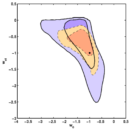
For our most general, evolving dark energy model, however, the effects of perturbations in the dark energy component are more important and neglecting them can lead to spuriously tight constraints. Figure 9 compares the results in the ($w_{\rm 0}$,$w_{\rm et}$) plane obtained when including dark energy perturbations (solid contours) or neglecting them (dashed contours). When the effects of dark energy perturbations are wrongly ignored, we obtain spuriously tight constraints on $w_{\rm 0}=-1.25^{+0.25}_{-0.34}$ and especially $w_{\rm et}=-0.67^{+0.21}_{-0.30}$; the apparent uncertainties in the latter are reduced by a factor of $\sim 2$ from the values in Table 2. Figure 9 also shows that when we incorrectly neglect the effects of dark energy perturbations, the sharp boundary provided by the CMB data set around $w_{\rm et}\sim 0$ is not reached.

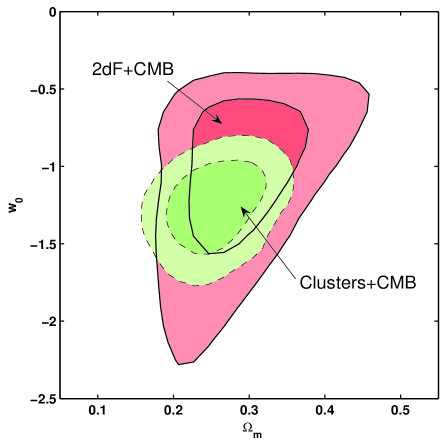
Finally it is interesting to compare the constraints on the matter content and dark energy parameters from this study with other work where the CMB and SNIa data have been combined with independent constraints from galaxy redshift surveys (e.g. Spergel et al. (2003), Tegmark et al. (2004)). The cluster X-ray gas mass fraction and galaxy redshift survey data break parameter degeneracies in the CMB data in similar ways. This is shown in Figure 10 which compares the results for a constant equation of state model using the Cluster+CMB data (green, dashed contours) or when combining the CMB data with constraints from the 2dF galaxy redshift survey (Percival et al. (2002); red, solid contours. The are the same constraints used by Spergel et al. (2003).) It is clear from the figure that the inclusion of the cluster gas fraction data leads to tighter constraints on $\Omega_{\rm m}$ and, especially, $w_{\rm 0}$. However, when the SNIa data are also included, the constraints from the clusters+CMB+SNIa and 2dF+CMB+SNIa data sets are similar, due again to the complementary nature of the various data sets. For the 2dF+CMB+SNIa data, we obtain $w_{\rm 0}=-1.02^{+0.12}_{-0.13}$ and $\Omega_{\rm m}=0.304\pm 0.031$, which are comparable to the values in Table 1. Note that the 2dF+CMB constraints shown in Figure 10 are somewhat weaker than those presented by Spergel et al. (2003). This is due primarily to the inclusion of dark energy perturbations in the present study. Spergel et al. (2003) also employ a prior $\tau<0.3$ which has a small effect on the contours. Such a prior is not included here.

Figure 11: The 68.3 and 95.4 per cent confidence limits in the $(n_{s},\Omega_{\rm b}h^{2})$ plane from the analyses of SNIa+CMB data (left panel) and clusters+CMB data (right panel) using the dark energy model with $z_{\rm t}=0.35$. Also shown are the thinned samples, where the colours correspond to the value of $\tau$. Note how the combination of clusters+CMB data alleviates the degeneracies between these parameters.

Figure 12: The 68.3 and 95.4 per cent confidence limits in the $(\Omega_{\rm m},w_{\rm 0})$ planes from the analysis of all three data sets combined, assuming either a flat prior (solid contours) or including the curvature as an additional free parameter (dashed contours). The left panel shows the results for constant $w$ and the right panel for a the $z_{\rm t}=1$ dark energy model.

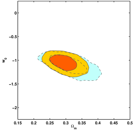
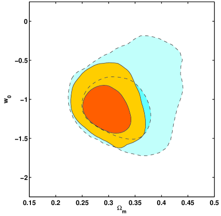
Using our most general dark energy model, we find that the combination of 2dF+SNIa+CMB data leads to slightly weaker and more negative values for $w_{\rm 0}$ and larger values for $w_{\rm et}$, which rule out the cosmological constant at 1$\sigma$. However, as discussed above, the departure from the cosmological constant becomes insignificant when we also include the cluster gas fraction data.

5 Discussion

In this paper, we have examined the evolution of dark energy using a combination of three cosmological data sets: CMB anisotropies, SNIa and the gas fraction in X-ray luminous galaxy clusters. Employing a minimum of prior information, we have obtained tight constraints on various key parameters including the dark energy equation of state. Assuming that the equation of state remains constant with time, and assuming a flat prior, we measure $w_{\rm 0}=-1.05^{+0.10}_{-0.12}$. Employing a series of more general dark energy models, we find no significant evidence for evolution in the equation of state. A cosmological constant is a good description of the current data. For models other than a cosmological constant, we have included the effects of perturbations in the dark energy component to avoid violating energy–momentum conservation. We have shown that neglecting perturbations can lead to spuriously tight constraints on dark energy models, especially for the $w_{\rm et}$ parameter (by up to a factor two for our most general model).

Although each of the data sets used here probes certain aspects of dark energy by itself, much tighter constraints are obtained when the data are combined. The SNIa and cluster data provide the primary source of information on the evolution of dark energy. Of these, the SNIa data currently contribute the stronger constraints. However, this power can only be utilised once a tight constraint on $\Omega_{\rm m}$, in this case provided by the combination of the cluster+CMB (or cluster+BBN+HST) data, is included. Using the SNIa data alone, one is hampered by a degeneracy between the equation of state $w$ and $\Omega_{\rm m}$ e.g. Riess et al. (2004) (see also Wang & Tegmark (2004)). This is the reason that some authors have employed a strong prior on $\Omega_{\rm m}$ in their studies using SNIa data (Alam et al., 2004; Jassal, Bagla, & Padmanabhan, 2004; Jonsson et al., 2004; Jain, Alcaniz, & Dev, 2004); without such a prior, the SNIa data alone cannot provide tight constraints on even constant equation of state models, much less models with evolution in $w$. Rather than introducing strong priors, our approach has been to use a combination of data sets that are complementary in nature and which allow certain key parameter degeneracies to be broken.

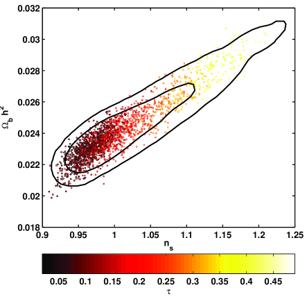
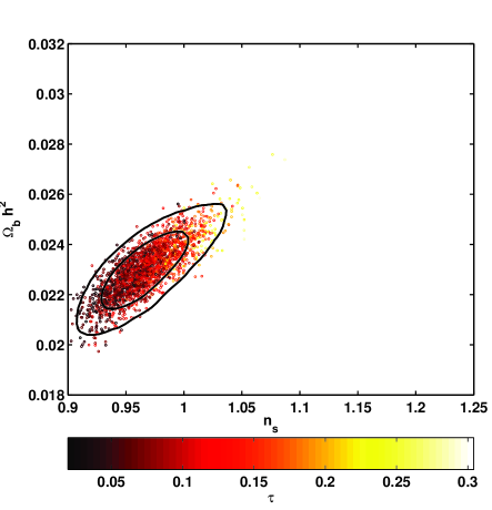
One of the main parameter degeneracies highlighted in previous studies (Corasaniti et al., 2004) is between the scalar spectral index $n_{s}$, the physical baryon density $\Omega_{\rm b}h^{2}$ and the optical depth to reionisation, $\tau$; this degeneracy impinges on the measured dark energy parameters. As noted by Corasaniti et al. (2004), the integrated Sachs-Wolfe effect in the case of an evolving dark energy equation of state increases the importance of this degeneracy with respect to constant $w$ models. The left panel of Fig 11 shows this degeneracy for the case of the SNIa+CMB data, using the $z_{\rm t}=0.35$ dark energy model. The right panel shows how the degeneracy is lessened when the clusters+CMB data are used. The combination of clusters+CMB data also leads to a tight constraint on $H_{0}$ (e.g. Allen et al. (2003)).

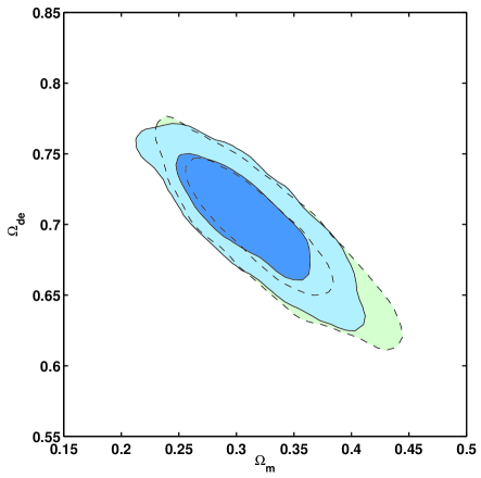
The combination of clusters+CMB data even allows us to relax the assumption that the Universe is flat, although we note that the computation of MCMC chains in the non-flat case is time consuming when one wishes to ensure convergence with $R-1<0.1$. (For this reason, we have only carried out a limited exploration of non-flat models here.) In order to avoid unphysical regions of the parameter space when using non-flat models, we have also included a prior on the optical depth to reionisation, $\tau<0.3$, in a similar manner to WMAP team (Spergel et al., 2003) and Corasaniti et al. (2004). Figure 12 shows the 68.3 and 95.4 per cent confidence limits in the ($\Omega_{\rm m}$,$w_{\rm 0}$) plane obtained assuming a constant dark energy equation of state (left panel) and using the $z_{\rm t}=1$ model (right panel), with (dashed lines) and without (solid lines) the curvature included as a free parameter. Comparison of the curves shows that the uncertainties in the parameters are increased when the assumption of flatness is dropped. However, we still have clear evidence that $w_{\rm 0}<-1/3$ and therefore that the Universe is accelerating at late times. For the constant equation of state model, we obtain tight constraints on $\Omega_{\rm k}=-0.017^{+0.020}_{-0.021}$, $\Omega_{\rm m}=0.314^{+0.040}_{-0.036}$ and $\Omega_{\rm de}=0.703^{+0.026}_{-0.030}$. The median parameter values and parameter values at the peaks of the marginalised probability distributions (and 68 per cent confidence intervals) for $w_{\rm 0}$, $w_{\rm et}$ and $\Omega_{\rm m}$ using the non-flat models are summarised in Table 2. Figure 13 shows the results in the ($\Omega_{\rm m}$,$\Omega_{\rm de}$) plane.

Finally, it is encouraging to recognise the prospects for advances in this work over the next $1-2$ years. Further Chandra observations of X-ray luminous, high-redshift, dynamically relaxed clusters should lead to rapid improvements in the constraints from the X-ray method. Continual progress in SNIa studies is expected over the next few years and the forthcoming, second release of WMAP data should, at the very least, provide an important, overall tightening of the constraints. In the long term, the combination of complementary constraints from missions such as Constellation-X, SNAP and Planck, combining high precision with a tight control of systematic uncertainties, offers our best prospect for understanding the nature of dark energy.

Figure 13: The 68.3 and 95.4 per cent confidence limits in the $(\Omega_{\rm m}$,$\Omega_{\rm de})$ plane from the analysis of the combined cluster+SNIa+CMB data set, with $\Omega_{k}$ included as a free parameter. The solid contours show the constraints for constant $w$. The dashed contours show the results for the $z_{\rm t}=1$ dark energy model.

References

- Alam et al. (2004) Alam U., Sahni V., Starobinsky, A. A., 2004, JCAP, 0406, 008
- Allen et al. (2004) Allen S. W., Schmidt R. W., Ebeling H., Fabian A. C., van Speybroeck L., 2004, MNRAS, 353, 457
- Allen et al. (2003) Allen S. W., Schmidt R. W., Bridle S. L., 2003, MNRAS, 346, 593
- Astier (2001) Astier P., 2001, Physics Letters B, 500, 8
- Armendariz–Picon et al. (2000) Armendariz–Picon C., Mukhanov V., Steinhardt P. J., 2000, Phys. Rev. Lett. 85, 4438
- Bassett et al. (2004) Bassett B. A., Corasaniti P. S., Kunz M., 2004, preprint (astro-ph/0407364)
- Bean et al. (2001) Bean R., Hansen S. H., Melchiorri A., 2001, Phys. Rev.D, 64, 103508
- Caldwell et al. (1998) Caldwell R., Dave R., Steinhardt P., 1998, Phys. Rev. Lett., 80, 1582
- Caldwell (2002) Caldwell R. R., 2002, Physics Letters B, 545, 23
- Caldwell & Doran (2005) Caldwell R. R., Doran M., 2005, preprint (astro-ph/0501104)
- Carroll et al. (2003) Carroll S. M., Hoffman M., Trodden M., 2003, Phys. Rev.D, 68, 023509
- Chevallier & Polarski (2001) Chevallier M., Polarski D., 2001, Int. J. Mod. Phys., D10, 213
- Corasaniti et al. (2003) Corasaniti P. S., Bassett B. A., Ungarelli C., Copeland E. J., 2003, Phys. Rev. Lett., 90, 091303
- Corasaniti et al. (2004) Corasaniti P. S., Kunz M., Parkinson D., Copeland E. J., Bassett B. A., 2004, Phys. Rev.D, in press (astro-ph/0406608)
- Efstathiou (1999) Efstathiou G., 1999, MNRAS, 310, 842
- Ferreira & Joyce (1998) Ferreira P., Joyce M., 1998, Phys. Rev.D, 58, 023503
- Freedman et al. (2001) Freedman W., et al., 2001, ApJ, 553, 47
- Gelman & Rubin (1992) Gelman A., Rubin D. B., 1992, Statist. Sci., 7, 457
- Hinshaw et al. (2003) Hinshaw G., et al., 2003, ApJ S., 148, 135
- Hu (2004) Hu W., 2004, preprint (astro-ph/0410680)
- Huterer & Turner (1999) Huterer D., Turner M. S., 1999, Phys. Rev.D, 60, 081301
- Jain, Alcaniz, & Dev (2004) Jain D., Alcaniz J. S., Abha D., 2004, preprint (astro-ph/0409431)
- Jassal, Bagla, & Padmanabhan (2004) Jassal H. K., Bagla J. S., Padmanabhan T., 2004, preprint (astro-ph/0404378)
- Jonsson et al. (2004) Jonsson J., Goobar A., Amanullah R., Bergstrom L., 2004, preprint (astro-ph/0404468)
- Kirkman et al. (2003) Kirkman D., Tytler D., Suzuki N., O’Meara J. M., Lubin D., 2003, ApJ S., 149, 1
- Knop et al. (2003) Knop R. A., et al., 2003, ApJ, 598, 102
- Kogut et al. (2003) Kogut A., et al., 2003, ApJ S., 148, 161
- Kuo et al. (2004) Kuo C. L., et al., 2004, Astrophys. J., 600, 32
- Lewis & Bridle (2002) Lewis A., Bridle S., 2002, Phys. Rev.D, 66, 103511
- Lewis et al. (2000) Lewis A., Challinor A., Lasenby A., 2000, Astrophys. J., 538, 473
- Linder (2003) Linder E. V., 2003, Phys. Rev. Lett., 90, 091301
- Maor et al. (2001) Maor I., Brustein R., Steinhardt P. J., 2001, Phys. Rev. Lett., 86, 6
- Pearson et al. (2003) Pearson T. J., et al., 2003, Astrophys. J., 591, 556
- Peebles & Ratra (1988) Peebles P., Ratra B., 1988, ApJ, 325, L17
- Percival et al. (2002) Percival W.J., et al., 2002, MNRAS, 337, 1068
- Perlmutter et al. (1999) Perlmutter S., et al., 1999, ApJ, 517, 565
- Rapetti & Weller (2005) Rapetti D., Weller J., 2005, to be published
- Ratra & Peebles (1988) Ratra B., Peebles P., 1988, Phys. Rev.D, 37, 3406
- Riess et al. (1998) Riess A., et al., 1998, Astron. J, 116, 1009
- Riess et al. (2004) Riess A. G., et al., 2004, ApJ, 607, 665
- Saini et al. (2000) Saini T. D., Raychaudhury S., Sahni V., Starobinsky A. A., 2000, Phys. Rev. Lett., 85, 1162
- Spergel et al. (2003) Spergel D. N., et al., 2003, ApJ S., 148, 175
- Verde et al. (2003) Verde L., et al., 2003, ApJ S., 148, 195
- Wang & Tegmark ( 2004) Wang Y., Tegmark M., 2004, Phys. Rev. Lett., 92, 241302
- Tegmark et al. ( 2004) Tegmark M., et al, 2004, Phys. Rev.D, 69, 103501
- Weller & Albrecht ( 2001) Weller J., Albrecht A., 2001, Phys. Rev. Lett., 86, 1939
- Weller & Albrecht ( 2002) Weller J., Albrecht A., 2002, Phys. Rev.D, 65, 103512
- Weller & Lewis (2003) Weller J., Lewis A. M., 2003, MNRAS, 346, 987
- Wetterich (1988) Wetterich C., 1988, Nucl. Phys., B302, 668
- Zlatev et al. (1999) Zlatev I., Wang L. M., Steinhardt P. J., 1999, Phys. Rev. Lett., 82, 896