Least-Squares methods with Poissonian noise: an
analysis and a comparison with the Richardson-Lucy algorithm

It is well-known that the noise associated with the collection of an astronomical image by a CCD camera is, in large part, Poissonian. One would expect, therefore, that computational approaches that incorporate this a priori information will be more effective than those that do not. The Richardson-Lucy (RL) algorithm, for example, can be viewed as a maximum-likelihood (ML) method for image deblurring when the data noise is assumed to be Poissonian. Least-squares (LS) approaches, on the other hand, arises from the assumption that the noise is Gaussian with fixed variance across pixels, which is rarely accurate. Given this, it is surprising that in many cases results obtained using LS techniques are relatively insensitive to whether the noise is Poissonian or Gaussian. Furthermore, in the presence of Poisson noise, results obtained using LS techniques are often comparable with those obtained by the RL algorithm. We seek an explanation of these phenomena via an examination of the regularization properties of particular LS algorithms. In addition, a careful analysis of the RL algorithm yields an explanation as to why it is more effective than LS approaches for star-like objects, and why it provides similar reconstructions for extended objects. We finish with a convergence analysis of the RL algorithm. Numerical results are presented throughout the paper. It is important to stress that the subject treated in this paper is not academic. In fact, in comparison with many ML algorithms, the LS algorithms are much easier to use and to implement, often provide faster convergence rates, and are much more flexible regarding the incorporation of constraints on the solution. Consequently, if little to no improvement is gained in the use of an ML approach over an LS algorithm, the latter will often be the preferred approach.

1 Introduction

The restoration of images is a common problem in Astronomy. Astronomical images are blurred due to several factors: the refractive effects of the atmosphere, the diffractive effects of the finite aperture of the telescope, the statistical fluctuations inherent in the collection of images by a CCD camera, and instrumental defects. An illuminating example is represented by the spherical aberration of the primary mirror of the Hubble Space Telescope (White 1991) that limited the quality of the images before the detector system was refurbished.

The widespread interest in this subject has resulted in the development of a large number of algorithms with different degrees of sophistication (for a review, see Starck et al, 2002). For example, recent wavelet-based approaches have been shown to provide excellent results (e.g., see Neelamani et al. 2004). Unfortunately, these algorithms are very expensive to implement, prohibiting their use on large-scale image restoration problems and on problems that require the restoration of a large number of images. Consequently, for many restoration problems, less sophisticated and computationally more efficient algorithms must be used. In this respect, the algorithms based on a linear Least-Squares (LS) methodology represent an interesting class. In this paper we discuss two LS approaches: direct and iterative. Direct methods, which we discuss in Sec. 3.1, are the most computationally efficient, while iterative techniques, which we discuss in Sec. 3.2, allow for the straightforward incorporation of constraints.

In spite of the beneficial characteristics of the LS-based algorithms, astronomers typically use techniques based on a non-linear approach. Such algorithms are usually more difficult to implement, are less flexible and often have slow convergence rates. In particular, the original Richardson-Lucy (RL) algorithm (Richardson 1972; Lucy 1974; Shepp & Vardi 1982) and later modifications have seen a great deal of attention. RL can be viewed as an Expectation-Maximization (EM) algorithm associated with a Poisson statistical noise model. Linear LS methods, on the other hand, can be viewed as the maximum-likelihood (ML) approach when the noise contaminating the image(s) of interest is additive Gaussian with constant variance across pixels. For CCD camera noise, the statistical assumption inherent in the RL algorithm is much more accurate than that of the LS approach (see Sect. 2). Nonetheless, it is often the case that these two methods provide results of similar quality (see Sec. 4). From a particular point of view, this fact is disappointing, since it means that in certain instances the RL algorithm is not able to exploit the a priori statistical information. This is particularly relevant when the incorporation of the a priori information results in algorithms that are more expensive and difficult to implement.

The aims of the present paper are as follows: I) to determine the performance of the LS algorithms when the noise is predominantly Poissonian; II) to determine when the LS and RL approaches will give very similar qualitative results. We stress that such questions are not only of academic interest. In fact, the authors believe that due to certain distinct computational advantages, the LS algorithms should be used whenever their use is warranted. On the other hand, we caution that it is not our intention to conclude that the LS approach is always the best choice. In fact, as we will show, this is not the case.

In the next section, we present the statistical model for CCD camera image formation as well as the approximate model that we will use in the paper. After some preliminary considerations in Sec. 2, in Sec. 3 we will explore the convergence properties of two LS approaches. We will also discuss the performance of these algorithms on different objects. Finally, in Sec. 4 we will explore in detail the convergence properties the RL algorithm. Throughout the paper we will present numerical results. Finally, we present our conclusion in Section 5.

2 Statistical Considerations

Astronomical image data is typically collected with a device known as a CCD camera. The following statistical model (see Snyder et. al 1993, 1995) applies to image data from a CCD detector array:

$$b(i,j)=n_{\rm obj}(i,j)+n_{\rm bck}(i,j)+n_{\rm rdn}(i,j).$$ (1)

Here, $b(i,j)$ is the data acquired by a readout of the pixels of the CCD detector array; $i,j=1,2,\dots,N$ (without loss of generality, square images are considered); $n_{obj}(i,j)$ is the number of object dependent photoelectrons; $n_{\rm bck}(i,j)$ is the number of background electrons; and $n_{\rm rdn}(i,j)$ is the readout noise. The random variables $n_{\rm obj}(i_{1},j_{1})$, $n_{\rm bck}(i_{1},j_{1})$, and $n_{\rm rdn}(i_{1},j_{1})$ are assumed to be independent of one another and of $n_{\rm obj}(i_{2},j_{2})$, $n_{\rm bck}(i_{2},j_{2})$, and $n_{\rm rdn}(i_{2},j_{2})$ for $i_{1},j_{1}\neq i_{2},j_{2}$.

For clearness of presentation, it is helpful to use matrix-vector notation. We rewrite Eq. (1) as

$$\boldsymbol{b}=\boldsymbol{n}_{\rm obj}+\boldsymbol{n}_{\rm bck}+\boldsymbol{n}_{\rm rdn},$$ (2)

where the vectors have been obtained by column stacking the corresponding two-dimensional arrays. The random vector $\boldsymbol{n}_{\rm obj}$ has a Poisson distribution with Poisson parameter $\boldsymbol{A}\boldsymbol{x}$, where $\boldsymbol{x}$ is the true image, or object, and $\boldsymbol{A}$ is a matrix that corresponds to the point spread function (PSF). Depending upon the assumed boundary conditions, its structure is typically block-circulant or block-Toeplitz (e.g., see Vio et al. 2003; Vogel 2002); $\boldsymbol{n}_{bck}$ is a Poisson random vector with a fixed positive Poisson parameter $\beta$; and $\boldsymbol{n}_{\rm rdn}$ is a Gaussian random vector with mean $0$ and fixed variance $\sigma^{2}_{\rm rdn}$.

In the sequel, we will use the following notation to denote model (2):

$$\boldsymbol{b}={\rm Poisson}[\boldsymbol{A}\boldsymbol{x}]+{\rm Poisson}[\beta\cdot\boldsymbol{1}]+\boldsymbol{N}_{(0,\sigma_{rdn}^{2})},$$ (3)

where ${\rm Poisson}[\boldsymbol{\mu}]$ denotes a Poissonian random vector with mean $\boldsymbol{\mu}$, whereas $\boldsymbol{N}_{(\boldsymbol{\mu},\boldsymbol{\sigma}^{2})}$ represents a Gaussian random vector with mean $\boldsymbol{\mu}$ and variance $\boldsymbol{\sigma}^{2}$ (for iid entries, $\boldsymbol{\mu}=\mu$ and $\boldsymbol{\sigma}^{2}=\sigma^{2}$). If $\sigma_{\rm rdn}^{2}$ is large, we have ${\rm Poisson}[\sigma^{2}_{\rm rdn}]\approx N_{(\sigma^{2}_{\rm rdn},\sigma^{2}_{\rm rdn})}$ (see Feller 1971), and hence, using the independence properties of the random variables in Eq. (1) we obtain the following approximation of Eq. (3):

$$\boldsymbol{b}={\rm Poisson}[\boldsymbol{A}\boldsymbol{x}+\boldsymbol{1}\cdot(\beta+\sigma^{2}_{\rm rdn})]-\sigma^{2}_{\rm rdn}.$$ (4)

In order to simplify the analysis that follows, we assume the following simplified model

$$\boldsymbol{b}={\rm Poisson}[\boldsymbol{A}\boldsymbol{x}].$$ (5)

The analysis is easily extended to the model given by Eq. (4). Furthermore, in regions of high intensity $\boldsymbol{A}\boldsymbol{x}\gg\beta,\sigma^{2}$, in which case model (4) is well-approximated by model (5).

A further useful approximation is possible if the elements of $\boldsymbol{b}$ are large. In fact, in this case model (5) can be well approximated with

$$\boldsymbol{b}=\boldsymbol{A}\boldsymbol{x}+\boldsymbol{z},$$ (6)

where $\boldsymbol{z}$ is a zero mean Gaussian random vector

$$\boldsymbol{z}\approx\boldsymbol{\gamma}\odot\boldsymbol{N}_{(0,1)}.$$ (7)

Here symbol “$\leavevmode\nobreak\ \odot\leavevmode\nobreak\$” denotes Hadamard (element-wise) multiplication, and $\boldsymbol{\gamma}=(\boldsymbol{A}\boldsymbol{x})^{1/2}$. In other words, through (6), the nonlinear noise model (5) can be approximated with a linear, additive, nonstationary, Gaussian noise model. Our own numerical experiments suggest that $b_{i}>40$ is sufficient. This condition is true in many situations of practical interest (recall that $b_{i}$ is the number of photons detected by the $i$th pixel in the CCD camera).

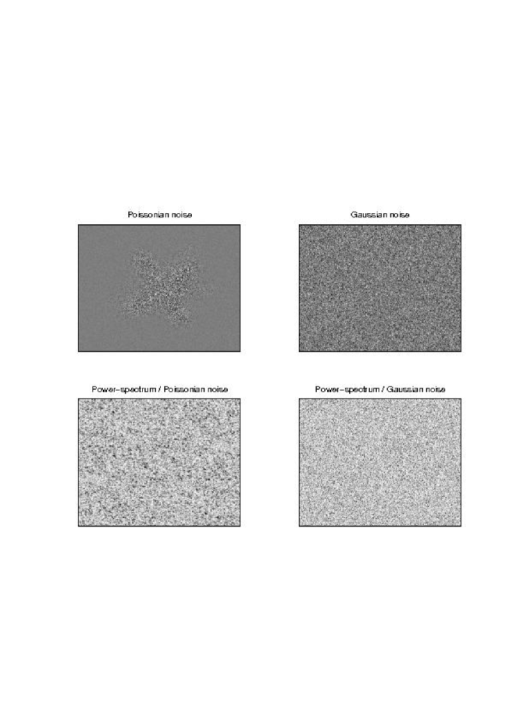
From equations (6) and (7) we see that $\boldsymbol{z}$ has a flat spectrum, i.e., the expected modulus of its Discrete Fourier Transform (DFT) is constant. However, here, at difference with a gaussian white noise process, the various Fourier frequencies are not independent from one another (e.g., see Fig. 1). The reason is that the point-wise multiplication in the spatial domain corresponds to convolution in the Fourier domain, and vice versa. Thus, from (7), we have

$$\widehat{z}(i,j)=[\widehat{\gamma}\otimes\widehat{N}_{(0,1)}](i,j),$$ (8)

where the symbol “$\leavevmode\nobreak\ \widehat{}\leavevmode\nobreak\$” indicates DFT, “$\leavevmode\nobreak\ \otimes\leavevmode\nobreak\$” denotes convolution, and $(i,j)$ represents a two-dimensional, discrete frequency index. Since convolution is a linear operation, and $\{\widehat{N}_{(0,1)}(i,j)\}$ are iid complex Gaussian random variables with zero mean and unit variance, $\{\widehat{z}(i,j)\}$ are complex Gaussian random variables with zero mean and a constant variance equal to $\sum_{i,j}|\widehat{\gamma}(i,j)|^{2}$.

3 Performance of the Least-Squares Approach

The fact that the noise process $\boldsymbol{z}$ has a flat spectrum, provides some insight into the performance of the LS deblurring algorithms in presence of Poissonian noise. In particular, since the LS approach corresponds to the assumption that the contaminating noise is an additive white noise process, the possible worsening of the performance of LS algorithms has to be expected due to their inability to take into account the dependence between the Fourier frequencies that characterize the spectrum of $\boldsymbol{z}$. The question then arises, what happens if such dependence is not taken into account? The following two arguments suggest that, in many astronomical applications, the consequences are not so important:

1. images of astronomical interest have spectra in which only the lowest frequencies have intensities that are remarkably different from zero. This is a consequence of the fact that the PSFs are nearly band limited, i.e, they are very smooth functions. Furthermore, if a function is in $\boldsymbol{{\mathrm{C}}}^{k}$ (i.e., it has $k$ continuous derivatives) then its spectrum decreases at least as fast as $1/\nu^{k+1}$. Consequently, this constitutes the lower-limit with which the spectrum of the images can be expected to decrease;

2. The discrete Picard’s condition plus the Riemann-Lebesgue lemma (Hansen 1997) show that the only Fourier frequencies useful for the restoration of the image are (roughly) those where the contribution of the object is larger than that of the noise.

From such considerations, it is possible to conclude that in the construction of the deblurred image only a few frequencies (i.e., the lowest ones) are primarily used, whereas most of the remaining frequencies are of only marginal importance. For example, in the case of a star-like source (i.e., a non-bandlimited function) and Gaussian PSF with circular symmetry (a $\boldsymbol{{\mathrm{C}}}^{\infty}$ function) and dispersion (in pixels) $\sigma_{p}$, the observed spectrum is again a Gaussian function with circular symmetry and dispersion (in pixels) $\widehat{\sigma}_{p}$ given by:

$$\widehat{\sigma}_{p}\approx N/(2\pi\sigma_{p}).$$ (9)

In several of the numerical experiments presented below, we have used $N=256$ and $\sigma_{p}=12$. In this case, $\widehat{\sigma}_{p}\approx 3.5$. With the levels used in the simulations, it happens that in $\widehat{b}(i,j)$, the noise becomes dominant when (approximately) $i,j\geq\gamma$, where $10\leq\gamma\leq 20$ corresponding to different noise levels. Hence, the LS algorithms can be expected to be almost insensitive to the nature of the noise.

Another point worth noting is that, although the set of frequencies most corrupted by noise are determined both by the noise level and by the spectrum of the PSF, it is the latter factor that has the most influence. To see this we note that, for the case of the star-like source and Gaussian PSF considered above, it is possible to show that the frequency index $(i,j)$ where the spectrum of the signal and that of $\boldsymbol{z}$ have the same level is given by $r\approx N\sqrt{\ln(A_{s}/\sigma_{\boldsymbol{z}})}/(\pi\sigma_{p}\sqrt{2})$, where $r=(i^{2}+j^{2})^{1/2}$, $A_{s}$ is the amplitude of the source, and $\sigma_{\boldsymbol{z}}$ is the level of the noise spectrum.

In the next two sections, we will check the reliability of the above arguments in the context of two LS algorithms.

3.1 The Tikhonov Approach

The linear systems that one encounters when solving image restoration problems are often highly ill-conditioned. Because of this, solutions can be extremely unstable. One of the most standard approaches for handling this difficulty is known as Tikhonov regularization. In the Tikhonov approach, one obtains a stable estimate of the solution of the linear system of interest by solving the penalized least squares problem

$$\boldsymbol{x}_{\lambda}={\rm argmin}\left(\,\|\,\boldsymbol{A}\boldsymbol{x}-\boldsymbol{b}\,\|_{2}^{2}+\lambda^{2}\|\,\boldsymbol{x}\,\|_{2}^{2}\,\right),$$ (10)

or, equivalently, by solving the linear system

$$(\boldsymbol{A}^{T}\boldsymbol{A}+\lambda^{2}\boldsymbol{I})\boldsymbol{x}=\boldsymbol{A}^{T}\boldsymbol{b}.$$ (11)

Here $\lambda$ is a positive scalar known as the regularization parameter. The direct solutions of (11) can be obtained very efficiently using fast implementations of the DFT. Moreover, there are various reliable and well tested criteria that allow for the estimation of $\lambda$. A standard technique is known as the generalized cross-validation (GCV) method. With this approach, the optimal value of $\lambda$ is estimated via the minimization of the GCV function

$${\rm GCV}(\lambda)=\frac{||\boldsymbol{A}\boldsymbol{x}_{\lambda}-\boldsymbol{b}||^{2}_{2}/N^{2}}{[\,{\rm trace}(\boldsymbol{I}-\boldsymbol{{\cal A}}(\lambda))/N^{2}\,]^{2}}.$$ (12)

Here $\boldsymbol{{\cal A}}$ is the matrix that defines the estimator of $\boldsymbol{A}\boldsymbol{b}$, i.e., $\boldsymbol{{\cal A}}\boldsymbol{b}=\boldsymbol{A}\boldsymbol{x}_{\lambda}$, and $N^{2}$ is the number of pixels in the image. For Tikhonov regularization

$$\boldsymbol{{\cal A}}(\lambda)=\boldsymbol{A}(\boldsymbol{A}^{T}\boldsymbol{A}+\lambda^{2}\boldsymbol{I})^{-1}\boldsymbol{A}^{T}\boldsymbol{b}.$$ (13)

It is useful to express model (10) and the GCV function (12) in the Fourier domain:

$$\widehat{x}_{\lambda}(i,j)=\frac{\widehat{A}^{*}(i,j)}{|\widehat{A}(i,j)|^{2}+\lambda^{2}}\widehat{b}(i,j),$$ (14)

and

$${\rm GCV}(\lambda)= N^{2}\sum_{i,j=0}^{N-1}\left|\frac{\widehat{b}(i,j)}{|\widehat{A}(i,j)|^{2}+\lambda^{2}}\right|^{2}$$

$$/\left|\sum_{i,j=0}^{N-1}\frac{1}{|\widehat{A}(i,j)|^{2}+\lambda^{2}}\right|^{2}.$$ (15)

Here, one can compute both $\widehat{x}_{\lambda}$ and the minimizer of ${\rm GCV}(\lambda)$ very efficiently.

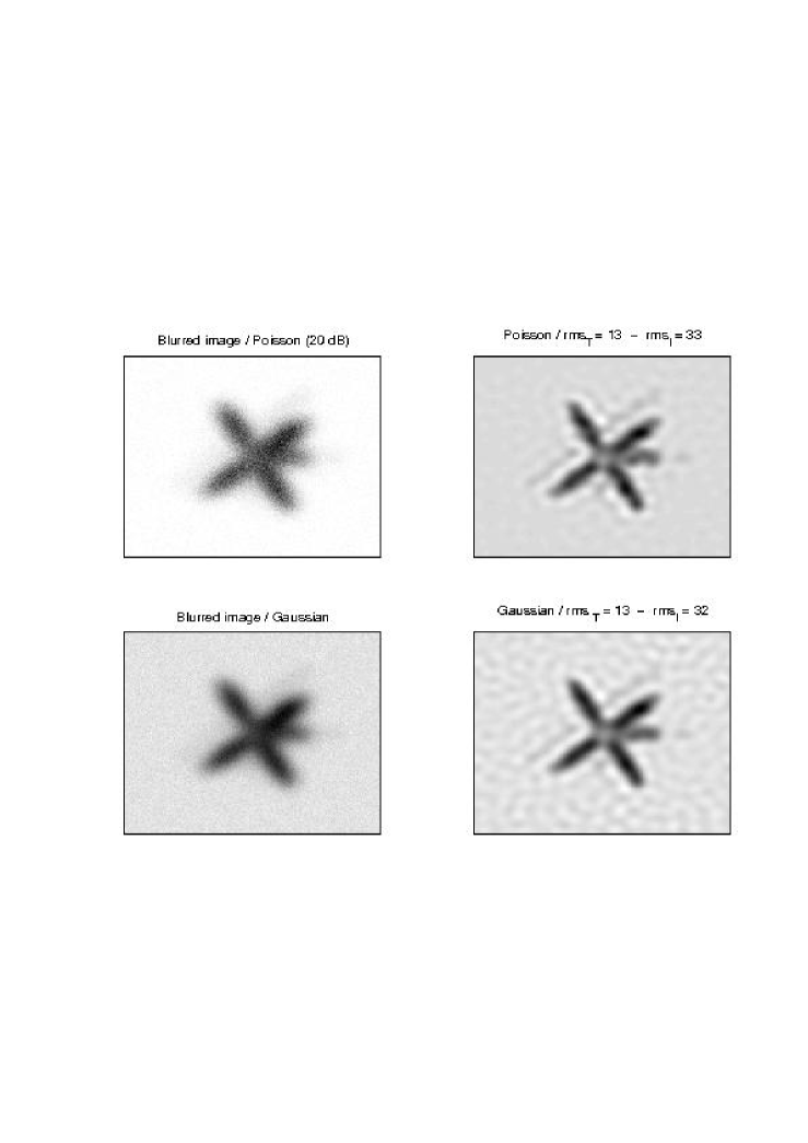
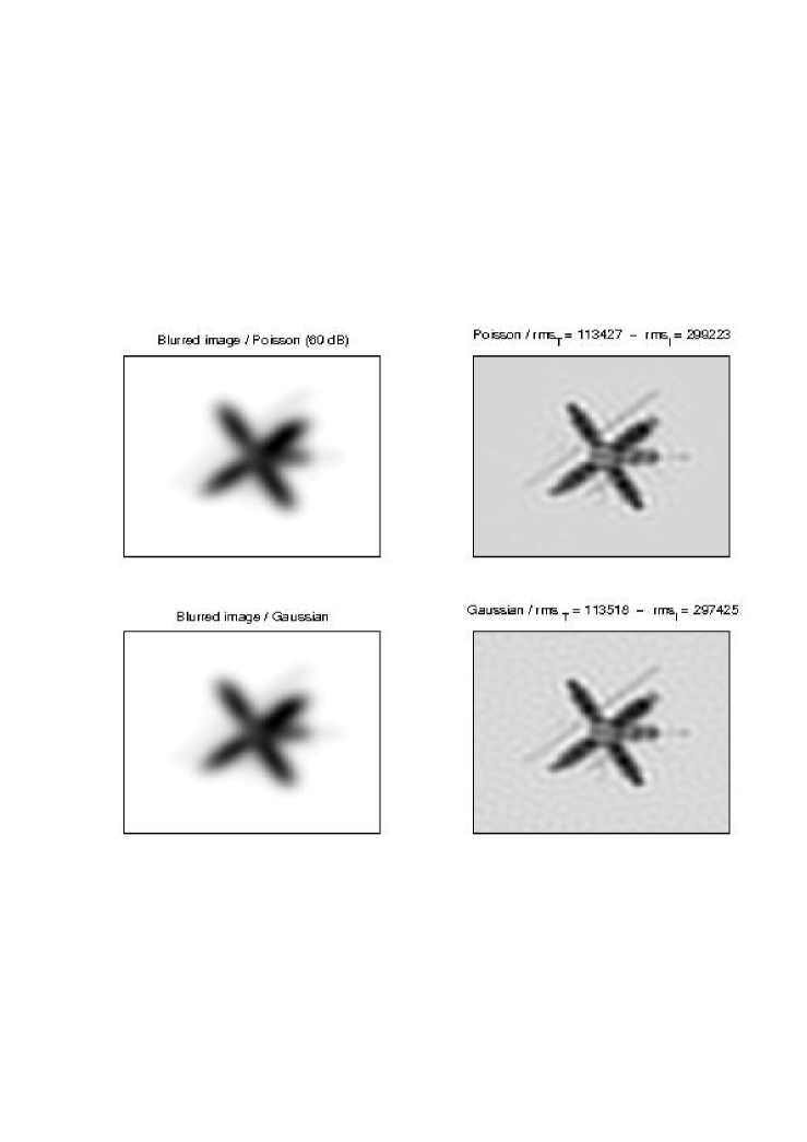
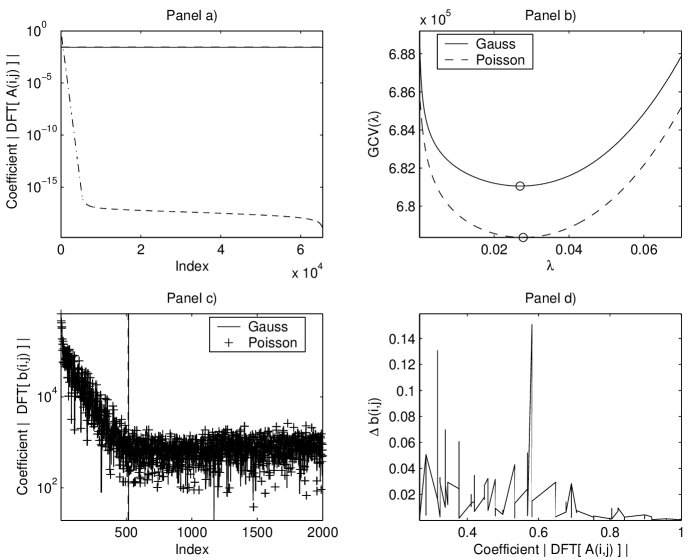
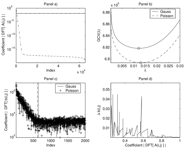
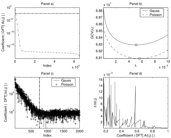
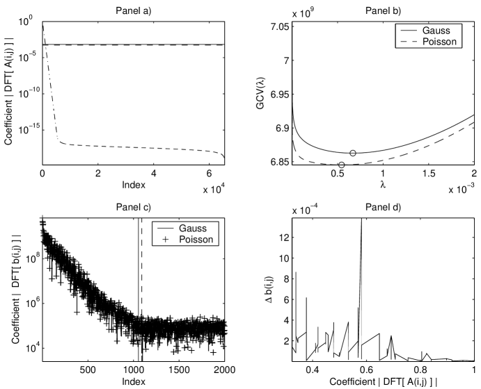
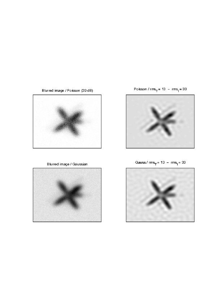
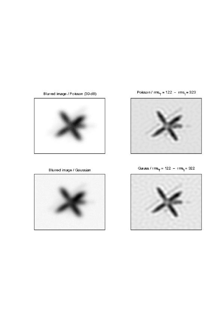
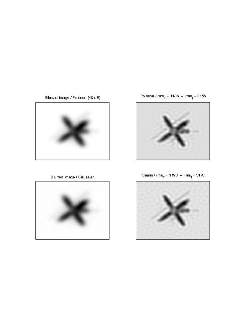
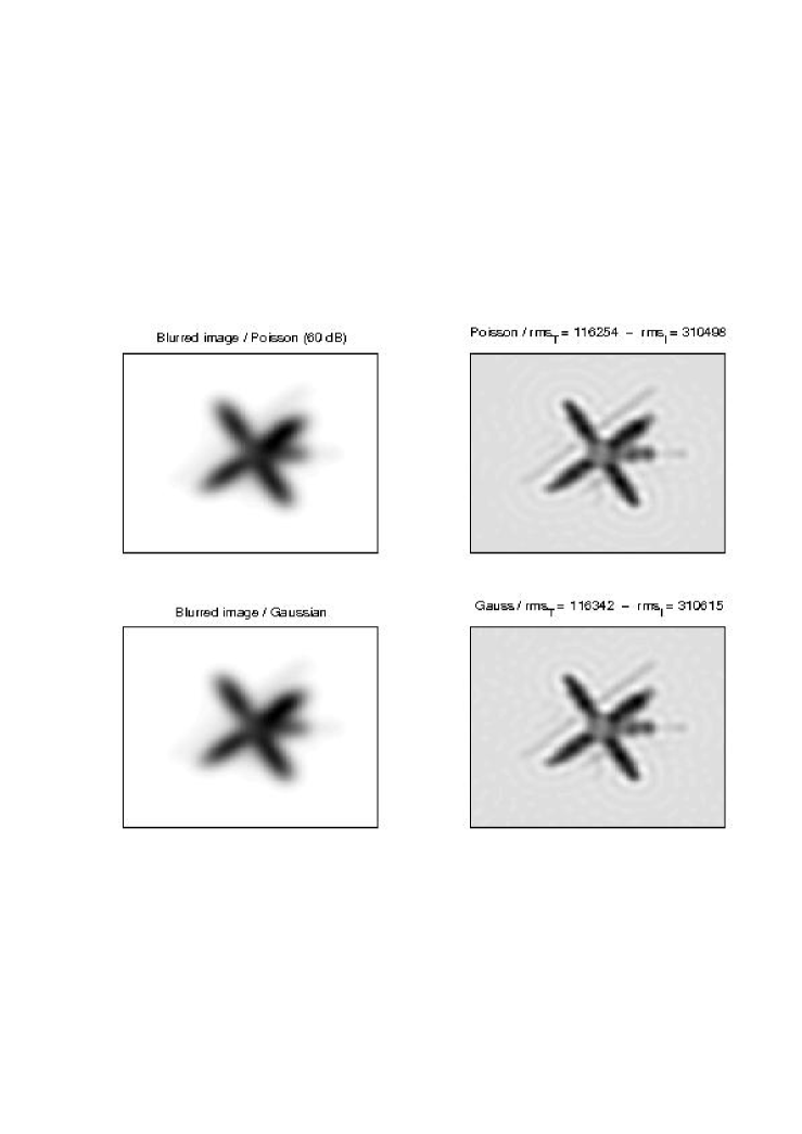
Figures 2 - 5 compare the results obtainable with this method when noises are stationary Gaussian and Poissonian, respectively. The image $b_{p}(i,j)$, contaminated by Poissonian noise, has been obtained by simulating a nonstationary Poissonian process with local mean given by the values of the pixels in the blurred images, i.e. using model (5). Four peak signal to noise (${\rm S/N}$) ratios have been considered : $20$, $30$, $40$ and $60\leavevmode\nobreak\ {\rm dB}$. They correspond to situations of very low, intermediate, and very high noise levels. The PSF used in the simulations is a two-dimensional Gaussian function with circular symmetry. The image $b_{g}(i,j)$, contaminated by Gaussian noise, has been obtained by the addition of a discrete stationary white noise process to the blurred images. Both the Gaussian and the Poissonian noises have been simulated through a classic inverse distribution method (e.g., see Johnson 1987) by transforming the same set of random uniform deviates. They have exactly the same variance. Here, the subject of interest is superimposed to a sky whose intensity, in the blurred image, is set to $1\%$ of the maximum value of the image. This means that, contrary to the Gaussian case where the noise level is constant across the image, in the Poissonian case the noise is mostly concentrated in the pixels with highest values. In spite of this fact, these figures show that the results provided by Tikhonov coupled with GCV are quite similar regardless of whether the noise is of Gaussian of Poissonian type.

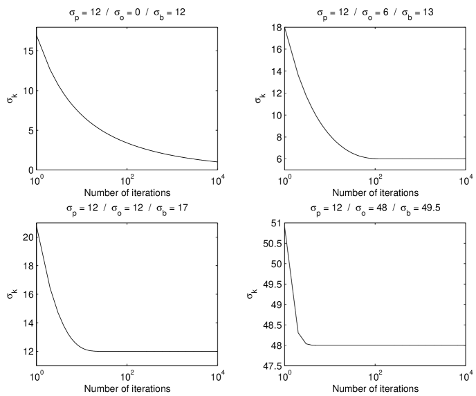
These results can be explained if one considers Eq. (14), where it is clear that the role of $\lambda$ is to replace the Fourier coefficients $\widehat{A}(i,j)$ with small modulus, i.e., those coefficients that make the deblurring operation unstable. According to the two points mentioned above, the “optimal” value of $\lambda$ should replace all the Fourier coefficients whose modulus is smaller than the expected level of the noise in the Fourier domain. Since in $b_{p}(i,j)$ and $b_{g}(i,j)$ the level of the noise is the same, such a replacement will be quite important and will have a similar effect for both images. This is shown by the results in Figs. 8 - 11. In particular, the $c)$ panels show that GCV chooses $\lambda$ so that the frequencies corresponding to the flat part of the spectra (i.e., those dominated by the noise) are filtered out. The consequence of this is that, for both Gaussian and the Poissonian noises, almost the same number of coefficients are filtered. Moreover, as is shown in the $d)$ panels, the coefficients $|\widehat{b}_{p}(i,j)|$ and $|\widehat{b}_{g}(i,j)|$ corresponding to the coefficients $\widehat{A}(i,j)$ with the largest modulus, are very similar. From this, one can conclude that the deblurred images $\boldsymbol{x}_{\lambda}$ can be expected to be very similar regardless of the nature of the noise.

The reason why the two GCV curves are almost identical (see the $b)$ panels) is that, independently from the nature of the noise, in Eq. (3.1) the quantity $\widehat{b}(i,j)$ can be replaced by $\widehat{b}(i,j)=\widehat{A}(i,j)\widehat{x}(i,j)+\widehat{z}_{n}(i,j)$, where $\widehat{z}_{n}(i,j)$ is given by Eq. (8) or by a stationary white noise process. Now, taking the expected value of the resulting ${\rm GCV}(\lambda)$, it is not difficult to show that

$${\rm E}[{\rm GCV}(\lambda)]= N^{2}\sum_{i,j=0}^{N-1}\frac{|\widehat{A}(i,j)\widehat{x}(i,j)|^{2}+\sigma^{2}_{z_{n}}}{(|\widehat{A}(i,j)|^{2}+\lambda^{2})^{2}}$$

$$/\left|\sum_{i,j=0}^{N-1}\frac{1}{|\widehat{A}(i,j)|^{2}+\lambda^{2}}\right|^{2}.$$ (16)

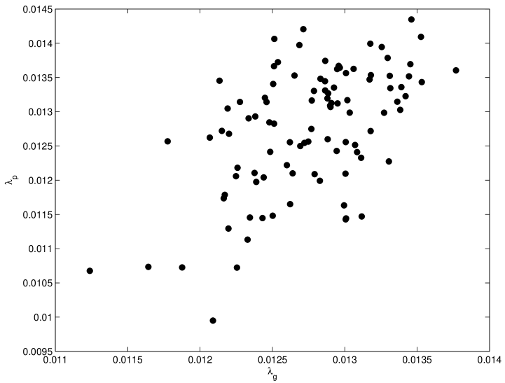
Since the term $\sigma_{z_{n}}^{2}$ is constant, the ${\rm E}[{\rm GCV}(\lambda)]$ function is independent of the specific nature of the noise. The same is not true for the variance. However, because of the arguments presented above, no instabilities are to be expected. This is supported by the fact that in our numerical experiments we have never experienced stability problems (see also Fig. 6).

3.2 The iterative approach to regularization

Iterative algorithms are commonly used in deblurring problems. Although, computationally less efficient than the direct methods, such as the Tikhonov approach discussed above, they are much more flexible in that they allow for the straightforward incorporation of constraints. These algorithms provide regularization via a semiconvergence property; that is, the iterates first reconstruct the low frequency components of the signal, i.e. those less contaminated by noise, and then the high frequency ones. In other words, the number of iterations plays the same role as the regularization parameter $\lambda$ in the Tikhonov approach.

Semiconvergence has been rigorously proved only for a limited number of algorithms. For others, some theoretical results are available but, the primary evidence stems from many years of success in use on applied problems.

The prototypical iterative algorithm for least squares problems is the Landweber method (LW). If $\boldsymbol{x}_{0}$ is the starting image (often $\boldsymbol{x}_{0}=\boldsymbol{0}$), then the iterations take the form

$$\boldsymbol{x}_{k}=\boldsymbol{x}_{k-1}+\omega\boldsymbol{A}^{T}\left[\boldsymbol{b}-\boldsymbol{A}\boldsymbol{x}_{k-1}\right],$$ (17)

where, $k=1,2,\ldots$, and $\omega$ is a real positive parameter satisfying $0<\omega<2/\|\boldsymbol{A}^{T}\boldsymbol{A}\|$. The values of $\omega$ determine, in part, the convergence of the iteration. The semiconvergence property of this algorithm is typically proved using arguments based on the singular values decomposition of the matrix $\boldsymbol{A}$ (for a discussion of this, see Vogel 2002). However, it is, perhaps, more instructive to rewrite Eq. (17) in the Fourier domain, obtaining

$$\widehat{x}_{k}(i,j)=\frac{\widehat{b}(i,j)}{\widehat{A}(i,j)}\left[1-(1-\omega|\widehat{A}(i,j)|^{2})^{k}\right],$$ (18)

with $0<\omega<2/\max\left[|\widehat{A}(i,j)|^{2}\right]$. If, as usual, the PSF is assumed to have unit volume, then $\max\left[|\widehat{A}(i,j)|^{2}\right]=1$ and $0<\omega<2$. From this equation, one can see that, for a given frequency index $(i,j)$, the closer the term $\omega|\widehat{A}(i,j)|^{2}$ is to one, the more rapid is the convergence to $\widehat{b}(i,j)/\widehat{A}(i,j)$, which corresponds to the unregularized solution. Since, as mentioned above, the largest values of the spectrum of $\widehat{A}(i,j)$ correspond to the lowest frequencies, it is evident from (18) that the lower frequencies are restored in early iterations, while progressively higher frequencies are restored as the iteration progresses.

3.2.1 Convergence properties

Equation (17) shows that the convergence of LW is driven by the rate with which the term

$$\widehat{\cal K}_{k}(i,j)=(1-\omega|\widehat{A}(i,j)|^{2})^{k}$$ (19)

goes to zero. In order to understand what this means in practical situations, it is useful to see what happens in the case of a noise-free image when the PSF is a two-dimensional Gaussian with circular symmetry and dispersion $\sigma_{p}$. Without loss of generality, we set $\omega=1$. Then

$$\widehat{\cal K}_{k}(i,j)\approx\left[1-\exp(-r^{2}/\widehat{\sigma}_{p}^{2})\right]^{k},$$ (20)

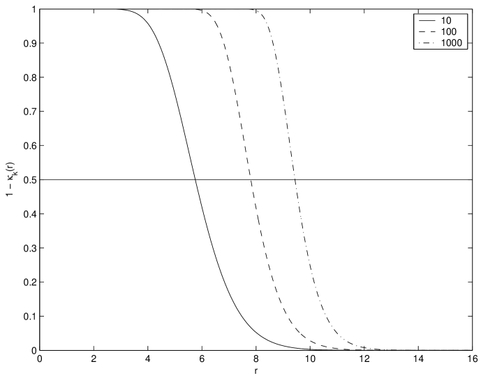
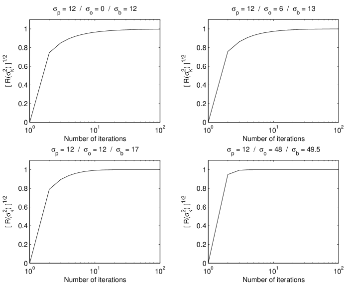
where $r^{2}=i^{2}+j^{2}$ and $\widehat{\sigma}_{p}$ is the dispersion of the PSF in the frequency domain (see Eq. (9)). From this equation, it is not difficult to see that, even in case of moderate values of $k$, the term within square brackets on the rhs of Eq. (18) can be well-approximated by the Boxcar function

$$\Pi_{k}(i,j)=\left\{\begin{array}[]{ll}1&\quad\textrm{if $0\leq|r|\leq r_{0.5,k}$};\\ 0&\quad\textrm{otherwise}\end{array}\right.,$$ (21)

where $r_{0.5,k}$ is the value of $r$ for which $\widehat{\cal K}_{k}(r)=0.5$ (see also Fig. 7). Therefore, the iterate (18) can be approximated by

$$\widehat{x}_{k}(i,j)=\frac{\widehat{b}(i,j)}{\widehat{A}(i,j)}\Pi_{k}(i,j).$$ (22)

The requirement that $\widehat{\cal K}_{k}(i,j)\leq\epsilon$, with $0<\epsilon<1$ implies

$$k>\frac{\ln\epsilon}{\ln\left[1-\exp(-r^{2}/\widehat{\sigma}_{p}^{2})\right]}.$$ (23)

This result shows that the restoration of the highest frequencies (i.e., large $r$), requires a number of iterations that becomes rapidly huge. For the case of the star-like sources, where all the frequencies have to be restored, this means a terribly slow convergence. More specifically, from Eq. (23) one can see that for frequencies $(i,j)$ such as $r\lessapprox\widehat{\sigma}_{p}$, $k\propto r$, while for larger values of $r$, $k$ increases exponentially. For example, some of the experiments presented in this paper are based on images with size $256\times 256$ pixels and with a Gaussian PSF with $\widehat{\sigma}_{p}\approx 3.5$. In this case, if $\epsilon=0.5$, in order to have $r_{0.5,k}=\widehat{\sigma}_{p},2\widehat{\sigma}_{p},3\widehat{\sigma}_{p},6\widehat{\sigma}_{p}$ (i.e., $r_{0.5,k}=3.5,7,10.5,21$), it is necessary that $k\approx 2,4,5600,3\times 10^{15}$, respectively.

The obvious conclusion is that LW is useful only for the restoration of objects for which the low-frequencies are dominant, e.g. extended objects with smooth light distributions.

3.2.2 Numerical results

Since, regardless of the noise type, LW reconstructs the lower frequency components of the image first (i.e., the frequencies where the contribution of the noise is negligible), we expect the following for both $b_{p}(i,j)$ and $b_{g}(i,j)$:

1. the resulting deblurred images should be very similar;
   

2. in early iterations the convergence rate of the algorithms should be almost identical.

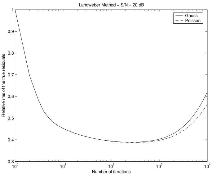
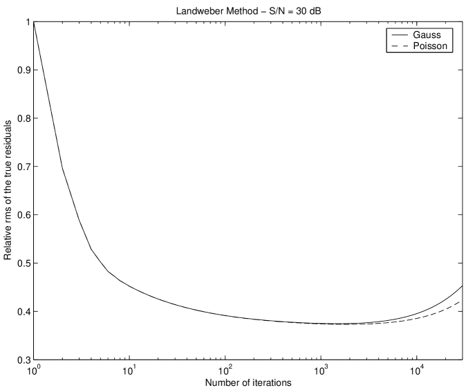
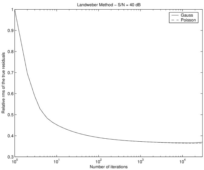
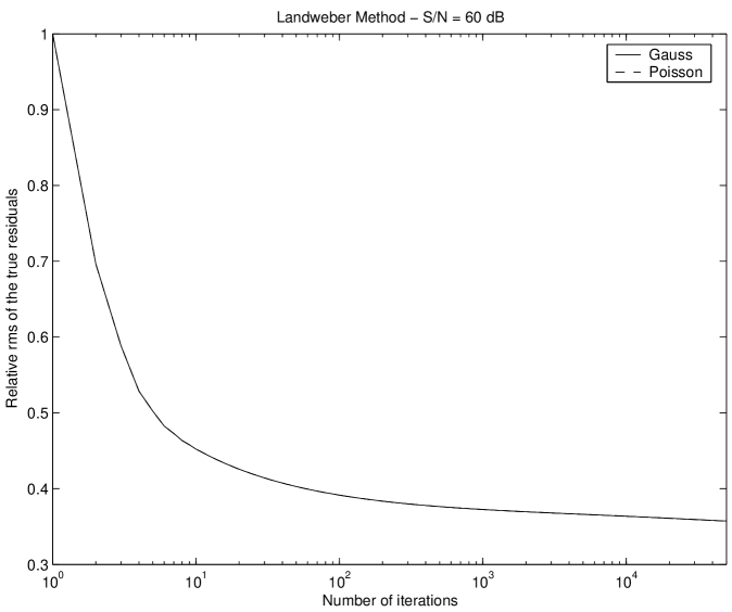
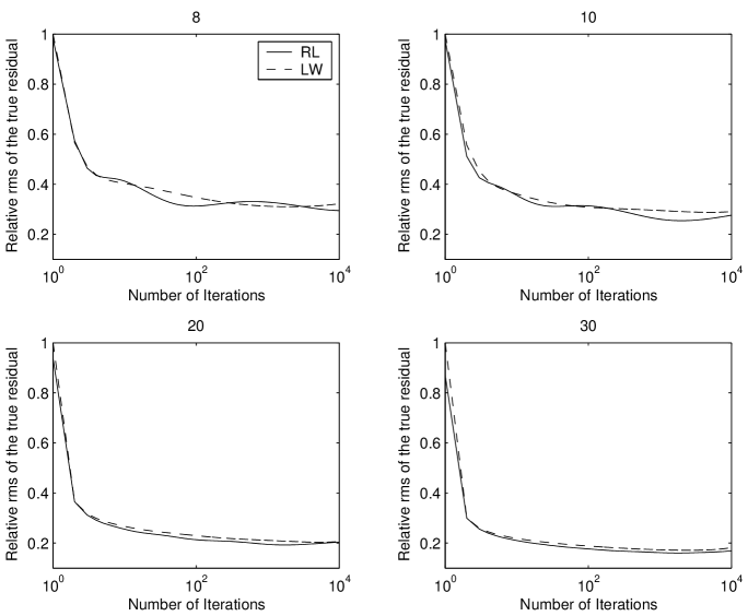
These statements are supported in Figs. 12-15 and Figs. 16-19. In particular, from the last set of figures one can see that the convergence curves are almost identical until the minimum rms of the true residual is reached. After that, because the high frequencies (the ones that are more sensitive to the nature of the noise) begin to be included in the restoration, the curves diverge.

4 Richardson-Lucy Algorithm

In the previous sections we have shown that the LS methods are relatively insensitive to the specific nature of the noise. However, this does not mean that they are optimal. In principle, methods that exploit the a priori knowledge of the statistical characteristic of the noise should be able to provide superior results.

In particular, model (5) motivates the use of the Richardson-Lucy (RL) algorithm for estimating $\boldsymbol{x}$. RL can be viewed as the EM algorithm corresponding to the statistical noise model (5). The RL algorithm is defined by the iteration

$$\boldsymbol{x}_{k+1}=\boldsymbol{x}_{k}\odot\boldsymbol{A}^{T}\frac{\boldsymbol{b}}{\boldsymbol{b}_{k}},$$ (24)

where $\boldsymbol{b}_{k}=\boldsymbol{A}\boldsymbol{x}_{k}$, and the fraction of two vectors denote Hadamard (component-wise) division.

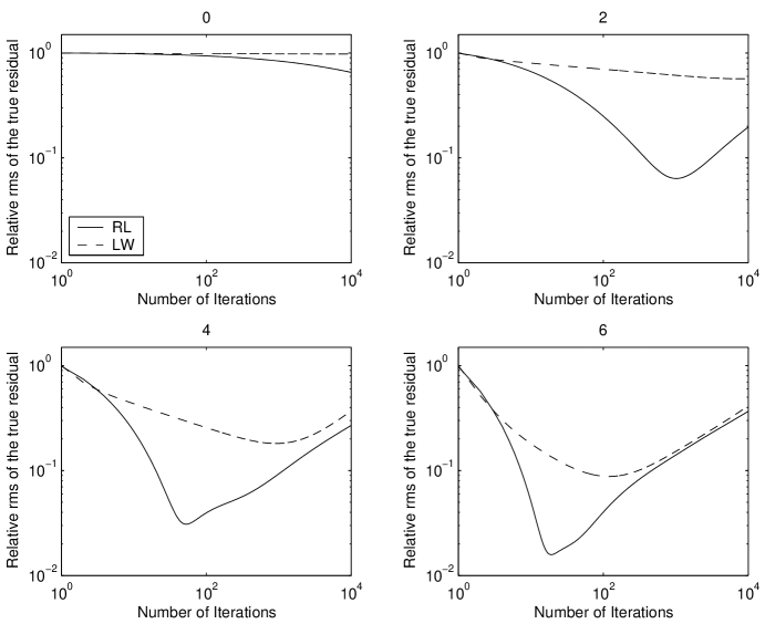
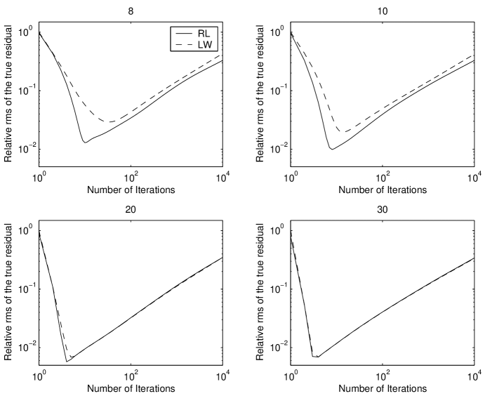
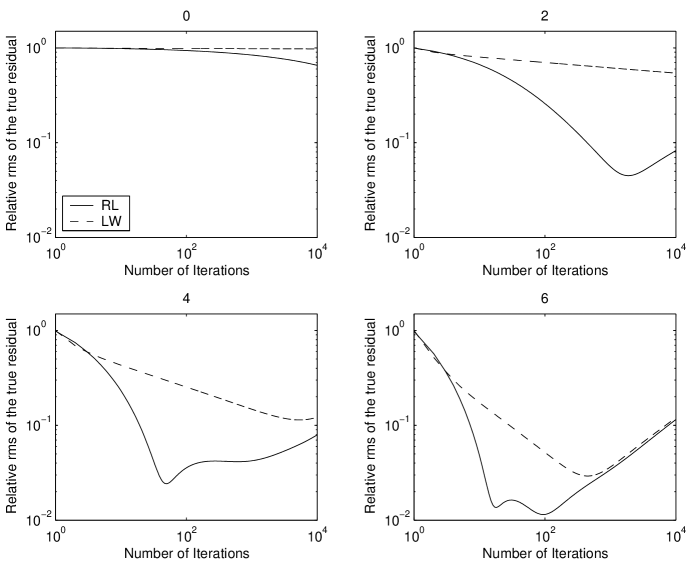
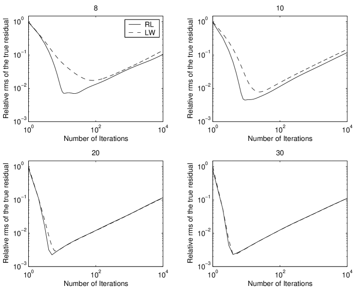
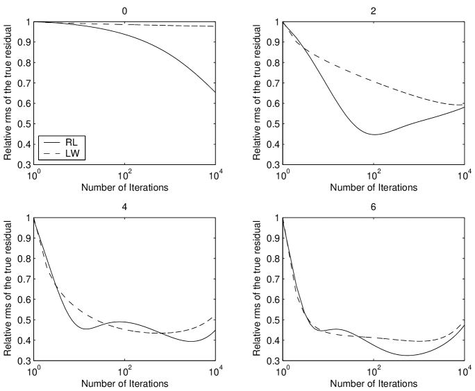
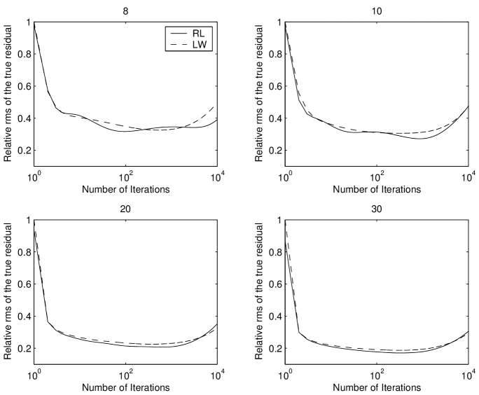
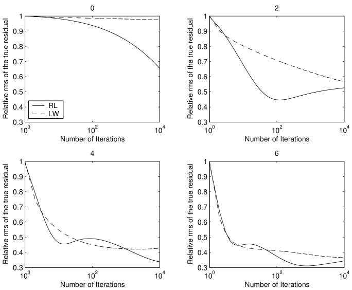
Since RL exploits the a priori knowledge regarding the statistics of photon counts, it should be expected to yield more accurate reconstructions than an approach that does not use this information. In reality, as shown by Figs. 20-27, the situation is not so clear. These figures provide the convergence rates and the performances of RL and LW methods for objects with a size that is increasing with respect to the size of the PSF (a two-dimensional Gaussian with circular symmetry). Two different types of objects are considered: a two-dimensional Gaussian and a rectangular function. Since the first target object presents an almost band-limited spectrum, whereas for the second target object the high-frequency Fourier components are important, their restorations represent very different problems. For both experiments, a background with an intensity of $1\%$ of the maximum value in the blurred image has been added. Finally, two different levels of noise have been considered corresponding to a peak ${\rm S/N}$ of $30$ and $40$ dB, respectively. The first case provides a background with an expected number of counts approximately equal to $30$, i.e., a level for which the Gaussian approximation of the Poissonian distribution is not very good.

From Figs. 20-27 it appears that the performance of RL for objects narrower than the PSF is, in general superior to LW for the band-limited target. The same is not true for the other objects. Interestingly, though, for extended objects, i.e. smooth objects with high intensity profiles over large regions, the performance of RL is roughly equivalent to that of LS (to properly compare the convergence rate, it is necessary to keep into account that, for each iteration, RL requires the computation of twice the number of two-dimensional DFT than is required by LW). This is especially true for the images characterized by the best ${\rm S/N}$. Motivated by these numerical results, we seek answers to the following questions: (i) why does RL perform better than LS on star-like objects, and (ii) why do the RL and LS approaches yield roughly the same results on extended objects?

4.1 RL vs LS: preliminary comments

It is important to note that in practice, when either the RL or LS approaches are used in solving image reconstruction problems, the exact computation of the maximum likelihood estimate (MLE) is not sought. For example, as was stated above, the LW iteration implements regularization via the iteration count. In fact, the objective when using LW is to stop the iteration late enough so that an accurate reconstruction is obtained, but before the reconstruction is corrupted by the noise in the high frequency components of the image. Notice, for example, that in Figs. 20-27 the relative error begins to increase at a certain point in both the RL and LW iterations.

As was stated above, one can show that the LW iterates are regularized solutions of $\boldsymbol{A}^{T}\boldsymbol{A}\boldsymbol{x}=\boldsymbol{A}^{T}\boldsymbol{b}$ via the singular value decomposition (SVD) of the matrix $\boldsymbol{A}$. Unfortunately, such an analysis of RL is impossible due to the nonlinearity in the RL algorithm. In particular, note the Hadamard multiplication and division in algorithm (17). Instead, we first note that if $\boldsymbol{A}$ is an invertible matrix, RL iterates converge to the MLE corresponding to the statistical model  (5) (see Wu 1983). Hence, RL can be viewed as an EM algorithm (Carasso 1999). The MLE is also the minimizer of the negative log-likelihood function associated with Eq. (5); namely,

$$J(\boldsymbol{x})=\boldsymbol{1}^{T}\left[\boldsymbol{A}\boldsymbol{x}-\boldsymbol{b}\odot\log(\boldsymbol{A}\boldsymbol{x})\right].$$ (25)

When the RL algorithm is used on image deblurring problems it exhibits a similar convergence behavior to that of the LW iteration. Specifically, for ill-conditioned problems, the RL iterates $\{\boldsymbol{x}_{k}\}$ provide more accurate reconstructions in early iterations (semiconvergence property), while in later iterations blow-up occurs (Lucy 1974; Carasso 1999). To explain why this occurs, we note that the function $\boldsymbol{J}$ is convex. In fact, assuming $A$ is positive definite, $\boldsymbol{J}$ is strictly convex. In this case, the minimum of $\boldsymbol{J}$ is the unique solution of the equation $\boldsymbol{\nabla}\boldsymbol{J}(\boldsymbol{x})=\boldsymbol{0}$, where $\boldsymbol{\nabla}\boldsymbol{J}$ is the gradient $\boldsymbol{J}$; that is,

$$\boldsymbol{A}^{T}\left(\boldsymbol{1}-\frac{\boldsymbol{b}}{\boldsymbol{A}\boldsymbol{x}}\right)=\boldsymbol{0}.$$ (26)

It is clear that provided $\boldsymbol{A}$ is invertible, the solution of (26) is obtained when $\boldsymbol{A}\boldsymbol{x}=\boldsymbol{b}$. That is, $\boldsymbol{x}_{*}=\boldsymbol{A}^{-1}\boldsymbol{b}$ is the solution of Eq. (26). Under the same conditions on $\boldsymbol{A}$, the LW iteration converges to the same value. Thus, we would expect that since blow-up occurs as $\boldsymbol{x}_{k}\rightarrow\boldsymbol{x}_{*}$ in the LW iteration when $\boldsymbol{A}$ is a poorly conditioned matrix, we will see the same results when we use RL. One consequence of this fact is that during reconstruction, RL uses, effectively, only a few frequencies and therefore cannot fully exploit prior statistical information regarding the noise (this should require the use of the entire spectrum).

4.2 RL vs. LS: a sensitivity analysis

In order to obtain a deeper understanding of the RL and LS approaches and to answer the two questions posed above, it is useful to introduce the quantities

$$\boldsymbol{\Delta}_{{\rm LW}}(\boldsymbol{x}_{k}) =-\boldsymbol{A}^{T}\boldsymbol{r}_{k};$$ (27)

$$\boldsymbol{\Delta}_{{\rm RL}}(\boldsymbol{x}_{k}) =-\boldsymbol{x}_{k}\odot\boldsymbol{A}^{T}\frac{\boldsymbol{r}_{k}}{\boldsymbol{A}\boldsymbol{x}_{k}},$$ (28)

which provide the correction to the solution $\boldsymbol{x}_{k}$ at the k-th iteration for LW and RL, respectively. Here,

$$\boldsymbol{r}_{k}=\boldsymbol{A}\boldsymbol{x}_{k}-\boldsymbol{b},$$ (29)

and, without loss of generality, we have set $\omega=1$ in the LW iteration. We note that in order to obtain Eq. (28) we needed the identity $\boldsymbol{A}^{T}\boldsymbol{1}=\boldsymbol{1}$ to hold. From these equations it is evident that at each iteration LW corrects the solution $\boldsymbol{x}_{k}$ with a quantity proportional to $\boldsymbol{r}_{k}$, while the correction provided by RL is proportional to $\boldsymbol{x}_{k}$ itself. Thus it is not surprising that RL outperforms LW when applied to reconstructing objects composed of star-like sources on a flat back ground, since in the early stages of both iterations the entries of $\boldsymbol{x}_{k}$ are large and increasing in regions corresponding to the positions of the objects in the image, while the values of $\boldsymbol{r}_{k}$ are correspondingly small and decreasing.

However, as has been shown by the simulations presented above, RL does not outperform LW when applied to reconstructing objects with smooth light distribution and whose spatial extension is broader than the PSF. In order to understand this phenomena, it is useful consider the negative Jacobian matrices of the quantities (27) and (28):

$$J_{LW}(\boldsymbol{x}_{k})=\boldsymbol{A}^{T}\boldsymbol{A}$$ (30)

and

$$J_{RL}(\boldsymbol{x}_{k}) =\hbox{diag}\left[\boldsymbol{A}^{T}\frac{\boldsymbol{r}_{k}}{\boldsymbol{A}\boldsymbol{x}_{k}}\right]$$

$$+\hbox{diag}[\boldsymbol{x}_{k}]\leavevmode\nobreak\ \boldsymbol{A}^{T}\hbox{diag}\left[\frac{\boldsymbol{b}}{\boldsymbol{A}\boldsymbol{x}_{k}\odot\boldsymbol{A}\boldsymbol{x}_{k}}\right]\boldsymbol{A}.$$ (31)

These matrices provide the sensitivities of the LW and RL algorithms to changes in the components of the iterate $\boldsymbol{x}_{k}$. Equations (30) and (4.2) allow us to make several observations. We begin by considering (30). Since in general astronomical applications $\boldsymbol{A}$ is the discretization of a PSF with an almost limited spatial support, the LW sensitivity matrix $\boldsymbol{A}^{T}\boldsymbol{A}$ will also have spatial support that is almost limited. From this observation, we can conclude that for a given pixel the corresponding component of the vector $\boldsymbol{\Delta}_{\rm LW}$ will be most sensitive to changes in the value of the pixel itself and in the values of “nearby” pixels. Here, the term “nearby” is defined by the characteristics of the PSF. More specifically, as the spread of the PSF increases, so does the collection of “nearby” pixels.

Perhaps an even more important observation, is that the sensitivity of the LW iteration to perturbations in $\boldsymbol{x}_{k}$ is independent of both $\boldsymbol{x}_{k}$ and $\boldsymbol{b}$. Consequently, the algorithm has no means of distinguishing between low and high intensity regions within the object, and hence, perturbations of the same magnitude are allowed for components of $\boldsymbol{x}_{k}$ corresponding to regions of both low and high light intensity. This explains why in areas of low light intensity (where the margin of error is very small) LW, and the least squares approach in general, does poorly.

The sensitivity matrix (4.2) for the RL iteration is more difficult to analyze. However, some simplification is possible when one considers the problem of the restoration of a flat background or of regions of an image in which the intensity distribution varies smoothly (e.g., the interior of the rectangular function considered in the simulations). In fact, in this case it is possible to define a region $\Omega$ where the image can be considered constant or almost constant. Because of the semiconvergence property of RL, in such regions the components of the vector $\boldsymbol{r}_{k}$ converge rapidly to zero (this has been verified via numerical simulations). Thus the first term in (4.2) converges to zero. The same is not true for the second term. Thus, it is reasonable to expect that it will provide an accurate approximation of the sensitivity of RL within $\Omega$.

Provided that the spread of the PSF is small relative to the size of $\Omega$, early in RL iterations the vector $\boldsymbol{x}_{k}$ is approximately constant and close to $\boldsymbol{b}$, i.e. those pixels values are reconstructed rapidly, within $\Omega$. Hence, the vector $\boldsymbol{b}/(\boldsymbol{A}\boldsymbol{x}_{k}\odot\boldsymbol{A}\boldsymbol{x}_{k})\approx 1/\boldsymbol{A}\boldsymbol{x}_{k}$ is also approximately constant within $\Omega$. In addition, if we define $\boldsymbol{D}_{\Omega}$ to be the diagonal matrix with components

$$[\boldsymbol{D}_{\Omega}]_{jj}=\left\{\begin{array}[]{ll}1,&j\in\Omega\\ 0,&j\notin\Omega\end{array}\right.,$$ (32)

then

$$\boldsymbol{D}_{\Omega}\boldsymbol{A}\boldsymbol{x}_{k}\approx\boldsymbol{D}_{\Omega}\boldsymbol{A}\boldsymbol{D}_{\Omega}\boldsymbol{x}_{k}$$ (33)

will be accurate within the interior of $\Omega$. To obtain (33) we used the fact that $\boldsymbol{x}_{k}$ is approximately constant on $\Omega$ and that the spread of $\boldsymbol{A}$ is small compared to the size of $\Omega$. Finally, the second term of (4.2) can be approximated within $\Omega$ as follows:

$$\boldsymbol{D}_{\Omega} \hbox{diag}[\boldsymbol{x}_{k}]\boldsymbol{A}^{T}\hbox{diag}[\boldsymbol{b}/(\boldsymbol{A}\boldsymbol{x}_{k}\odot\boldsymbol{A}\boldsymbol{x}_{k})]\boldsymbol{A}$$

$$\approx\hbox{diag}[\boldsymbol{x}_{k}]\boldsymbol{D}_{\Omega}\boldsymbol{A}^{T}\boldsymbol{D}_{\Omega}\hbox{diag}[\boldsymbol{b}/(\boldsymbol{A}\boldsymbol{x}_{k}\odot\boldsymbol{A}\boldsymbol{x}_{k})]\boldsymbol{A}$$ (34)

$$\approx\hbox{diag}[\boldsymbol{D}_{\Omega}(\boldsymbol{x}_{k}/\boldsymbol{A}\boldsymbol{x}_{k})]\boldsymbol{A}^{T}\boldsymbol{A}$$ (35)

$$\approx\boldsymbol{D}_{\Omega}\boldsymbol{A}^{T}\boldsymbol{A}.$$ (36)

Approximation (34) follows from (33). Approximation (35) follows from the fact that, as stated above, early in RL iterations $\boldsymbol{b}/(\boldsymbol{A}\boldsymbol{x}_{k}\odot\boldsymbol{A}\boldsymbol{x}_{k})\approx 1/\boldsymbol{A}\boldsymbol{x}_{k}$ is approximately constant. Thus we see that not only does the second term in (4.2) not converge to zero, it is well-approximated within $\Omega$ by the LW sensitivity (30). Recalling that the first term in (4.2) converges rapidly to zero in RL iterations, it is therefore not surprising that RL and LW provide similar results in the interior of the rectangular object mentioned above. We can extend this discussion to extended objects in general by noting that such objects can be decomposed into a union of regions in which the light intensity is approximately constant. Hence, RL and LW should provide similar results for extended objects in general.

4.3 RL vs. LS: convergence properties

As shown above, LW presents an acceptable convergence rate only in case of restoration of extended objects. Unfortunately, understanding the convergence properties of the RL algorithm (17) is a very difficult affair since it is not possible to carry out an analysis similar to that done in Sect. 3.2. For this reason, in order to obtain some insight, we consider, again, a noise-free signal $\boldsymbol{b}$ and Gaussian PSF with circular symmetry and variance $\sigma^{2}_{p}$. In addition, we suppose that the object of interest is a circular Gaussian source with variance $\sigma^{2}_{b}$. The amplitude of the source is not considered since RL conserves the total number of counts. Due to the connection between the RL and LW iterations discussed in the previous section, an understanding of RL convergence may provide further understanding of the convergence of the LW iteration. For simplicity, in what follows we work in the continuous, and results will be later discretized.

If a Gaussian function with variance $\sigma^{2}$ is denoted by $G[\sigma^{2}]$, the following facts are useful:

$$\frac{G[\sigma^{2}_{1}]}{G[\sigma^{2}_{2}]} =G\left[\frac{\sigma^{2}_{1}\sigma^{2}_{2}}{\sigma^{2}_{2}-\sigma^{2}_{1}}\right];$$ (37)

$$G[\sigma^{2}_{1}]\odot G[\sigma^{2}_{2}] =G\left[\frac{\sigma^{2}_{1}\sigma^{2}_{2}}{\sigma^{2}_{2}+\sigma^{2}_{1}}\right];$$ (38)

$$G[\sigma^{2}_{1}]\otimes G[\sigma^{2}_{2}] =G\left[\sigma^{2}_{1}+\sigma^{2}_{2}\right].$$ (39)

Here, the symbol “$\leavevmode\nobreak\ \otimes$” indicates convolution. From these equations it is evident that the result of any of the above operations produces a new Gaussian function. Only the first operation requires a condition be satisfied, i.e., $\sigma^{2}_{2}>\sigma^{2}_{1}$. This will always be satisfied during the RL iteration (see Eq. (42) below).

A point worth noting is that if we define $\sigma^{2}$ to be the variance of the Gaussians on the right hand side of (37)-(39), then for equation (37) we have $\sigma^{2}_{1}<\sigma^{2}$; in equation (38) we have $\sigma^{2}<\sigma^{2}_{1}<\sigma^{2}_{2}$; and in equation (39) we have $\sigma^{2}=\sigma^{2}_{1}+\sigma^{2}_{2}$. Consequently, only the operation (38) results in a Gaussian function with a variance that is smaller than both $\sigma_{1}$ and $\sigma_{2}$.

If the true object $\boldsymbol{x}$ is a Gaussian with variance $\sigma^{2}_{o}$, then using (39) and the fact that $\boldsymbol{A}\boldsymbol{x}=\boldsymbol{b}$, it is

$$\sigma^{2}_{b}=\sigma^{2}_{o}+\sigma^{2}_{p}.$$ (40)

As an initial guess in the RL algorithm, we take $\boldsymbol{x}_{0}=\boldsymbol{1}$.

Now, let’s suppose that $\boldsymbol{x}_{k}=G[\sigma^{2}_{k}]$. Using Eqs.  (37) - (39) one can obtain

$$G[\sigma^{2}_{k+1}]=G\left[\frac{\sigma^{2}_{k}(\sigma^{2}_{k}\sigma^{2}_{b}+\sigma^{4}_{p}+\sigma^{2}_{k}\sigma^{2}_{p})}{(\sigma^{2}_{k}+\sigma^{2}_{p})^{2}}\right].$$ (41)

It is a straightforward exercise to show that

$$R(\sigma^{2}_{k})=\frac{\sigma^{2}_{k+1}}{\sigma^{2}_{k}}=\frac{\sigma^{2}_{k}\sigma^{2}_{b}+\sigma^{4}_{p}+\sigma^{2}_{k}\sigma^{2}_{p}}{(\sigma^{2}_{k}+\sigma^{2}_{p})^{2}}<1$$ (42)

provided

$$\sigma^{2}_{k}>\sigma^{2}_{b}-\sigma^{2}_{p}.$$ (43)

To prove that (43) holds for all $k$, we use induction. First, note that since $\boldsymbol{x}_{0}=\boldsymbol{1}$, $\boldsymbol{A}^{T}\boldsymbol{1}=\boldsymbol{1}$, and $\boldsymbol{A}^{T}=\boldsymbol{A}$, we have that $\boldsymbol{x}_{1}=\boldsymbol{A}^{T}\boldsymbol{b}=G[\sigma_{p}^{2}+\sigma_{b}^{2}]$. Then $\sigma_{1}^{2}=\sigma_{p}^{2}+\sigma_{b}^{2}$, and hence, Eq. (43) is satisfied for $k=1$. Now, we show that if Eq. (43) holds for $k$, it must hold also for $k+1$. By replacing $\sigma_{k+1}^{2}$ in Eq. (43) by the argument of the Gaussian function on the right hand side of Eq. (41), one can obtain an equivalent inequality involving $\sigma_{k}^{2}$ given by

$$q(\sigma_{k}^{2})>0,$$ (44)

where $q(\sigma^{2})$ defined by

$$q(\sigma^{2}) = \sigma^{2}(\sigma^{2}\sigma^{2}_{b}+\sigma^{4}_{p}+\sigma^{2}\sigma^{2}_{p})+(\sigma_{p}^{2}-\sigma_{b}^{2})(\sigma^{2}+\sigma^{2}_{p})^{2}$$

$$= 2\sigma_{p}^{2}(\sigma^{2})^{2}+(3\sigma_{p}^{4}-2\sigma_{p}^{2}\sigma_{b}^{2})\sigma^{2}+(\sigma_{p}^{6}-\sigma_{b}^{2}\sigma_{p}^{4}).$$

Notice that $q$ is a quadratic function. We can therefore find its zeros via the quadratic formula. These are given by

$$\sigma^{2}=-\frac{\sigma_{p}^{2}}{2},\;\sigma_{b}^{2}-\sigma_{p}^{2}.$$ (45)

Since $\sigma_{p}^{2}>0$, we know that the graph of $q$ is an upward opening parabola. Furthermore, by (40) we have $\sigma_{b}^{2}-\sigma_{p}^{2}=\sigma_{o}^{2}>0$, and hence, we know that if $\sigma^{2}>\sigma_{b}^{2}-\sigma_{p}^{2}$, then $q(\sigma^{2})>0$. Thus (44) follows from the inductive hypothesis, and our proof is complete.

In light of these findings, it is possible to consider some convergence properties of the RL algorithm. We begin by showing that the sequence $\{\sigma_{k}^{2}\}$ converges to $\sigma_{o}^{2}=\sigma_{b}^{2}-\sigma_{p}^{2}$. First, note that Eqs. (42) and (43) imply that $\{\sigma_{k}^{2}\}$ is a decreasing sequence that is bounded below by $\sigma_{b}^{2}-\sigma_{p}^{2}$. Hence, $\{\sigma_{k}^{2}\}$ converges to some $\sigma^{*}\geq\sigma_{b}^{2}-\sigma_{p}^{2}$. From inequalities (42) and (43), we have that $R(\sigma_{*}^{2})=1$. Furthermore, the arguments used in the proof of (43) imply that if $\sigma^{2}>\sigma_{b}^{2}-\sigma_{p}^{2}$ then $R(\sigma^{2})<1$. Thus it must be that $\sigma_{*}^{2}=\sigma_{b}^{2}-\sigma_{p}^{2}$.

In regard to the convergence rate of the RL algorithm, Eq. (42) shows that, almost independently from the characterists of the object, in the very first iteration, when $\sigma_{b}\gg\sigma_{p}$, we have

$$R(\sigma^{2}_{0})=\frac{\sigma_{0}^{2}(\sigma_{b}^{2}+\sigma_{p}^{2})}{\sigma_{0}^{4}}\approx 0.$$ (46)

In fact, if $\boldsymbol{x}_{\boldsymbol{0}}=\boldsymbol{1}$ (i.e., $\sigma_{0}^{2}=\infty$), it is not difficult to see that $\boldsymbol{x}_{1}=\boldsymbol{A}\boldsymbol{b}$, i.e., the result of the first iteration is given by $G(\sigma_{p}^{2}+\sigma_{b}^{2})$. At this point, there are two possible situations:

1. For extended objects, we have $\sigma^{2}_{b}\approx\sigma^{2}_{1}\gg\sigma^{2}_{p}$. In this case, $R(\sigma^{2}_{1})\approx 1$. In general, this means that we can expect rapid progress in early iterations; after that the convergence rate slows down remarkably. This behavior is similar to that of the LW algorithm;

2. For stellar-like objects, we have $\sigma^{2}_{b}\approx\sigma^{2}_{p}$. Now, if we set $\sigma_{k}=\alpha\leavevmode\nobreak\ \sigma_{p}$, then

   $$R(\sigma^{2}_{k})=\frac{1+2\alpha^{2}}{(1+\alpha^{2})^{2}}.$$ (47)

   For example, when $\alpha=1,0.5,1/3,1/6$, then $R(\sigma^{2}_{k})=0.750,0.960,0.990,0.999$, respectively. In other words, although the convergence rate of RL slows down as the iteration progresses, this effect is not as pronounced as it is for the LW algorithm.

These statements are confirmed by Figs. 28, 29.

A comparison between the RL solution for star-like sources at the k-th iterate

$$\widehat{x}_{k}(i,j)\propto\exp{(-r^{2}/2\widehat{\sigma}_{k}^{2})}$$ (48)

with the corresponding LW solution

$$\widehat{x}_{k}(i,j)=\Pi_{k}(i,j),$$ (49)

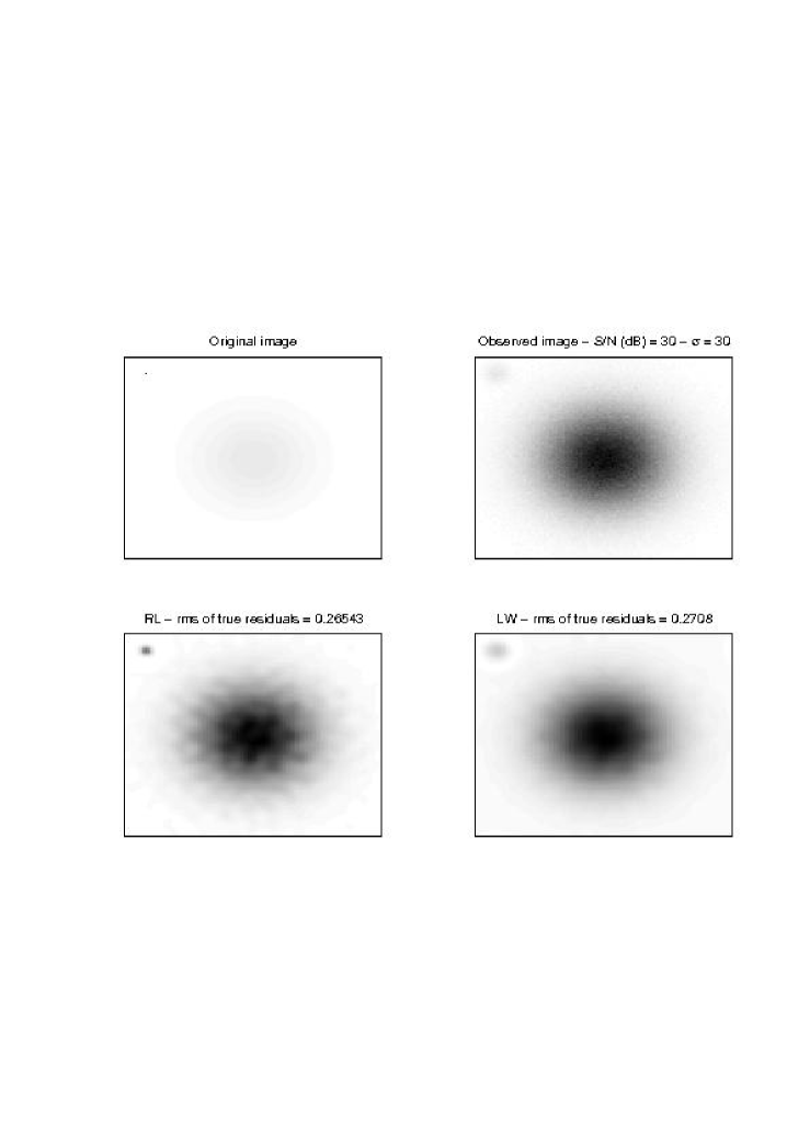
provides some additional insight into the convergence properties of these algorithms. In fact, from Eq. (48) it is evident that although the high frequencies are filtered in the RL algorithm, the filter is less stringent for high frequencies than is the Landweber filter. The consequence is that, in general, at a given $k$, RL has available a broader range of frequencies to restore the object. On the one hand, this can improve the convergence rate of RL compared to LW; on the other hand this could create problems when one or more star-like objects are superimposed with an extended object. In fact, a few RL iterations are sufficient to restore the extended object. The same is not true for the star-like objects. Therefore, more iterations are necessary. However, because of the amplification of the noise, this means the degradation of the results in the parts of the image not occupied by the star-like objects.

This effect is clearly visible in the experiment shown in Fig. 30.

5 Conclusions

In this paper we provide explanations for why, in spite the incorporation of a priori information regarding the noise statistics of image formation, the RL deblurring algorithm often does not provide results that are superior to those obtained by techniques based on an LS approach. In particular, we have identified a possible explanation in the regularization approaches of the specific algorithms. In fact, the adoption of a priori smoothness constraint in the Tikhonov approach, or the need to stop the iterations before blow-up occurs in the iterative approaches, e.g. both LW and RL, do not permit the full exploitation of the information contained in the highest Fourier frequencies, i.e., those where the specific nature of the noise has the largest influence. This has two consequences: I) the performance of the LS algorithms is almost insensitive to whether noise is Gaussian or Poissonian; II) the RL algorithm does not fully benefit from the fact that it incorporates the specific statistical model of the noise. In other words, the regularization of the solution implies a levelling out of the possible performances. In this respect, much more than a detailed knowledge of the nature of the noise is needed. Specifically, some rough a priori information regarding the solution, e.g. is it an extended or star-like object, is needed before one can know whether or not RL will provide superior results. Our numerical experiments support these conclusions. In particular, the fact that reconstructions gotten via the RL algorithm are often comparable to those of LW, i.e., an unsophisticated and very slow algorithm, indicates that resorting to advanced and often complex techniques is not always justified.

We stress that such conclusions are not only of academic interest. In fact, with respect to the ML algorithms, in general the LS algorithms are much easier to implement, are more flexible as concerns the incorporation of constraints, are more amenable to a theoretical analysis of their characteristics and are computationally less costly. Consequently, unless the use of a different approach is justified, they should be considered the standard approach.

Figure 1: Comparison of Poissonian vs. stationary Gaussian noise and corresponding power-spectra for the satellite image shown in Fig. 4. The variance of the two noises is the same.

Figure 2: Comparison of the results obtained by Tikhonov coupled with GCV in case of Poissonian and Gaussian noises (see text). The images have sizes $256\times 256$ pixels, the PSF is Gaussian with circular symmetry and dispersion set to $12$ pixels, ${\rm S/N}=20\leavevmode\nobreak\ {\rm dB}$. ${\rm rms}_{T}$ and ${\rm rms}_{I}$ are the rms of the true residuals calculated on the entire image and only on the pixels corresponding to the satellite, respectively.

Figure 3: Comparison of the results obtained by Tikhonov coupled with GCV in case of Poissonian and Gaussian noises (see text). The images have sizes $256\times 256$ pixels, the PSF is Gaussian with circular symmetry and dispersion set to $12$ pixels, ${\rm S/N}=30\leavevmode\nobreak\ {\rm dB}$. ${\rm rms}_{T}$ and ${\rm rms}_{I}$ are the rms of the true residuals calculated on the entire image and only on the pixels corresponding to the satellite, respectively.

Figure 4: Comparison of the results obtained by Tikhonov coupled with GCV in case of Poissonian and Gaussian noises (see text). The images have sizes $256\times 256$ pixels, the PSF is Gaussian with circular symmetry and dispersion set to $12$ pixels, ${\rm S/N}=40\leavevmode\nobreak\ {\rm dB}$. ${\rm rms}_{T}$ and ${\rm rms}_{I}$ are the rms of the true residuals calculated on the entire image and only on the pixels corresponding to the satellite, respectively.

Figure 5: Comparison of the results obtained by Tikhonov coupled with GCV in case of Poissonian and Gaussian noises (see text). The images have sizes $256\times 256$ pixels, the PSF is Gaussian with circular symmetry and dispersion set to $12$ pixels, ${\rm S/N}=60\leavevmode\nobreak\ {\rm dB}$. ${\rm rms}_{T}$ and ${\rm rms}_{I}$ are the rms of the true residuals calculated on the entire image and only on the pixels corresponding to the satellite, respectively.

Figure 6: Relationship between the estimates $\lambda_{g}$ and $\lambda_{p}$, corresponding to the Gaussian and the Poissonian noise, respectively, obtained in $100$ different realizations of the experiment shown in Fig. 3. The mean value and the standard deviation are $0.128$ and $4.55\times 10^{-4}$ for $\lambda_{g}$, and $0.128$ and $9.10\times 10^{-4}$ for $\lambda_{p}$.

Figure 7: Plot of $1-\widehat{\cal K}_{k}(r)$ vs. $r$ for different values of the iteration count $k$.

Figure 8: Comparison of the results obtained by Tikhonov coupled with GCV in case of Poissonian and Gaussian noises, This figures correspond to the experiment shown in Fig. 2. Panel $a)$ the coefficients $|\widehat{b}_{g}(i,j)|$ and $|\widehat{b}_{p}(i,j)|$ in decreasing order. The two horizontal lines represent the values of $\lambda$ for the two noises; b) corresponding GCV functions; c) coefficients $|\widehat{b}_{p}(i,j)|$ and $|\widehat{b}_{g}(i,j)|$ corresponding to the first $2000$ coefficients of $|\widehat{A}(i,j)|$ shown in panel a). The vertical lines show the indices of $|\widehat{b}(i,j)|$ closest to $\lambda$. d) $\Delta b(i,j)=|\widehat{b}_{g}(i,j)-\widehat{b}_{p}(i,j)|/|\widehat{b}_{g}(i,j)|$ vs. the corresponding first $2000$ coefficients of $|\widehat{A}(i,j)|$ with the largest modulus. ${\rm S/N}=20\leavevmode\nobreak\ {\rm dB}$.

Figure 9: Comparison of the results obtained by Tikhonov coupled with GCV in case of Poissonian and Gaussian noises, This figures correspond to the experiment shown in Fig. 3. Panel $a)$ the coefficients $|\widehat{b}_{g}(i,j)|$ and $|\widehat{b}_{p}(i,j)|$ in decreasing order. The two horizontal lines represent the values of $\lambda$ for the two noises; b) corresponding GCV functions; c) coefficients $|\widehat{b}_{p}(i,j)|$ and $|\widehat{b}_{g}(i,j)|$ corresponding to the first $2000$ coefficients of $|\widehat{A}(i,j)|$ shown in panel a). The vertical lines show the indices of $|\widehat{b}(i,j)|$ closest to $\lambda$. d) $\Delta b(i,j)=|\widehat{b}_{g}(i,j)-\widehat{b}_{p}(i,j)|/|\widehat{b}_{g}(i,j)|$ vs. the corresponding first $2000$ coefficients of $|\widehat{A}(i,j)|$ with the largest modulus. ${\rm S/N}=30\leavevmode\nobreak\ {\rm dB}$.

Figure 10: Comparison of the results obtained by Tikhonov coupled with GCV in case of Poissonian and Gaussian noises, This figures correspond to the experiment shown in Fig. 4. Panel $a)$ the coefficients $|\widehat{b}_{g}(i,j)|$ and $|\widehat{b}_{p}(i,j)|$ in decreasing order. The two horizontal lines represent the values of $\lambda$ for the two noises; b) corresponding GCV functions; c) coefficients $|\widehat{b}_{p}(i,j)|$ and $|\widehat{b}_{g}(i,j)|$ corresponding to the first $2000$ coefficients of $|\widehat{A}(i,j)|$ shown in panel a). The vertical lines show the indices of $|\widehat{b}(i,j)|$ closest to $\lambda$. d) $\Delta b(i,j)=|\widehat{b}_{g}(i,j)-\widehat{b}_{p}(i,j)|/|\widehat{b}_{g}(i,j)|$ vs. the corresponding first $2000$ coefficients of $|\widehat{A}(i,j)|$ with the largest modulus. ${\rm S/N}=40\leavevmode\nobreak\ {\rm dB}$.

Figure 11: Comparison of the results obtained by Tikhonov coupled with GCV in case of Poissonian and Gaussian noises, This figures correspond to the experiment shown in Fig. 5. Panel $a)$ the coefficients $|\widehat{b}_{g}(i,j)|$ and $|\widehat{b}_{p}(i,j)|$ in decreasing order. The two horizontal lines represent the values of $\lambda$ for the two noises; b) corresponding GCV functions; c) coefficients $|\widehat{b}_{p}(i,j)|$ and $|\widehat{b}_{g}(i,j)|$ corresponding to the first $2000$ coefficients of $|\widehat{A}(i,j)|$ shown in panel a). The vertical lines show the indices of $|\widehat{b}(i,j)|$ closest to $\lambda$. d) $\Delta b(i,j)=|\widehat{b}_{g}(i,j)-\widehat{b}_{p}(i,j)|/|\widehat{b}_{g}(i,j)|$ vs. the corresponding first $2000$ coefficients of $|\widehat{A}(i,j)|$ with the largest modulus. ${\rm S/N}=60\leavevmode\nobreak\ {\rm dB}$.

Figure 12: LW deblurring of the images shown in Fig. 2. ${\rm rms}_{T}$ and ${\rm rms}_{I}$ are the rms of the true residuals calculated on the entire image and only on the pixels corresponding to the satellite, respectively.

Figure 13: LW deblurring of the images shown in Fig. 3. ${\rm rms}_{T}$ and ${\rm rms}_{I}$ are the rms of the true residuals calculated on the entire image and only on the pixels corresponding to the satellite, respectively.

Figure 14: LW deblurring of the images shown in Fig. 4. ${\rm rms}_{T}$ and ${\rm rms}_{I}$ are the rms of the true residuals calculated on the entire image and only on the pixels corresponding to the satellite, respectively.

Figure 15: LW deblurring of the images shown in Fig. 5. ${\rm rms}_{T}$ and ${\rm rms}_{I}$ are the rms of the true residuals calculated on the entire image and only on the pixels corresponding to the satellite, respectively.

Figure 16: Convergence rate of the LW algorithm applied to the problem of deblurring the images shown in Fig. 2.

Figure 17: Convergence rate of the LW algorithm applied to the problem of deblurring the images shown in Fig. 3.

Figure 18: Convergence rate of the LW algorithm applied to the problem of deblurring the images shown in Fig. 4.

Figure 19: Convergence rate of the LW algorithm applied to the problem of deblurring the images shown in Fig. 5.

Figure 20: $\|\boldsymbol{x}_{k}-\boldsymbol{x}\|/\|\boldsymbol{x}\|$ vs. the number of iterations. The object of interest, located in the center of the image, is a two-dimensional Gaussian with circular symmetry and dispersion (in pixels) given in the top of each panel. It is superimposed to a background whose level is $1\%$ the peak value of the blurred image. The PSF is a two-dimensional Gaussian with a dispersion of $6$ pixels. The size of the image are $256\times 256$ pixels. The noise is Poissonian with peak ${\rm S/N}=30\leavevmode\nobreak\ {\rm dB}$. Two deblurring algorithms are used: Richardson-Lucy (RL) and LW.

Figure 21: As in Fig. 20.

Figure 22: As in Fig. 20 but with ${\rm S/N}=40\leavevmode\nobreak\ {\rm dB}$.

Figure 23: As in Fig. 20 but with ${\rm S/N}=40\leavevmode\nobreak\ {\rm dB}$.

Figure 24: $\|\boldsymbol{x}_{k}-\boldsymbol{x}\|/\|\boldsymbol{x}\|$ vs. the number of iterations. The object of interest, located in the center of the image, is of a two-dimensional rectangular function, with side length (in pixels) given in the top of each panel. It is superimposed to a background whose level is $1\%$ the peak value of the blurred image. The PSF is a two-dimensional Gaussian with a dispersion of $6$ pixels. The size of the image are $128\times 128$ pixels. The noise is Poissonian with peak ${\rm S/N}=30\leavevmode\nobreak\ {\rm dB}$. Two deblurring algorithms are used: Richardson-Lucy (RL) and LW.

Figure 25: As in Fig. 24.

Figure 26: As in Fig. 24 but with ${\rm S/N}=40\leavevmode\nobreak\ {\rm dB}$.

Figure 27: As in Fig. 24 but with ${\rm S/N}=40\leavevmode\nobreak\ {\rm dB}$.

Figure 28: $\sigma_{k}$ vs. the number of iterations for RL in the case of a Gaussian source with various values of $\sigma_{o}$ and a Gaussian PSF with dispersion $\sigma_{p}=6$.

Figure 29: $R^{1/2}(\sigma_{k}^{2})$ vs. the number of iterations for the cases shown in Fig. 28.

Figure 30: Deblurring results obtained with RL and LW for a star-like object superimposed with an extended source given by a Gaussian with circular symmetry and dispersion set to $30$ pixels. An additional background is present with a level set to $1\%$ the maximum of the noise-free blurred image. The PSF is a Gaussian with circular symmetry and dispersion set to $6$ pixels. The size of the image are $128\times 128$ pixels. The noise is Poissonian with peak ${\rm S/N}=30\leavevmode\nobreak\ {\rm dB}$. The image presented corresponds to the result with the smallest rms of the true residuals.

References

- Carasso (1999) Carasso, A.S. 1999, SIAM J. Numer. Anal., 36, 1659
- Feller (1971) Feller, W. 1971, An Introduction to Probability Theory and Its Applications, (Wiley, Philadelphia)
- Hansen (1997) Hansen, P.C. 1997, Rank-Deficient and Discrete Ill-Posed Problems (SIAM, Philadelphia)
- Johnson (1987) Johnson, M.E. 1987, Multivariate Statistical Simulation, (John Wiley & Sons, New York)
- Lucy (1974) Lucy, M. 1974, AJ, 79, 745
- Neelamani et al. (2004) Neelamani, R., Hyeokho, C., & Baraniuk, R. 2004, IEEE Transaction on Signal Processing, 52, 418
- Richardson (1972) Richardson, W. 1972, J. Opt. Soc. Am., 62, 55
- Shepp & Vardi (1982) Shepp, L., & Vardi, Y. 1984, IEEE Trans. Medical Imaging, 2, 113
- Snyder et. al (1993) Snyder, D.L., Hammoud, A.M., & White, R.L. 1993, JOSA A, 10, 1014
- Snyder et. al (1995) Snyder, D.L., Helstrom, C.W., Lanterman, Faisal, M., & White, R.L. 1995, JOSA A, 12, 272
- Starck et al, (2002) Starck, J.L, Pantin, E. & Murthag, F. 2002, PASP, 114, 1051
- Vio et al. (2003) Vio, R., Nagy, J., Tenorio, L., et al. 2003a, A&A, 401, 389
- Vogel (2002) Vogel, C. R. 2002, Computational Methods for Inverse Problems, (SIAM, Philadelphia)
- White (1991) White, R.L. 1991, in Proc. 1991 Conf. Inf. Sciences and Systems, 665, The Johns Hopkins University, Baltimore
- Wu (1983) Wu, C.F.J. 1983, The Anals of Statistics, 11, 95