Quantifying the uncertainties of chemical evolution studies

The stellar initial mass function and the stellar lifetimes are basic ingredients of chemical evolution models, for which different recipes can be found in the literature. In this paper, we quantify the effects on chemical evolution studies of the uncertainties in these two parameters. We concentrate on chemical evolution models for the Milky Way, because of the large number of good observational constraints. Such chemical evolution models have already ruled out significant temporal variations for the stellar initial mass function in our own Galaxy, with the exception perhaps of the very early phases of its evolution. Therefore, here we assume a Galactic initial mass function constant in time. Through an accurate comparison of model predictions for the Milky Way with carefully selected data sets, it is shown that specific prescriptions for the initial mass function in particular mass ranges should be rejected. As far as the stellar lifetimes are concerned, the major differences among existing prescriptions are found in the range of very low-mass stars. Because of this, the model predictions widely differ for those elements which are produced mostly by very long-lived objects, as for instance ³He and ⁷Li. However, it is concluded that model predictions of several important observed quantities, constraining the plausible Galactic formation scenarios, are fairly robust with respect to changes in both the stellar mass spectrum and the stellar lifetimes. For instance, the metallicity distribution of low-mass stars is nearly unaffected by these changes, since its shape is dictated mostly by the time scale for thin-disk formation.

1 Introduction

The formation and evolution of galaxies is one of the outstanding problems of astrophysics. In the last decade, a great deal of observational work has shed light on the production and distribution of chemical elements inside the Galaxy (e.g. Edvardsson et al. 1993; Cayrel 1996; Nissen & Schuster 1997; Gratton et al. 2000; Chen et al. 2003; Gratton et al. 2003; Ivans et al. 2003; Reddy et al. 2003; Zoccali et al. 2003; Akerman et al. 2004), often leading to an evolutionary scenario much more complicated than assumed in many models. Even more recently, abundance data have accumulated for external galaxies at both low and high redshift, thus providing precious information on the chemical evolution of different types of galaxies and on the early stages of galaxy evolution (e.g. Pettini 2001; Centurión et al. 2003; Dietrich et al. 2003a, b; Prochaska, Howk & Wolfe 2003; Tolstoy et al. 2003; Dessauges-Zavadsky et al. 2004; D’Odorico et al. 2004). In this framework, galactic chemical evolution models can be regarded as useful tools to discriminate among different scenarios of galaxy formation. In fact, as stressed many times in the literature, abundances and abundance ratios play a major rôle as cosmic clocks and give hints on the time scales of structure formation and evolution (Wheeler, Sneden & Truran 1989; Matteucci & François 1992; Matteucci 2001).

In order to build up a chemical evolution model, it is necessary to define the initial conditions and the basic physical laws governing the evolution of the system during the whole galactic lifetime. In short, one needs to specify whether the system is closed or open (should any inflow/outflow of gas occur), the chemical composition of the gas from which the computation starts and that of any infalling material, the stellar birthrate function and the stellar evolution and nucleosynthesis. In particular, the stellar birthrate is expressed as the product of two independent functions, the star formation rate (SFR) and the stellar initial mass function (IMF). The first is generally expressed as a function of time only, while the second, which describes the stellar mass distribution at birth, is likely to be universal (Kroupa 2002; but see e.g. Jeffries et al. 2004) and not vary as a function of time (Chiappini, Matteucci & Padoan 2000).

The free parameters that one introduces in the model simply reflect our poor understanding of the basic physical processes governing the formation and evolution of galactic structures. However, having a number of observational constraints formally larger than that of the free parameters allows us to restrict the range of variation of the parameters themselves and gain useful insight into the mechanisms of galaxy formation and evolution (Matteucci 2001). This is the case for our own Galaxy and will become soon the standard for an increasing number of external galaxies, thanks to the capabilities of modern telescopes and instrumentation.

In an epoch where the uncertainties in the data have become really small, it is worth trying to consider ‘theoretical error bars’ as well. An attempt to do so has recently been done by Romano et al. (2003), who compare the evolution of light elements predicted by two independent models of chemical evolution for the Milky Way and try to ascertain the origin of the differences in the model predictions. In the present paper we intend to assess the uncertainties in the model predictions which arise when exploring different prescriptions for the IMF and the stellar lifetimes in a model for the Milky Way. To this purpose, we adopt a chemical evolution model which has been proven to successfully reproduce the main observational features of the solar neighbourhood (Chiappini, Matteucci & Gratton 1997) and change the assumptions on the stellar IMF. As a result, we set up a range of possible variations for several predicted quantities. Then, we repeat the same kind of analysis by changing the prescriptions for the stellar lifetimes.

The paper is organized as follows. In Section 2, we review the general features of the IMF which have emerged over the years and emphasize differences and similarities among the various IMFs adopted in this work. In Section 3, we discuss the prescriptions for the stellar lifetimes. In Section 4, we describe the chemical evolution model for the solar vicinity. In Section 5 we present model results. Finally, Section 6 is devoted to a critical discussion of the problem and some conclusions are drawn. Notice that the paper is structured in such a way that it is easy to concentrate on only one among the proposed topics, while skipping the others, if one wishes to do so.

2 The stellar initial mass function

2.1 The adopted parametrizations

Table 1: ${\mathrm{I}}(m_{1},\,m_{2})$ (see text for a definition of this quantity) for different mass intervals for the various IMFs considered in this study.

$\mathrm{Mass\;range}$	${\mathrm{I}}(m_{1},\,m_{2})$
$(m_{1},\,m_{2})$	${\mathrm{Salpeter\;(1955)}}$	${\mathrm{Tinsley\;(1980)}}$	${\mathrm{Scalo\;(1986)}}$	${\mathrm{Kroupa\;et\;al.(1993)}}$	${\mathrm{Scalo\;(1998)}}$	${\mathrm{Chabrier\;(2003)}}$
$0.1$–$0.5$	$0.472814$	$0.340757$	$0.52945$	$0.343983$	$0.205694$	$0.246036$
$0.5$–$0.6$	$0.0386389$	$0.0386018$	$0.0432673$	$0.0637846$	$0.0446104$	$0.0404886$
$0.6$–$1.0$	$0.0960027$	$0.108154$	$0.107502$	$0.166806$	$0.165927$	$0.119639$
$1.0$–$2.0$	$0.105638$	$0.146756$	$0.118292$	$0.170327$	$0.217311$	$0.148891$
$2.0$–$5.0$	$0.105561$	$0.169621$	$0.10199$	$0.129128$	$0.164747$	$0.154816$
$5.0$–$8.0$	$0.0423486$	$0.0705069$	$0.0318011$	$0.0402628$	$0.0513691$	$0.0643529$
$8.0$–$40$	$0.102002$	$0.184335$	$0.0551705$	$0.0698502$	$0.108612$	$0.162753$
$40$–$100$	$0.0369948$	$0.00322992$	$0.0125267$	$0.0158598$	$0.0417308$	$0.0630242$

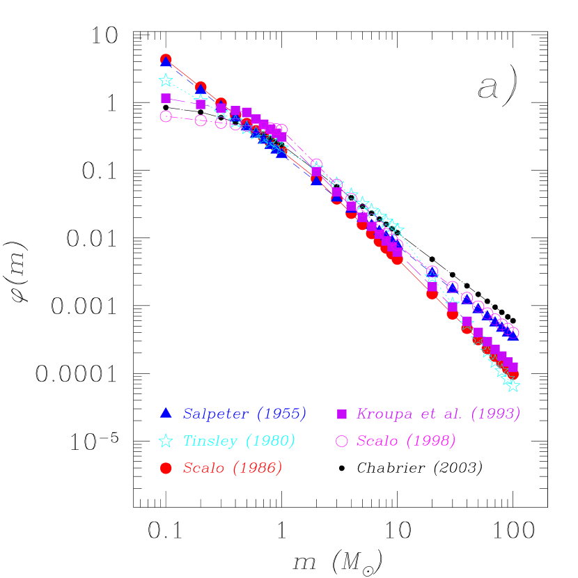
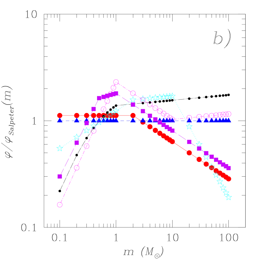
Figure 1: a) Stellar IMF according to Salpeter (1955; triangles), Tinsley (1980; stars), Scalo (1986; full circles), Kroupa et al. (1993; squares), Scalo (1998; empty circles) and Chabrier (2003; dots). Here $\varphi(m)$ is the IMF by mass and $\varphi(m)\propto m^{-x}$ ($x$ = 1.35 in the case of Salpeter’s IMF), except for Chabrier (2003), where a lognormal form for the low-mass domain ($m\leq$ 1 $M_{\odot}$) is suggested instead (see text). Here the Chabrier IMF also has $x$ = 1.3 as the exponent in the $m>$ 1 $M_{\odot}$ mass domain. b) Same as panel a), but with $\varphi(m)$ divided by the corresponding Salpeter value for each given mass. This allows a first sight comparison of the various mass distributions expected according to the different IMFs with respect to the ‘standard’ Salpeter choice.

The most widely used functional form for the IMF is an extension of that proposed by Salpeter (1955) to the whole stellar mass range:

$$\phi_{\mathrm{Salpeter}}(m)=\mathscr{A}_{\mathrm{Salpeter}}\,m^{-(1+x)},$$

where $x$ = 1.35 and

$$\int_{m_{\mathrm{low}}}^{m_{\mathrm{up}}}m\,\phi_{\mathrm{Salpeter}}(m){\mathrm{d}}m=1.$$

Here the IMF is by number; $m_{\mathrm{low}}$ = 0.1 $M_{\odot}$, $m_{\mathrm{up}}$ = 100 $M_{\odot}$ and $\mathscr{A}_{\mathrm{Salpeter}}\simeq$ 0.17. The above formula equivalently reads

$$\int_{m_{\mathrm{low}}}^{m_{\mathrm{up}}}\varphi_{\mathrm{Salpeter}}(m){\mathrm{d}}m=1$$

if using the IMF by mass, $\varphi_{\mathrm{Salpeter}}(m)\propto m^{-1.35}$. In what follows we always use the IMF by mass.

More realistic, multi-slope expressions better describe the luminosity function of main sequence stars in the solar neighbourhood, that is what is actually observed (Tinsley 1980; Scalo 1986; Kroupa, Tout & Gilmore 1993; Scalo 1998; see the original publications for details):

$$\varphi_{\mathrm{Tinsley}}(m)=\left\{\begin{array}[]{l l}\mathscr{A}_{\mathrm{Tinsley}}\,m^{-1.0}&\qquad{\mathrm{if}}\;m<2\,M_{\odot}\\ \mathscr{B}_{\mathrm{Tinsley}}\,m^{-1.3}&\qquad{\mathrm{if}}\;2<m/M_{\odot}<10\\ \mathscr{C}_{\mathrm{Tinsley}}\,m^{-2.3}&\qquad{\mathrm{if}}\;m>10\,M_{\odot},\\ \end{array}\right.$$

$$\mathscr{A}_{\mathrm{Tinsley}}\simeq 0.21,\;\mathscr{B}_{\mathrm{Tinsley}}\simeq 0.26,\;\mathscr{C}_{\mathrm{Tinsley}}\simeq 2.6;$$

$$\varphi_{\mathrm{Scalo\,86}}(m)=\left\{\begin{array}[]{l l}\mathscr{A}_{\mathrm{Scalo\,86}}\,m^{-1.35}&\qquad{\mathrm{if}}\;m<2\,M_{\odot}\\ \mathscr{B}_{\mathrm{Scalo\,86}}\,m^{-1.70}&\qquad{\mathrm{if}}\;m>2\,M_{\odot},\\ \end{array}\right.$$

$$\mathscr{A}_{\mathrm{Scalo\,86}}\simeq 0.19,\;\mathscr{B}_{\mathrm{Scalo\,86}}\simeq 0.24$$

(notice that we adopt a simplified two-slope approximation to the actual Scalo 1986 formula, similarly to what is done in Matteucci & François 1989);

$$\varphi_{\mathrm{Kroupa}}(m)=\left\{\begin{array}[]{l l}\mathscr{A}_{\mathrm{Kroupa}}\,m^{-0.3}&\qquad{\mathrm{if}}\;m<0.5\,M_{\odot}\\ \mathscr{B}_{\mathrm{Kroupa}}\,m^{-1.2}&\qquad{\mathrm{if}}\;0.5<m/M_{\odot}<1\\ \mathscr{C}_{\mathrm{Kroupa}}\,m^{-1.7}&\qquad{\mathrm{if}}\;m>1\,M_{\odot},\\ \end{array}\right.$$

$$\mathscr{A}_{\mathrm{Kroupa}}\simeq 0.58,\;\mathscr{B}_{\mathrm{Kroupa}}=\mathscr{C}_{\mathrm{Kroupa}}\simeq 0.31;$$

$$\varphi_{\mathrm{Scalo\,98}}(m)=\left\{\begin{array}[]{l l}\mathscr{A}_{\mathrm{Scalo\,98}}\,m^{-0.2}&\qquad{\mathrm{if}}\;m<1\,M_{\odot}\\ \mathscr{B}_{\mathrm{Scalo\,98}}\,m^{-1.7}&\qquad{\mathrm{if}}\;1<m/M_{\odot}<10\\ \mathscr{C}_{\mathrm{Scalo\,98}}\,m^{-1.3}&\qquad{\mathrm{if}}\;m>10\,M_{\odot},\\ \end{array}\right.$$

$\mathscr{A}_{\mathrm{Scalo\,98}}=\mathscr{B}_{\mathrm{Scalo\,98}}\simeq$ 0.39, $\mathscr{C}_{\mathrm{Scalo\,98}}\simeq$ 0.16. All of them are considered in the present work. The normalization is always performed in the mass range 0.1–100 $M_{\odot}$.

More recently, a lognormal form has been suggested for the low-mass part of the IMF ($m\leq$ 1 $M_{\odot}$), eventually extending into the substellar regime (Chabrier 2003):

$$\varphi_{\mathrm{Chabrier}}(m)=\left\{\begin{array}[]{l}\mathscr{A}_{\mathrm{Chabrier}}\,{\mathrm{e}}^{-(\log m-\log m_{\mathrm{c}})^{2}/2\,\sigma^{2}}\\ \qquad\qquad\qquad\qquad\qquad{\mathrm{if}}\;m\leq 1\,M_{\odot}\\ \mathscr{B}_{\mathrm{Chabrier}}\,m^{-(1.3\pm 0.3)}\\ \qquad\qquad\qquad\qquad\qquad{\mathrm{if}}\;m>1\,M_{\odot}.\\ \end{array}\right.$$

According to Chabrier (2003), the IMF depends weakly on the environment, except perhaps for early star formation conditions. Values of $m_{\mathrm{c}}$ = 0.079 $M_{\odot}$ and $\sigma$ = 0.69 well characterize the IMF for single objects belonging to the Milky Way disk. For $m>1$ $M_{\odot}$, we assume a power-law exponent $x$ equal to either 1.3 or 1.7. In the latter case, we study both an IMF truncated at $m_{\mathrm{low}}$ = 0.1 $M_{\odot}$ and one extending down to $m_{\mathrm{low}}$ = 0.001 $M_{\odot}$, i.e., into the brown dwarf (BD) domain. The normalization constants are: $\mathscr{A}_{\mathrm{Chabrier}}\simeq$ 0.85, $\mathscr{B}_{\mathrm{Chabrier}}\simeq$ 0.24 for $x$ = 1.3, $m_{\mathrm{low}}$ = 0.1 $M_{\odot}$; $\mathscr{A}_{\mathrm{Chabrier}}\simeq$ 1.16, $\mathscr{B}_{\mathrm{Chabrier}}\simeq$ 0.32 for $x$ = 1.7, $m_{\mathrm{low}}$ = 0.1 $M_{\odot}$; $\mathscr{A}_{\mathrm{Chabrier}}\simeq$ 1.06, $\mathscr{B}_{\mathrm{Chabrier}}\simeq$ 0.30 for $x$ = 1.7, $m_{\mathrm{low}}$ = 0.001 $M_{\odot}$.

Table 2: ${\mathrm{I}}(m_{1},\,m_{2})$ for different mass ranges in case of Chabrier (2003) IMF with $x$ = 1.7. The normalization is performed either in the mass range 0.1–100 $M_{\odot}$ (second column) or in the mass range 0.001–100 $M_{\odot}$ (third column).

$\mathrm{Mass\;range}$	${\mathrm{I}}(m_{1},\,m_{2})$
$(m_{1},\,m_{2})$	${\mathrm{Chabrier\;(2003);\;steeper,\;without\;BDs}}$	${\mathrm{Chabrier\;(2003);\;steeper,\;with\;BDs}}$
$0.001$–$0.1$	$-$	$0.0882928$
$0.1$–$0.5$	$0.335882$	$0.306225$
$0.5$–$0.6$	$0.0552738$	$0.0503936$
$0.6$–$1.0$	$0.163328$	$0.148907$
$1.0$–$2.0$	$0.178369$	$0.162621$
$2.0$–$5.0$	$0.135225$	$0.123286$
$5.0$–$8.0$	$0.0421639$	$0.0384412$
$8.0$–$40$	$0.0731485$	$0.0666901$
$40$–$100$	$0.0166087$	$0.0151423$

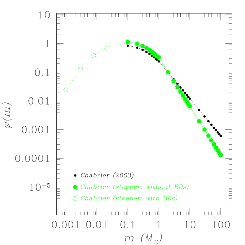
Figure 2: Stellar IMF according to Chabrier (2003). A power law is assumed for $m\geq$ 1 $M_{\odot}$, with an exponent $x$ = 1.3 (dots) or $x$ = 1.7 (pentagons). For $m<$ 1 $M_{\odot}$, a lognormal form is proposed, eventually extending into the BD domain (open pentagons).

The question of whether the IMF is universal or varies with varying star-forming conditions has been long debated in the past. Combining recent IMF estimates for different populations in which individual stars have been resolved unveils an extraordinary uniformity of the IMF (Kroupa 2002), although some room for exceptions is left (e.g., Aloisi, Tosi & Greggio 1999). Explaining the chemo-photometric properties of elliptical galaxies has often required an IMF biased towards massive stars (e.g. Arimoto & Yoshii 1987). However, the actual IMF slope cannot be inferred from direct observations in this case.

2.2 Differences and similarities among different parametrizations

In Fig. 1a we compare Salpeter (1955; triangles), Tinsley (1980; stars), Scalo (1986; full circles), Kroupa et al. (1993; squares), Scalo (1998; empty circles) and Chabrier (2003; dots) IMFs. For the Chabrier IMF the dots for $m\geq$ 1 $M_{\odot}$ display the power-law form with an exponent $x=$ 1.3. For all these IMFs, the normalization is performed in the mass range 0.1–100 $M_{\odot}$.

It is immediately seen that a Salpeter or a Scalo (1986) IMF predicts many more stars at the very low end of the distribution than a Scalo (1998) or a Chabrier IMF. Tinsley’s IMF lies somewhere in the middle, while it predicts the highest fraction of stars in the mass range 2–10 $M_{\odot}$. These features appear more clearly in Fig. 1b, where the IMFs are divided by the corresponding Salpeter value for each given mass.

In order to quantify the relative weights of stars belonging to different mass ranges according to different IMFs, we compute the following quantities:

$${\mathrm{I}}(m_{1},m_{2})=\int_{m_{1}}^{m_{2}}\varphi(m){\mathrm{d}}m,$$

for each of the IMFs discussed above. The results are listed in Table 1. The integration limits, $m_{1}$ and $m_{2}$, are properly chosen in order to allow a meaningful comparison when discussing the rôle played by stars belonging to different mass intervals in polluting the interstellar medium (ISM) with different chemical elements while varying the IMF prescriptions (Section 5.1).

In Fig. 2 we show the effect of steepening Chabrier (2003) IMF for $m\geq$ 1 $M_{\odot}$. A value of $x$ = 1.7 (pentagons) is now assumed instead of $x$ = 1.3 (dots). A steeper IMF for stars more massive than a few solar masses seems to be more likely, on the grounds of recent results by Kroupa & Weidner (2003). Those authors argue that field IMFs for early-type stars must be steeper than the Salpeter approximation, owing to the fact that a Salpeter power law well describes the distribution of stellar masses for local star formation events in star clusters. A steep field-star IMF thus arises naturally because of the power-law cluster mass function according to which star clusters distribute.

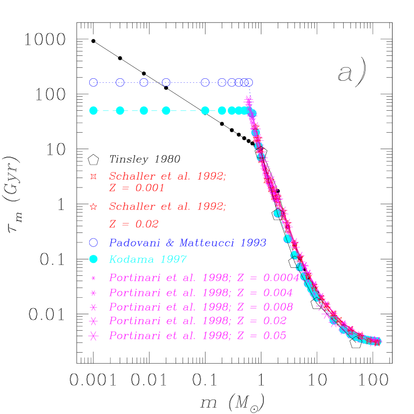
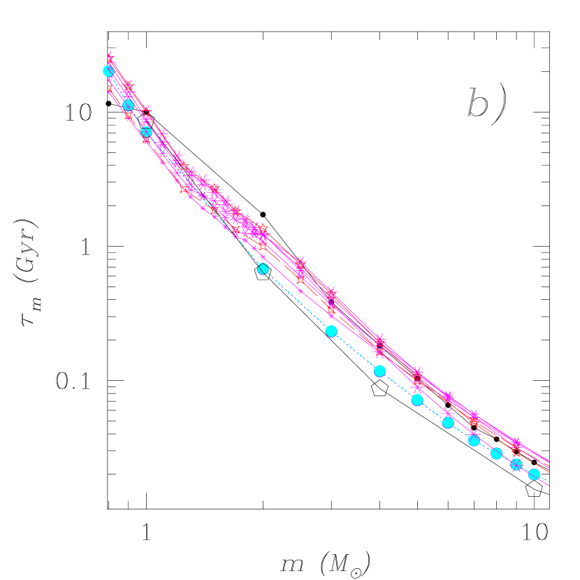
Figure 3: a) Stellar lifetimes as a function of the initial mass of the star: Maeder & Meynet (1989; dots); Tinsley (1980; pentagons); Schaller et al. (1992; stars); Padovani & Matteucci (1993; empty circles); Kodama (1997; filled circles); Portinari et al. (1998; asterisks). b) A zoom of the 1–10 $M_{\odot}$ stellar mass range.

Fig. 2 also shows the behaviour of Chabrier IMF for $m<$ 1 $M_{\odot}$. It is seen that the mass distribution flattens below $m\simeq$ 1 $M_{\odot}$, reaches a peak around $m\simeq$ 0.1 $M_{\odot}$ and then decreases smoothly for $m<$ 0.1 $M_{\odot}$. As a consequence, less than 10% of the stellar mass should be found in form of BDs (see also Table 2).

In Section 5.1 we illustrate the results obtained for the solar vicinity when the different parametrizations listed above are adopted.

3 The stellar lifetimes

Different authors traditionally adopt different prescriptions for the stellar lifetimes. For instance, Matteucci and coworkers have usually assumed stellar lifetimes from Maeder & Meynet (1989):

$$\tau_{m}=\left\{\begin{array}[]{l l}10^{-0.6545\log m+1}&\quad{\mathrm{for\;}}m\leq 1.3\;M_{\odot}\\ 10^{-3.7\log m+1.35}&\quad{\mathrm{for\;}}1.3<m/M_{\odot}\leq 3\\ 10^{-2.51\log m+0.77}&\quad{\mathrm{for\;}}3<m/M_{\odot}\leq 7\\ 10^{-1.78\log m+0.17}&\quad{\mathrm{for\;}}7<m/M_{\odot}\leq 15\\ 10^{-0.86\log m-0.94}&\quad{\mathrm{for\;}}15<m/M_{\odot}\leq 60\\ 1.2\,m^{-1.85}+0.003&\quad{\mathrm{for\;}}m>60\;M_{\odot},\\ \end{array}\right.$$

with $\tau_{m}$ in units of Gyr. Notice that they extrapolated the values for $m\leq$ 1.3 $M_{\odot}$ and $m>$ 60 $M_{\odot}$, since Maeder & Meynet (1989) do not give any formula for these mass ranges. The adopted extrapolation to larger masses is compatible with the values reported by Maeder & Meynet for stars of 85 and 120 $M_{\odot}$ (their table 2).

These stellar lifetimes differ widely from other formulations available in the literature, especially in the low-mass range ($m<$ 1 $M_{\odot}$). Tinsley (1980) and Tosi (1982 and subsequent papers) have:

$$\begin{array}[]{l l}\tau_{m}>8.6&\quad{\mathrm{for\;}}m<1\;M_{\odot}\\ 8.6>\tau_{m}>0.64&\quad{\mathrm{for\;}}1<m/M_{\odot}<2\\ 0.64>\tau_{m}>0.087&\quad{\mathrm{for\;}}2<m/M_{\odot}<4\\ 0.087>\tau_{m}>\sim 0.0155&\quad{\mathrm{for\;}}4<m/M_{\odot}<10\\ \sim 0.0155>\tau_{m}>\sim 0.003&\quad{\mathrm{for\;}}10<m/M_{\odot}<50\\ \end{array}$$

(see Tinsley 1980 for references).

Kodama (1997) reports:

$$\tau_{m}=\left\{\begin{array}[]{l}50\quad{\mathrm{for\;}}m\leq 0.56\;M_{\odot}\\ 10^{\big{(}0.334-\sqrt{1.790-0.2232\times(7.764-\log m)}\big{)}\big{/}0.1116}\\ \qquad\qquad\qquad\qquad\qquad\qquad\qquad{\mathrm{for\;}}m\leq 6.6\;M_{\odot}\\ 1.2\,m^{-1.85}+0.003\quad{\mathrm{for\;}}m>6.6\;M_{\odot},\\ \end{array}\right.$$

similarly to what suggested by Padovani & Matteucci (1993 and references therein):

$$\tau_{m}=\left\{\begin{array}[]{l}160\quad{\mathrm{for\;}}m\leq 0.60\;M_{\odot}\\ 10^{\big{(}0.334-\sqrt{1.790-0.2232\times(7.764-\log m)}\big{)}\big{/}0.1116}\\ \qquad\qquad\qquad\qquad\qquad\qquad\qquad{\mathrm{for\;}}m\leq 6.6\;M_{\odot}\\ 1.2\,m^{-1.85}+0.003\quad{\mathrm{for\;}}m>6.6\;M_{\odot}.\\ \end{array}\right.$$

It is seen that ancient very low-mass stars (0.6 $\leq m/M_{\odot}\leq$ 0.9) die in a Hubble time according to Matteucci & François (1989) extrapolation of Maeder & Meynet (1989) formulæ, whereas they have a longer life according to other authors. On the contrary, following Maeder & Meynet (1989) stars with 1 $<m/M_{\odot}<$ 2 live longer than in any other study.

In Fig. 3 we compare all the above-mentioned parametrizations, as well as values obtained from Geneva (Schaller et al. 1992) and Padua (Portinari et al. 1998 and references therein) stellar tracks. In the low- and very low-mass stellar mass domain substantial differences are found, while smaller, though not negligible, differences exist at higher masses. Detailed analyses of the results obtained when integrating these differences over the Galactic lifetime and IMF are reported in Section 5.2.

4 The chemical evolution model for the solar neighbourhood

In order to follow the chemical evolution of the solar vicinity, we adopt the two-infall model of Chiappini et al. (1997). According to this model, the halo and part of the thick-disk population form out of a first infall episode on a short time scale, while the thin disk accumulates much more slowly during a second independent infall episode. The rate of accretion of matter is

$$\frac{\mathrm{d}\Sigma_{\mathrm{inf}}(t)}{\mathrm{d}t}=A\,\mathrm{e}^{-t/\tau_{\mathrm{H}}}+B\,\mathrm{e}^{-(t-t_{\mathrm{max}})/\tau_{\mathrm{D}}},$$

where $\Sigma_{\mathrm{inf}}(t)$ is the mass surface density of the infalling primordial matter at time $t$. The parameters $t_{\mathrm{max}}$ = 1 Gyr, $\tau_{\mathrm{H}}$ = 0.8 Gyr and $\tau_{\mathrm{D}}$ = 7 Gyr are the time of maximum infall onto the disk and the time scales for mass accretion onto the halo/thick-disk and thin-disk components, respectively. They are fixed by the request of reproducing a number of observational constraints (Matteucci 2001). The coefficients $A$ and $B$ are derived from the condition of reproducing the current total mass surface density at the solar position (Chiosi 1980). Obviously, the coefficient $B$ must be zero for $t<t_{\mathrm{max}}$.

The SFR is

$$\psi(t)=\nu(t)\bigg{[}\frac{\Sigma(t_{\mathrm{Gal}})}{\Sigma(t)}\bigg{]}^{k-1}G^{k}(t),$$

proportional to both the total mass and gas surface densities. Here $G(t)$ is the normalized gas surface density, $\Sigma_{\mathrm{gas}}(t)/\Sigma(t_{\mathrm{Gal}})$, and $\Sigma(t_{\mathrm{Gal}})$ is the total mass surface density at the present time, $t_{\mathrm{Gal}}$ = 13.7 Gyr. A gas exponent $k$ = 1.5 guarantees a good agreement between model predictions and observations (Chiappini et al. 1997). Moreover, it is found to agree with inferences from observations (Kennicutt 1998) and $N$-body simulations (Gerritsen & Icke 1997).

The star formation efficiency, $\nu(t)$, is set to 2 Gyr^-1 during the halo/thick-disk phase and to 1.2 Gyr^-1 during the thin-disk phase to ensure the best fit to all the observed features of the solar vicinity, unless the gas surface density drops below a critical threshold, $\Sigma_{\mathrm{gas}}^{\mathrm{th}}\sim$ 7 $M_{\odot}$ pc^-2. In this case $\nu$ = 0 and the star formation ceases. This naturally explains the existence of a gap in the SFR between the halo/thick-disk and the thin-disk phase (Gratton et al. 1996, 2000; Fuhrmann 1998, 2004). Moreover, it delays the beginning of the star formation in the halo to the time at which the critical gas density can be reached.

The instantaneous recycling approximation is relaxed, i.e. the stellar lifetimes are taken into account in details. Stellar nucleosynthesis is taken from (i) van den Hoek & Groenewegen (1997) for low- and intermediate-mass stars (their case with metallicity-dependent mass loss efficiency along the asymptotic giant branch); (ii) Woosley & Weaver (1995) for massive stars; (iii) Thielemann, Nomoto & Hashimoto (1993) for Type Ia supernovae (SNeIa); (iv) José & Hernanz (1998) for classical novae. The carbon yields from massive stars in the mass range $m\geq$ 40 $M_{\odot}$ are multiplied by a factor of three (arguments are given in Chiappini, Romano & Matteucci 2003a). Stellar production and/or destruction of the light elements deuterium, ³He and ⁴He are included in the model according to Dearborn, Steigman & Tosi (1996), Galli et al. (1997) and Chiappini, Renda & Matteucci (2002) prescriptions. ⁷Li production/destruction is accounted for following Romano et al. (2001, 2003) and references therein.

The prescriptions on the IMF and the stellar lifetimes are changed according to the above discussions (Sections 2 and 3).

5 Quantifying the uncertainties in chemical evolution model predictions

5.1 Changing the IMF

In this section we discuss the results obtained by varying the prescriptions on the stellar IMF in the chemical evolution code for the solar vicinity. The purpose is to associate errors due to uncertainties in the stellar IMF to chemical evolution model results.

During the Galactic lifetime, many successive stellar generations form according to the adopted IMF (see e.g. Tables 1 and 2). As a result, for each IMF choice the composite stellar population, determining the global chemical properties of the Galaxy, is more or less enriched in stars falling in a given mass range. Hence the model predictions on specific quantities related to the given mass range vary when changing the IMF prescriptions.

As a first example, Fig. 4 displays the theoretical G-dwarf metallicity distribution predicted by the model under different assumptions on the IMF and with fixed stellar lifetimes (namely those by Maeder & Meynet 1989). The theoretical distributions are convolved with a Gaussian to account for both the observational and the intrinsic scatter. The adopted total dispersion is $\sigma$ = 0.15 dex in [Fe/H] (Arimoto, Yoshii & Takahara 1992; Kotoneva et al. 2002). The various panels show, clockwise from top left, the theoretical distributions expected when assuming a Scalo (1986), Salpeter (1955), Chabrier (2003) or Scalo (1998) IMF (thick lines). In particular, Chabrier’s IMF has $x$ = 1.7 as the exponent of the power-law for $m\geq$ 1 $M_{\odot}$. For all these IMFs, the normalization is performed in the mass range 0.1–100 $M_{\odot}$. The distribution obtained assuming Kroupa et al. IMF looks indistinguishable from that obtained adopting Chabrier IMF. Similarly, the distribution obtained with Tinsley IMF looks like that predicted with Scalo’s (1998). Therefore, we do not show them. The position of the peak and, in general, the shape of the distribution are rather insensitive to the assumed IMF. They rather depend on the adopted time scale of disk formation (e.g. Chiappini et al. 1997). In particular, only a few stars are found at [Fe/H] $<-$0.7 dex, independently of the choice of the IMF. Here we should point out that our model predictions are for thin disk stars, whereas the observed metallicity distribution cannot avoid some contribution from thick-disk stars, especially at low metallicities.

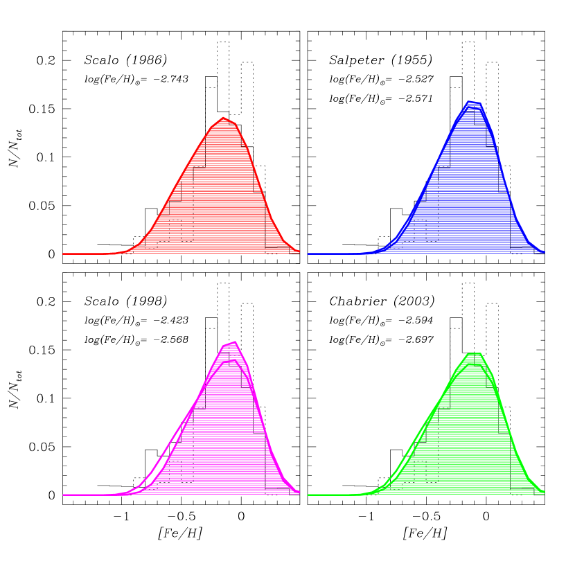
Figure 4: Theoretical G-dwarf metallicity distribution as predicted by the model with Maeder & Meynet (1989) stellar lifetimes and different assumptions on the IMF (thick lines) compared to the data (histograms; solid: Rocha-Pinto & Maciel 1996; dotted: Jørgensen 2000). Theoretical [Fe/H] are normalized to the iron to hydrogen ratios predicted by the model at Sun’s birth, which are displayed in the upper left corner of each panel. The first value refers to a common choice for the parameter regulating the fraction of stars giving rise to SNIa events, $A$ = 0.05; the second value refers to the case in which the $A$ parameter is adjusted so as to predict the same SNIa rate at the present time when changing the IMF (see text for details). The theoretical distributions corresponding to the latter case are shown as dashed areas. Remember that SNeIa are the major iron producers in the Milky Way. Notice that theoretical distributions are convolved with a Gaussian in order to account for both the observational and the intrinsic scatter.

Also shown are data from Rocha-Pinto & Maciel (1996; thin solid histograms) and Jørgensen (2000; thin dotted histograms). The two distributions look quite different. In the case of Jørgensen’s, the peak is shifted to higher metallicities and the low-metallicity tail is almost absent, similarly to what found by Wyse & Gilmore (1995). This is because of the different metallicity calibrations and the different corrections to the raw data applied by the authors. Indeed, in Rocha-Pinto & Maciel (1996) the metallicity scale is biased towards metal-poor stars (Martell & Laughlin 2002). This determines a shift of the peak of the distribution towards lower metallicities. The actual peak position is likely to be more near $-0.15$ dex than $-0.25$ dex (H. Rocha-Pinto, private communication), thus bringing model predictions and observational distributions in better agreement.

Table 3: Type Ia SN rates and Type Ia to Type II SN rate ratios at the present time predicted by the model with different IMFs. All the IMFs are normalized to the mass range 0.1–100 $M_{\odot}$. The value of the parameter $A$, determining the stellar mass fraction belonging to binary systems with the right characteristics to give rise to SNIa explosions, is the same independently of the adopted IMF. Observed values are from van den Bergh & Tammann (1991) and Cappellaro et al. (1997).

$\mathrm{IMF}$	$A$	$R_{\mathrm{Ia}}\;{\mathrm{(century^{-1})}}$	$R_{\mathrm{Ia}}/R_{\mathrm{II}}$
${\mathrm{S55}}$	$0.05$	$0.57$	$0.34$
${\mathrm{T80}}$	$0.05$	$1.16$	$0.30$
${\mathrm{S86}}$	$0.05$	$0.45$	$0.46$
${\mathrm{K93}}$	$0.05$	$0.67$	$0.38$
${\mathrm{S98}}$	$0.05$	$1.03$	$0.26$
${\mathrm{C03}}$	$0.05$	$0.69$	$0.34$
${\mathrm{Observed}}$		$0.6\;h^{2}$	$0.15$–$0.27$

S55 – Salpeter (1955); T80 – Tinsley (1980); S86 – Scalo (1986); K93 – Kroupa et al. (1993); S98 – Scalo (1998); C03 – Chabrier (2003) with $x$ = 1.7.

Table 4: Same as Table 3, but changing the value of $A$ to recover the same SNIa rate at the present time with different IMFs.

$\mathrm{IMF}$	$A$	$R_{\mathrm{Ia}}\;{\mathrm{(century^{-1})}}$	$R_{\mathrm{Ia}}/R_{\mathrm{II}}$
${\mathrm{S55}}$	$0.04$	$0.47$	$0.27$
${\mathrm{T80}}$	$0.02$	$0.46$	$0.17$
${\mathrm{S86}}$	$0.05$	$0.45$	$0.46$
${\mathrm{K93}}$	$0.035$	$0.45$	$0.25$
${\mathrm{S98}}$	$0.023$	$0.47$	$0.12$
${\mathrm{C03}}$	$0.032$	$0.43$	$0.23$
${\mathrm{Observed}}$		$0.6\;h^{2}$	$0.15$–$0.27$

S55 – Salpeter (1955); T80 – Tinsley (1980); S86 – Scalo (1986); K93 – Kroupa et al. (1993); S98 – Scalo (1998); C03 – Chabrier (2003) with $x$ = 1.7.

It is worth reminding that iron originates mostly from SNIa explosions occurring in binary systems with an intermediate-mass primary. Only one third of its solar abundance is related to SNII events, occurring on much shorter time scales. Therefore, the stars responsible for the observed behaviour of the iron abundance belong mostly to the 1.5–8 $M_{\odot}$ stellar mass range, that is the one characterizing Type Ia SN progenitors in our model.

For each stellar generation, the mass fraction in form of binaries having the right characteristics to end up as SNeIa is a free parameter of the model, whose value is kept constant in time. Following Matteucci & Greggio (1986), the rate of Type Ia SNe is:

$$R_{\mathrm{Ia}}(t)=A\int_{m_{B_{\mathrm{m}}}}^{m_{B_{\mathrm{M}}}}\varphi(m_{B})\bigg{[}\int_{\mu_{\mathrm{m}}}^{0.5}f(\mu)\psi(t-\tau_{m_{2}}){\mathrm{d}}\mu\bigg{]}{\mathrm{d}}m_{B},$$

where $\varphi(m_{B})$ is the IMF for the total mass of the binary system; $f(\mu)$ is the distribution function for the mass fraction of the secondary component ($\mu$ = $m_{2}/m_{B}$); $\tau_{m_{2}}$ is the lifetime of the secondary; $m_{B_{\mathrm{m}}}$ = 3 $M_{\odot}$ and $m_{B_{\mathrm{M}}}$ = 16 $M_{\odot}$ (see Matteucci & Recchi 2001 for a review and alternative formulations). The parameter $A$ is fixed by the request of reproducing the SNIa rate currently observed in the disk. Moreover, the ratio $R_{\mathrm{Ia}}/R_{\mathrm{II}}$ between the Type Ia and II SN rates in the solar vicinity should be reproduced.

Table 5: Abundances in the Protosolar Cloud as predicted by the model at $t$ = 9.2 Gyr with different assumptions on the IMF. The abundances are by number in $\log\varepsilon$(X), except for helium ($Y$) and global metallicity ($Z$), for which the abundances by mass are reported. Model predictions are compared to observed photospheric solar abundances, unless otherwise stated.

$\mathrm{IMF}$	$Y$	${\mathrm{C}}$	${\mathrm{N}}$	${\mathrm{O}}$	${\mathrm{Ne}}$	${\mathrm{Mg}}$	${\mathrm{Si}}$	${\mathrm{S}}$	${\mathrm{Fe}}$	$Z$
${\mathrm{S55a}}$	$0.264$	$8.53$	$8.33$	$9.12$	$8.27$	$7.55$	$7.81$	$7.39$	$7.68$	$0.028$
${\mathrm{T80a}}$	$0.273$	$8.56$	$8.46$	$8.98$	$8.07$	$7.39$	$7.82$	$7.40$	$7.71$	$0.024$
${\mathrm{S86a}}$	$0.260$	$8.36$	$8.04$	$8.77$	$7.84$	$7.14$	$7.52$	$7.11$	$7.51$	$0.014$
${\mathrm{K93a}}$	$0.264$	$8.46$	$8.18$	$8.87$	$7.97$	$7.27$	$7.62$	$7.21$	$7.55$	$0.017$
${\mathrm{S98a}}$	$0.271$	$8.64$	$8.49$	$9.18$	$8.36$	$7.64$	$7.87$	$7.44$	$7.68$	$0.033$
${\mathrm{C03a}}$	$0.265$	$8.48$	$8.21$	$8.89$	$8.00$	$7.30$	$7.64$	$7.23$	$7.55$	$0.018$
${\mathrm{C03b}}$	$0.263$	$8.44$	$8.15$	$8.85$	$7.95$	$7.25$	$7.60$	$7.19$	$7.54$	$0.017$
${\mathrm{Observations}}$
${\mathrm{GS98}}$	$0.275\pm 0.01$	$8.52\pm 0.06$	$7.92\pm 0.06$	$8.83\pm 0.06$	$8.08\pm 0.06^{\mathrm{a}}$	$7.58\pm 0.05$	$7.55\pm 0.05$	$7.33\pm 0.11$	$7.50\pm 0.05$	$0.017$
${\mathrm{H01}}$		$8.59\pm 0.11$	$7.93\pm 0.11$	$8.74\pm 0.08$		$7.54\pm 0.06$	$7.54\pm 0.05$		$7.45\pm 0.08$
${\mathrm{AP01}}$				$8.69\pm 0.05$
${\mathrm{AP02}}$		$8.39\pm 0.04$
${\mathrm{A04}}$				$8.66\pm 0.05$	$7.84\pm 0.06$					$0.0126$

• Coronal data.

S55 – Salpeter (1955); T80 – Tinsley (1980); S86 – Scalo (1986); K93 – Kroupa et al. (1993); S98 – Scalo (1988); C03 – Chabrier (2003) with $x$ = 1.7. The letter refers to the adopted normalization range: a stands for 0.1–100 $M_{\odot}$; b for 0.001–100 $M_{\odot}$. GS98 – Grevesse & Sauval (1998); H01 – Holweger (2001); AP01 – Allende Prieto et al. (2001); AP02 – Allende Prieto et al. (2002); A04 – Asplund et al. (2004).

In Table 3 we list the present-day values of $R_{\mathrm{Ia}}$ and $R_{\mathrm{Ia}}/R_{\mathrm{II}}$ which are predicted by assuming different IMFs, while keeping the value of $A$ constant (the often quoted value of 0.05 for $A$ is adopted). If $h$ = 0.7 and a factor of two of uncertainty in the observations is assumed, it turns out that both a Tinsley (1980) and a Scalo (1998) IMF provide only a marginal agreement with the observed SNIa rate. The reason for this is that, among all the studied IMFs, Tinsley’s (1980) and Scalo’s (1998) are those allocating the highest mass fraction to the stellar mass range 1.5–8 $M_{\odot}$, typical of SNIa progenitors.

Table 4 illustrates what happens if the value of $A$ is adjusted so as to bring the value of $R_{\mathrm{Ia}}$ in agreement with the observations when changing the IMF. The corresponding G-dwarf metallicity distributions are shown in Fig. 4 (dashed areas). Lowering $A$ from 0.05 to 0.04, 0.023 and 0.032, in case of Salpeter (1955), Scalo (1998) and Chabrier (2003) IMF, respectively, results in narrower, more peaked distributions. Nevertheless, after convolution with a Gaussian accounting for the observational and intrinsic error, the differences almost completely level off. The agreement with the observations is always satisfactory. The Chabrier IMF also gives a good fit to the $R_{\mathrm{Ia}}/R_{\mathrm{II}}$ ratio currently observed in the solar vicinity. For the Scalo (1986) IMF, a better value for the $R_{\mathrm{Ia}}/R_{\mathrm{II}}$ ratio can be obtained by further reducing the $A$ value. The Kroupa et al. (1993) IMF is an equally valid choice. However, no firm conclusions can be drawn on the grounds of the SN rates, given the high uncertainty level still affecting the data. In what follows, for each IMF we discuss the results obtained with the corresponding $A$ value listed in Table 4, unless otherwise specified.

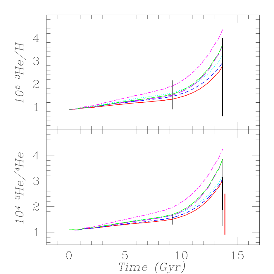
Figure 5: Upper panel: evolution of ³He/H in the solar neighbourhood. Different lines refer to different IMF prescriptions: short-dashed line: Salpeter (1955); dotted line: Tinsley (1980); continuous line: Scalo (1986); long-dashed line: Kroupa et al. (1993); dot-short-dashed line: Scalo (1998); dot-long-dashed line: Chabrier (2003) with $x$ = 1.7 for $m>$ 1 $M_{\odot}$. Data (vertical bars at $t$ = 9.2 and 13.7 Gyr) are from Geiss & Gloeckler (1998). Lower panel: evolution of ³He/⁴He in the solar neighbourhood. Models are labeled as in the upper panel. Data are from Geiss & Gloeckler (1998; at 1 and 2 $\sigma$ – thick and thin vertical bars, respectively, at $t$ = 9.2 and 13.7 Gyr) and Salerno et al. (2003; 1 $\sigma$-bar on the right at $t$ = 13.7 Gyr).

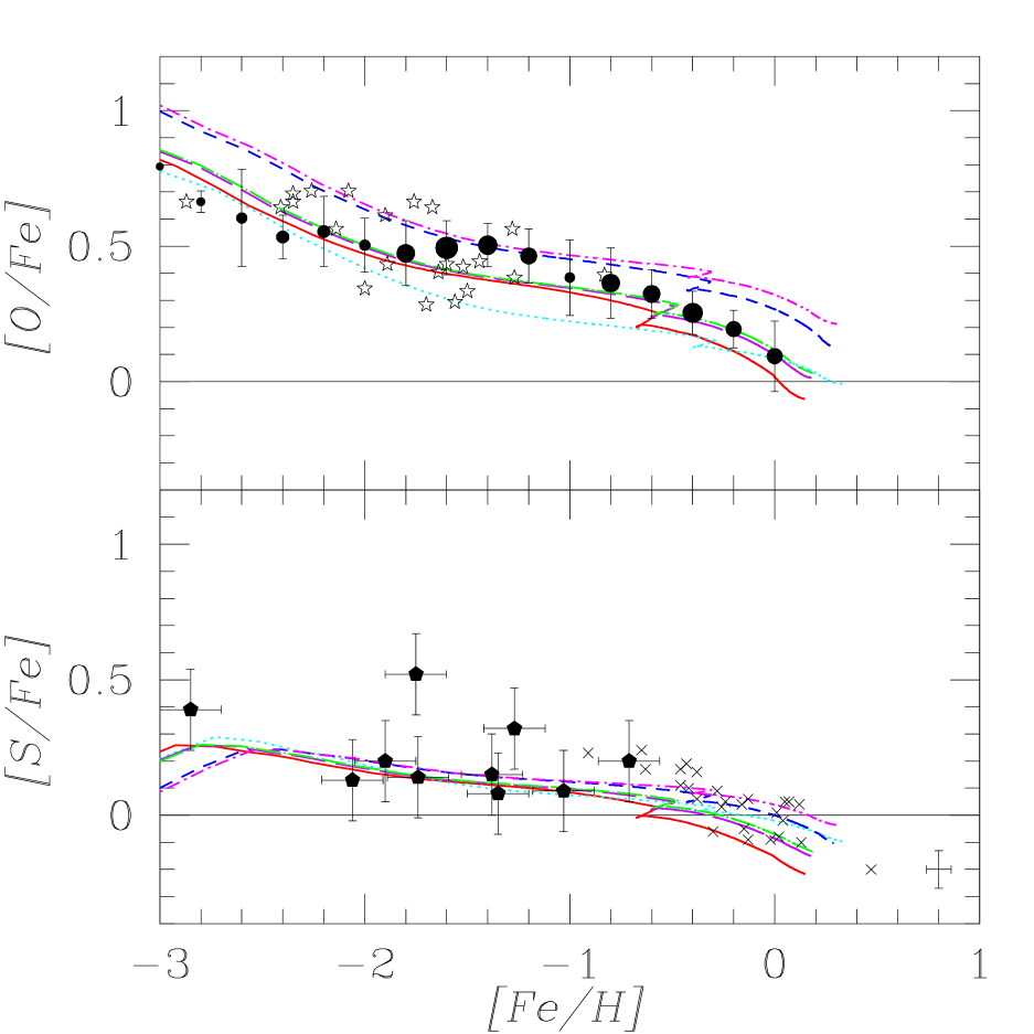
Figure 6: [O/Fe] (upper panel) and [S/Fe] (lower panel) ratios as functions of [Fe/H]. Models as in Fig. 5. All the ratios are normalized to solar elemental abundances by Grevesse & Sauval (1998), except for oxygen, for which the solar value from Holweger (2001) is adopted. Data for oxygen are from Meléndez & Barbuy (2002; stars: [O/Fe] values from infrared OH lines; full circles: mean [O/Fe] from [O I] line in bins of 0.2 dex in [Fe/H]; the size of the circles represents the number of stars in each metallicity bin). Data for sulphur are from Ryde & Lambert (2004; pentagons: measurements from observations of S I lines at 9212.9, 9228.1 and 9237.5 Å) and Chen et al. (2002; crosses). For these latter measurements, the typical error is also reported on the lower right corner of the panel.

In Table 5 we display the abundances of ⁴He, C, N, O, Ne, Mg, Si, S, Fe and the global metallicity, $Z$, predicted by the model at the time of the Solar System formation 4.5 Gyr ago, under different prescriptions on the IMF. Theoretical values are compared to observed ones from Grevesse & Sauval (1998), Holweger (2001), Allende Prieto, Lambert & Asplund (2001, 2002) and Asplund et al. (2004). One may wonder whether the use of the Sun as representative of the chemical composition of the ISM of the local disc 4.5 Gyr ago is suitable for comparison with GCE model predictions. Indeed, the empirical age-metallicity relationship for solar neighbourhood stars shows a large dispersion (Edvardsson et al. 1993), with known planet-harbouring stars being systematically more metal rich than stars without planets (Ibukiyama & Arimoto 2002, their figure 21). On the other hand, a recent reappraisal of the chemical composition of the Orion nebula suggests heavy element abundances only slightly higher ($\sim$ 0.1 dex) than the solar ones, in agreement with GCE model predictions, challenging the view that the Sun has abnormally high metal abundances (Esteban et al. 2004).

It is seen that a model adopting Tinsley (1980) or Scalo (1998) IMF is in better agreement with the solar helium mass fraction (see also Romano et al. 2003), but overestimates the overall metallicity of the gas and the iron content. This is due to the high stellar mass fraction distributed over the mass range 2–40 $M_{\odot}$ according to these IMFs (see Table 1), coupled with the high helium and global metal yields predicted in this mass range by stellar evolution theory (see figures 2.9, 2.10 of Matteucci 2001). Trying to reduce the predicted solar iron abundance by further lowering the $A$ parameter is not a viable solution (although at first glance it could appear as a very simple and promising one), since a too low $R_{\mathrm{Ia}}/R_{\mathrm{II}}$ ratio would be obtained in this case, in disagreement with the available data. Notice that a better agreement with the ⁴He data can be achieved by model S86a if adopting the ⁴He yields recently computed by Meynet & Maeder (2002), which include mass loss and rotation in self-consistent stellar evolutionary models. Indeed, a value of 0.272 for $Y$ at the time of Sun formation is predicted in this case, in very good agreement with the observed solar value (Chiappini, Matteucci & Meynet 2003b).

Salpeter’s IMF also predicts far too high values for the solar abundances of iron, oxygen and metals in general, because of its high percentage of massive stars (see also Tosi 1988, 1996). In particular, with this IMF and the star formation law adopted here, there happens to be no way to reconcile the theoretical solar abundances with the observed ones, unless one requires a SF process so unefficient that severe discrepancies with other observational constraints do arise. In particular, by using $\nu\sim$ 0.2 Gyr^-1 in the SFR expression reported in Section 4, the model matches the actual metallicity of the Sun, but underestimates the present-day stellar mass density in the solar vicinity. In fact, in this case the expected stellar mass density at the present time turns out to be $\Sigma_{\mathrm{stars}}(t_{\mathrm{Gal}})\simeq$ 22 $M_{\odot}$ pc^-2, to be compared with an observed value of 35 $\pm$ 5 $M_{\odot}$ pc^-2.

The nitrogen solar abundance is overestimated by all the models, except by the model assuming Scalo’s (1986) IMF. This same model also predicts a solar carbon abundance in good agreement with the observations, if one believes that the solar photospheric abundance from Allende Prieto et al. (2002) gives the best estimate of carbon in the Sun. A model assuming Kroupa et al. or Chabrier’s IMF also agrees with the CNO data, but only at the 2-$\sigma$ level. However, it should be noticed that: (i) the nitrogen and carbon yields from low- and intermediate-mass stars are very uncertain and (ii) the carbon yields from stars with $m>$ 40 $M_{\odot}$ have been multiplied by a factor of three in order to mimic results from recent models taking mass loss and stellar rotation into account (see Chiappini et al. 2003a, b and references therein) and both of these mechanisms are still far from being fully understood. In conclusion, it is likely that the uncertainties in the stellar nucleosynthesis are the most important sources of errors as far as both carbon and nitrogen evolution are concerned.

The effect of extending the lognormal form of the IMF derived by Chabrier (2003) for $m<$ 1 $M_{\odot}$ to the BD domain is also studied. BDs are low-mass, long-living objects, that act simply as sinks of matter from the point of view of galactic chemical evolution. They were born at every time of Galaxy’s evolution and never restored matter into the ISM. According to what reported in Table 2, only a small fraction ($<$ 10%) of the total mass of a stellar generation should be locked up in BDs. Therefore, only small effects are expected to appear when extending the IMF to the BD domain. This is what is actually found (compare model C03a to model C03b results in Table 5). Nevertheless, considering the existence of a substellar mass regime reduces the amount of matter processed through nuclear burning in stars during the whole Galactic lifetime. This results in lower abundances in the gaseous matter at the time of Sun’s formation, thus obtaining a better agreement with the observations. The current stellar density we obtain in the solar neighbourhood in the two cases is fairly similar, being $\Sigma_{\mathrm{stars}}(t_{\mathrm{Gal}})\simeq$ 34 $M_{\odot}$ pc^-2 if BDs are not taken into account and $\Sigma_{\mathrm{stars}}(t_{\mathrm{Gal}})\simeq$ 29 $M_{\odot}$ pc^-2 if they are. Both values are within the errors associated with the observational estimate, though the higher value is more likely.

Figs. 5 and 6 show the errors associated with chemical evolution model predictions for several quantities, obtained by changing the prescriptions for the stellar IMF and keeping the same stellar lifetimes (Maeder & Meynet 1989). Model predictions on the evolution of ³He/H and ³He/⁴He as functions of time (Fig. 5, upper and lower panel, respectively) and [O/Fe] and [S/Fe] as functions of [Fe/H] (Fig. 6, upper and lower panel, respectively) in the solar neighbourhood are shown, as well as the corresponding data. Model predictions are not normalized to the predicted solar values, as instead is often done in chemical evolution studies. This is to better appreciate the differences obtained with the various IMFs in the last 4.5 Gyr of evolution, an effect which is not evident when the solar normalization is applied. The elements displayed in Figs. 5 and 6 are not chosen randomly. They are representative of stellar progenitors belonging to different initial mass ranges: (i) ³He is produced by stars belonging to the low-mass range, 1–2 $M_{\odot}$; (ii) ⁴He comes from the whole stellar mass range; (iii) oxygen is almost entirely produced on short time scales by stars with $m>$ 10 $M_{\odot}$; (iv) sulphur is representative of elements produced partly by SNeII and partly by SNeIa; finally, (v) Fe is mostly produced by Type Ia SNe on long timescales.

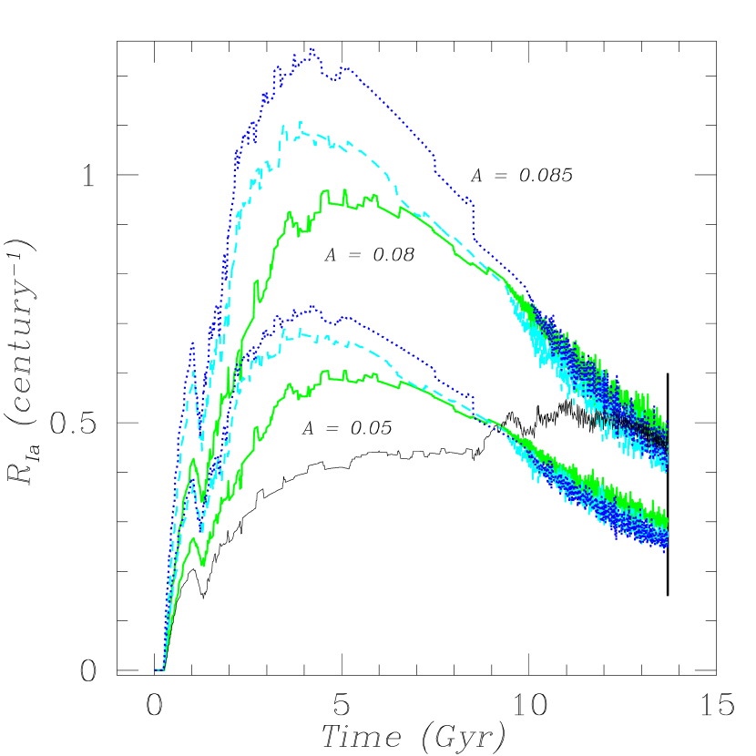
Figure 7: Type Ia SN rates obtained with different assumptions on the stellar lifetimes (Maeder & Meynet 1989 – thin solid line; Tinsley 1980 – thick dotted line; Schaller et al. 1992 – thick solid line; Kodama 1997 – thick dashed line). We also show the effect of changing the fraction of mass entering the formation of Type Ia SN progenitors. The four curves lying in the lower part of the diagram have all been computed with $A$ = 0.05, while the value of $A$ for the curves lying in the upper part of the diagram has been changed so as to produce the same present-day $R_{\mathrm{Ia}}$ in the disk, independently of the adopted stellar lifetime prescriptions. The Type Ia SN rate observed in the Galaxy at the present time is also shown (vertical bar, for $h$ = 0.7; Cappellaro et al. 1997).

Table 6: Abundances in the PSC as predicted by the model at $t$ = 9.2 Gyr for different assumptions on the stellar lifetimes. The abundances are by number in $\log\varepsilon$(X), except for helium ($Y$) and global metallicity ($Z$), for which the abundances by mass are reported. Model predictions are compared to observed photospheric solar abundances, unless otherwise stated. A value of $A$ = 0.05 is assumed for all models (see text).

$\tau_{m}$	$Y$	${\mathrm{C}}$	${\mathrm{N}}$	${\mathrm{O}}$	${\mathrm{Ne}}$	${\mathrm{Mg}}$	${\mathrm{Si}}$	${\mathrm{S}}$	${\mathrm{Fe}}$	$Z$
${\mathrm{T80}}$	$0.261$	$8.39$	$8.13$	$8.90$	$7.97$	$7.23$	$7.57$	$7.18$	$7.57$	$0.017$
${\mathrm{M89}}$	$0.260$	$8.36$	$8.04$	$8.77$	$7.84$	$7.14$	$7.52$	$7.11$	$7.51$	$0.014$
${\mathrm{S92}}$	$0.260$	$8.36$	$8.06$	$8.80$	$7.89$	$7.17$	$7.55$	$7.10$	$7.54$	$0.015$
${\mathrm{K97}}$	$0.260$	$8.35$	$8.08$	$8.81$	$7.89$	$7.17$	$7.51$	$7.11$	$7.56$	$0.015$
${\mathrm{Observations}}$
${\mathrm{GS98}}$	$0.275\pm 0.01$	$8.52\pm 0.06$	$7.92\pm 0.06$	$8.83\pm 0.06$	$8.08\pm 0.06^{\mathrm{a}}$	$7.58\pm 0.05$	$7.55\pm 0.05$	$7.33\pm 0.11$	$7.50\pm 0.05$	$0.017$
${\mathrm{H01}}$		$8.59\pm 0.11$	$7.93\pm 0.11$	$8.74\pm 0.08$		$7.54\pm 0.06$	$7.54\pm 0.05$		$7.45\pm 0.08$
${\mathrm{AP01}}$				$8.69\pm 0.05$
${\mathrm{AP02}}$		$8.39\pm 0.04$
${\mathrm{A04}}$				$8.66\pm 0.05$	$7.84\pm 0.06$					$0.0126$

• Coronal data.

T80 – Tinsley (1980); M89 – Maeder & Meynet (1989); S92 – Schaller et al. (1992); K97 – Kodama (1997); GS98 – Grevesse & Sauval (1998); H01 – Holweger (2001); AP01 – Allende Prieto et al. (2001); AP02 – Allende Prieto et al. (2002); A04 – Asplund et al. (2004).

Scalo’s (1998) IMF, having the highest fractions of stars with $m>$ 10 $M_{\odot}$ and 1 $\leq m/M_{\odot}\leq$ 2 (Fig. 1), predicts a too large O/Fe ratio during the whole Galactic lifetime and an increase of ³He/H and ³He/⁴He from the time of Sun’s formation up to now that hardly fits the data. This is because the stars in the range 1–2 $M_{\odot}$ are net ³He producers, even when $\sim$90% of them are assumed to experience the cool bottom processes which strongly deplete their ³He yields (see next section for more details and references), whereas high-mass stars produce almost all the oxygen. On the contrary, Salpeter, Tinsley and Scalo (1986) IMFs predict enrichment histories for ³He/H and ³He/⁴He which better agree with the data, because of the lower mass fraction falling in the 1–2 $M_{\odot}$ stellar mass range. The Kroupa et al. and Chabrier IMFs, with $x$ = 1.7 for $m>$ 1 $M_{\odot}$, produce an intermediate behaviour. They also guarantee the best fit to the [O/Fe] vs [Fe/H] data. The (small) differences in the S/Fe ratio in the disc are mostly related to the (slightly) different behaviour of the SNIa rate in the past predicted when adopting different IMFs.

5.2 Changing the stellar lifetimes

In this section we keep fixed the prescriptions on the stellar IMF, while varying those on the stellar lifetimes, according to what has been reviewed in Section 3. We choose to adopt Scalo (1986) IMF for the sake of comparison with previous results published in a series of papers dealing with different aspects of the Milky Way evolution (e.g. Chiappini et al. 1997; Romano et al. 2003, and references therein).

In the following, we compare results of chemical evolution models for the solar vicinity adopting stellar lifetimes from: (i) Tinsley (1980); (ii) Maeder & Meynet (1989); (iii) Schaller et al. (1992); (iv) Kodama (1997).

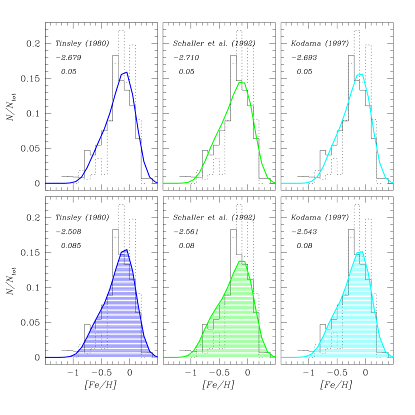
Figure 8: Theoretical G-dwarf metallicity distributions (thick lines) predicted by the model with different assumptions on the stellar lifetimes (left panels: Tinsley 1980; middle panels: Shaller et al. 1992; right panels: Kodama 1997) and on the fraction of mass entering the formation of Type Ia SN progenitors (upper panels: $A$ = 0.05; lower panels: $A$ = 0.08 in case of Schaller et al.’s and Kodama’s stellar lifetimes; $A$ = 0.085 in case of Tinsley’s stellar lifetimes). Scalo’s (1986) IMF is assumed in all cases. Theoretical distributions are compared to observational ones from Rocha-Pinto & Maciel (1996; solid histograms) and Jørgensen (2000; dotted histograms). For each model, the theoretical [Fe/H] ratios are normalized to the Fe/H ratio at Sun’s birth predicted by the model itself, given in the upper left corner of each panel (middle row). This produces a shift of the distribution along the x axis, thus allowing for a better comparison of the theoretical shape with the observed one even if the model does not recover the actual iron abundance of the Sun.

In Chiappini et al. (1997) and subsequent work by that group, the prescriptions of Maeder & Meynet (1989) were adopted. According to those authors, stars with 1.3 $\leq m/M_{\odot}\leq$ 3 are characterized by lifetimes longer than in any other study (see Fig. 3). This causes the Type Ia SN rate to increase smoothly during almost the whole disk evolution, with a gentle decline starting only a couple of Gyrs ago (thin solid line in Fig. 7). On the contrary, models with different prescriptions on the stellar lifetimes all produce a well-defined peak in the rate, followed by a steep decline afterward (thick lines in Fig. 7). If one adopts Tinsley’s (1980), Schaller et al.’s (1992) or Kodama’s (1997) stellar lifetimes, keeping $A$ – i.e. the fraction of mass belonging to binary systems which will give rise to Type Ia SN explosions – constant and equal to 0.05 results in a little bit more iron produced until the time of Sun’s formation (see also Table 6, column 10), while SNeIa are supposed to be less numerous in the disk at the present time. However, their number still agrees with that inferred from the observations (vertical bar in Fig. 7). To rise the present-day SNIa rate to the value expected when adopting Maeder & Meynet (1989) stellar lifetimes, it is necessary to increase the fraction of mass belonging to SNIa progenitors. In particular, when adopting Schaller et al. (1992) or Kodama (1997) $\tau_{m}$s, $A=0.08$ is required, while a slightly higher value, $A=0.085$, must be assumed if Tinsley’s (1980) stellar lifetimes are adopted (upper curves in Fig. 7). Increasing the efficiency of star formation while leaving the $A$ parameter unchanged would also lead to an increase of the SNIa rate, but it would also cause major problems in reproducing other important constraints available for the immediate solar vicinity. From Fig. 7 and Table 6, column 10, we conclude that, for a Scalo (1986) IMF, a small $A$ value of the order of 0.05 or even less should be preferred, because it produces theoretical predictions matching remarkably well the solar iron abundance and the present-day SNIa rate data at the same time.

The G-dwarf metallicity distributions obtained with all the above-mentioned prescriptions for $\tau_{m}$ are displayed in Figs. 4 (upper left panel) and 8. Again, the theoretical distributions are convolved with a Gaussian to account for both the observational and the intrinsic scatter. The adopted total dispersion in [Fe/H] is $\sigma$ = 0.15 dex (Arimoto, Yoshii & Takahara 1992; Kotoneva et al. 2002). Since most of the iron in the solar neighbourhood comes from Type Ia SNe, the shape of the distribution is expected to change according to changes affecting Type Ia SN progenitors. Indeed, adopting Tinsley (1980) or Kodama (1997) stellar lifetimes (Fig. 8, left and right panels, respectively) results in a more pronounced peak, independently of the value of $A$ (which is given in the upper left corner of each panel, third row).

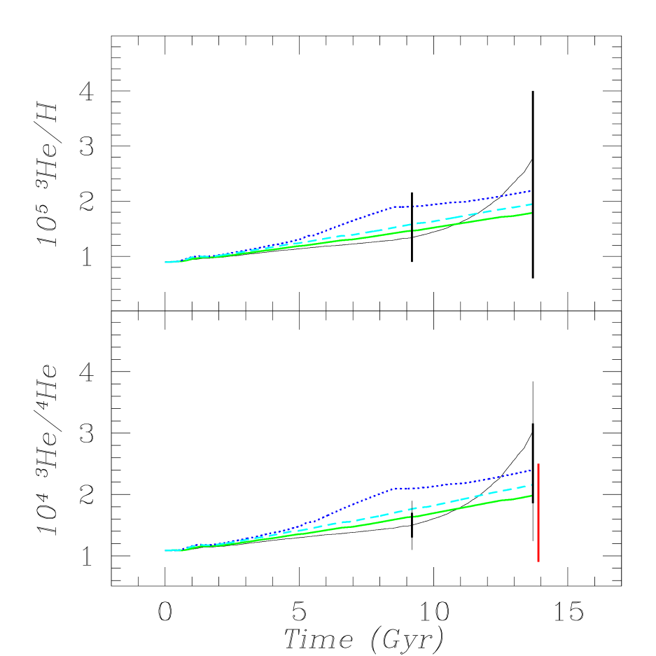
Figure 9: Same as Fig. 5, but here different line types refer to different prescriptions on the stellar lifetimes. Thin solid lines: Maeder & Meynet (1989); thick solid lines: Schaller et al. (1992); thick dotted lines: Tinsley (1980); thick dashed lines: Kodama (1997). The Scalo (1986) IMF is assumed for all the models.

It is worth noticing that, independently of the choice of the stellar lifetimes, we always get a strikingly good fit to the position of the peak and to the high-metallicity tail of the distribution. We conclude that: (i) the main parameter driving the location of the peak and the shape of the distribution is the adopted time scale for thin-disk formation, which was already well known (Chiappini et al. 1997); (ii) the adopted stellar lifetimes affect the theoretical G-dwarf distribution as well, though through a second order effect: they mostly act on the width and height of the distribution. However, convolution with a Gaussian which accounts for errors makes different distributions, obtained with different prescriptions on the stellar lifetimes, look pretty much the same.

In Table 6 we report the abundances in the Protosolar Cloud (PSC) predicted under different assumptions on the stellar lifetimes. Notice that for all the models in Table 6 a value of 0.05 for $A$ is adopted. A larger $A$ value would overestimate the iron content of the Sun. It can be seen that the global metallicity, $Z$, is well reproduced by all the models and so are the CNO abundances, with a possible exception for oxygen, whose predicted solar abundance is a bit higher than observed. On the other hand, the helium abundance turns out to be too low. Increasing the star formation efficiency would provide a higher $Y$ abundance, but the oxygen and global metallicity would also increase, breaking the agreement with the observations. This clearly shows that some revision on the helium stellar yields is necessary (see Meynet & Maeder 2002; Chiappini et al. 2003b).

Let us now comment on specific trends predicted for a handful of important species: (i) ³He and (ii) ⁷Li, coming mostly from low-mass stellar progenitors; (iii) oxygen, a typical massive star product; and (iv) sulphur, with both a SNII and a SNIa component. Major differences are expected in the model predictions for ³He and ⁷Li, because of the large differences characterizing different $\tau_{m}$ prescriptions for their stellar progenitors.

To deal with ³He, one must keep in mind that it is mostly produced by low-mass – hence long-living – stars. Standard stellar evolutionary theory predicts a large production of ³He from low-mass stars leading to severe inconsistency between the observed ³He abundances and those predicted by chemical evolution models assuming these standard yields (Rood, Steigman & Tinsley 1976; Galli et al. 1995; Olive et al. 1995; Dearborn et al. 1996; Prantzos 1996). A problem that has been now superseeded by the inclusion of rotational mixing in stellar models (e.g. Charbonnel 1995; Sackmann & Boothroyd 1999). Indeed, extra mixing makes it possible to reconcile predictions from Galactic chemical evolution models with observations, as long as ³He is destroyed in a large enough fraction ($\sim$90%) of low-mass stars (e.g. Galli et al. 1997; Chiappini et al. 2002, and references therein). Fig. 9 shows the ³He evolution in the solar neighbourhood as predicted under different assumptions on the stellar lifetimes: the thin solid lines are for Maeder & Meynet (1989); the thick solid lines are for Schaller et al. (1992); the thick dotted lines for Tinsley (1980) and the thick dashed ones for Kodama (1997). The prescriptions on ³He synthesis are those from Dearborn et al. (1996) and Sackmann & Boothroyd (1999) for stars without and with extra-mixing. These ³He yields were recently adopted also by Chiappini et al. (2002) and Romano et al. (2003) and take extra-mixing in 93% of low-mass stars into account. The lower ³He production for $t<$ 11–12 Gyr predicted assuming Maeder & Meynet (1989) stellar lifetimes is due to the longer lifetimes in the mass range 1–2 $M_{\odot}$. The subsequent steep rise is mostly due to the late contribution from stars in the 0.6–0.9 $M_{\odot}$ mass range, which die if adopting the Matteucci & François (1989) extrapolation of Maeder & Meynet’s stellar lifetimes in the very low stellar mass range. Conversely, these stars never die if the Schaller et al., Tinsley or Kodama stellar lifetimes are adopted instead (Fig. 3; see also the discussion in Romano et al. 2003). If one trusts the local value of the helium isotopic ratio as measured with the COLLISA experiment on board the space station MIR (Salerno et al. 2003 – Fig. 9, lower panel, vertical bar on the right at $t$ = 13.7 Gyr), longer lifetimes for stars with $m<$ 1 $M_{\odot}$ should be preferred. In fact, this measurement supports the hypothesis that negligible changes of the abundance of ³He occurred in the Galaxy during the last 4.5 Gyr.

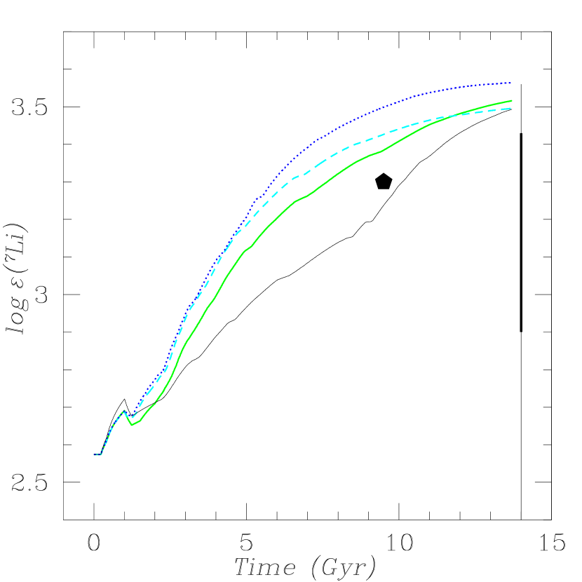
Figure 10: Temporal evolution of lithium in the solar neighbourhood. Different curves refer to model predictions obtained with different recipes for the stellar lifetimes. Thin solid line: Maeder & Meynet (1989); thick solid line: Schaller et al. (1992); thick dotted line: Tinsley (1980); thick dashed line: Kodama (1997). The meteoritic (Nichiporuk & Moore 1974; pentagon) and the depletion corrected value for the local ISM (Knauth et al. 2003; at 1- and 2-$\sigma$ – thick and thin vertical bars, respectively) are shown as well. Notice that the $\alpha$ value (where $\alpha$ is the fraction of white dwarfs entering the formation of nova systems) is adjusted so as to reproduce the nova outburst rate currently observed in the Galaxy. In particular, in the case of Tinsley, Schaller et al. and Kodama stellar lifetimes $\alpha\sim$ 0.02, while $\alpha\sim$ 0.01 if Maeder & Meynet stellar lifetimes are adopted instead (see text for details).

Lithium is another element originating mostly from low-mass stars (Romano et al. 2001). According to our models, its meteoritic abundance is due for $\sim$40% to low-mass ($m$ = 1–2 $M_{\odot}$) stars on the red giant branch (RGB) and for $\sim$10% to novae, binary systems consisting of a white dwarf plus a main sequence companion (Romano et al. 2001, 2003; but see also Casuso & Beckman 2000 and Travaglio et al. 2001 for different views). The predicted steep rise of the lithium abundance in the ISM at late times is dictated by the long time scales for lithium production from RGB stars and novae when adopting Maeder & Meynet stellar lifetimes. Here we analyse what changes are introduced by adopting different stellar lifetimes. In Fig. 10, we compare model predictions for the temporal evolution of ⁷Li in the solar vicinity obtained by adopting Maeder & Meynet (1989) stellar lifetimes (thin solid line) to what we get if adopting Schaller et al. (1992 – thick solid line), Tinsley (1980 – thick dotted line) or Kodama (1997– thick dashed line) prescriptions. The Schaller et al. stellar lifetimes result in a more gentle rise during the last $\sim$ 3 Gyrs, while almost no evolution is expected during the same time interval with Tinsley (1980) or Kodama (1997) prescriptions. These considerations read interesting in the light of recent claims of a null ⁷Li evolution in the ISM during the last several Gyrs inferred from cluster and field star lithium data (Lambert & Reddy 2004). However, in our opinion these data do not rule out a scenario of late lithium pollution from low-mass stars, if the uncertainties in both the models and the data are properly taken into account.

In our model, nearly 10% of lithium in meteorites is produced during nova outbursts. These are periodical explosions, that do not destroy the parent system. When dealing with nova systems, one must introduce in the model a free parameter, $\alpha$, describing the fraction of white dwarfs which enters the formation of nova systems (similarly to what is done for SNeIa; see D’Antona & Matteucci 1991; Romano et al. 1999; Matteucci et al. 2003). Fig. 10 shows model results obtained by changing the $\alpha$ value so as to obtain the same theoretical nova outburst rate in the Galaxy at the present time, whatever the $\tau_{m}$ choice. A value of $R_{\mathrm{nova}}(t_{\mathrm{Gal}})\simeq$ 20 yr^-1 is found with $\alpha\sim 0.01$ in the case of Maeder & Meynet stellar lifetimes and $\alpha\sim 0.02$ in the remaining cases, to be compared with $R_{\mathrm{nova}}^{\mathrm{obs}}=$ 20–30 yr^-1 (Shafter 1997). When using Tinsley’s, Schaller et al.’s or Kodama’s stellar lifetimes, a ⁷Li production from novae higher than expected when using Maeder & Meynet’s stellar lifetimes is obtained during the whole Galactic lifetime, owing to the higher value assumed for $\alpha$. Lowering the ⁷Li yields from red giants and/or novae can make the theoretical predictions in better agreement with the observations. This goes in the right direction. In fact, in order to reproduce the observed meteoritic lithium data, in previous work we had to require that all low-mass red giants are displaying the largest observed atmospheric lithium enrichment near the tip of the RGB and couple this with the most efficient mass loss still compatible with observations (Romano et al. 2001). Adopting stellar lifetimes prescritions different from Maeder & Meynet (1989) helps us to alleviate such an extreme, ad hoc scenario.

Finally, as far as the [O/Fe] and [S/Fe] ratios are concerned, it is worth emphasizing that only small differences are found among models adopting different stellar lifetimes. In the case of Tinsley’s (1980) prescriptions a flatter behaviour is predicted for [O/Fe] vs [Fe/H] at high metallicities, at variance with observations (Bensby, Feltzing, & Lundström 2004). However, no firm conclusions can be drawn on this point alone.

6 Final remarks and conclusions

Together with the time modulation of the SFR, the IMF dictates the evolution and fate of galaxies. Nonluminous BDs and the lowest-mass stars lock up an increasing fraction of the baryonic mass of galaxies over the cosmological time. Short-lived massive stars and intermediate-mass stars belonging to binary systems ending up as Type Ia SNe heat the ISM, eventually determining the occurrence of galactic outflows. It is therefore of much importance to quantify the effect of changing the relative numbers of stars in different mass ranges at different times on galactic chemical evolution model predictions.

In this work we deal with our own Galaxy. We ascertain the range of variations that affect several model predictions when accounting for uncertainties on both the stellar IMF and the stellar lifetimes. First, we show results of chemical evolution models for the Milky Way computed with different assumptions on the stellar IMF. Then, we investigate the effects of changing the prescriptions on the stellar lifetimes. ‘Theoretical errors’ are associated to model predictions due to uncertainties in the IMF and/or stellar lifetimes. We summarize our main conclusions as follows:

Among all the studied IMFs, the Salpeter (1955) and Scalo (1998) ones are those in less agreement with the data. The Scalo (1986), Kroupa et al. (1993) and Chabrier (2003) IMFs all guarantee the best fits to several important observed properties of the solar vicinity.

Different stellar lifetime prescriptions differ mostly in the low and very low stellar mass domain. Therefore, it is not surprising that models adopting different prescriptions for the stellar lifetimes differ mostly in the predicted evolution for those species originating mostly from low-mass stars. We analyse the evolution of ³He and ⁷Li and show that it is better reproduced if adopting long lifetimes for the low stellar mass range.

Oxygen abundance data recently derived for F and G dwarf stars in the solar neighbourhood indicate that the [O/Fe] trend at super-solar [Fe/H] continues downward, which is in concordance with models of Galactic chemical evolution unless stellar lifetimes from Tinsley (1980) are adopted. Notice that her prescriptions are characterized by very short lifetimes for massive stars.

We conclude that, given the uncertainties still associated to current observations, the main conclusions reached by chemical evolution models for the Galaxy are left unchanged. However, it is clear that only further observations and studying galaxies of different morphological type will allow us to draw a firmer picture and a better understanding of the problem.

- (1) Akerman, C. J., Carigi, L., Nissen, P. E., Pettini, M., & Asplund, M. 2004, A&A, 414, 931
- (2) Allende Prieto, C., Lambert, D. L., & Asplund, M. 2001, ApJ, 556, L63
- (3) Allende Prieto, C., Lambert, D. L., & Asplund, M. 2002, ApJ, 573, L137
- (4) Aloisi, A., Tosi, M., & Greggio, L. 1999, ApJ, 118, 302
- (5) Arimoto, N., & Yoshii, Y. 1987, A&A, 173, 23
- (6) Arimoto, N., Yoshii, Y., & Takahara, F. 1992, A&A, 253, 21
- (7) Asplund, M., Grevesse, N., Sauval, A. J., Allende Prieto, C., & Kiselman, D. 2004, A&A, 417, 751
- (8) Bensby, T., Feltzing, S., & Lundström, I. 2004, A&A, 415, 155
- (9) Cappellaro, E., Turatto, M., Tsvvetkov, D. Yu., Bartunov, O. S., Pollas, C., Evans, R., & Hamuy, M. 1997, A&A, 322, 431
- (10) Casuso, E., & Beckman, J. E., 2000, PASP, 112, 942
- (11) Cayrel, R. 1996, A&ARv, 7, 217
- (12) Centurión, M., Molaro, P., Vladilo, G., Péroux, C., Levshakov, S. A., & D’Odorico, V. 2003, A&A, 403, 55
- (13) Chabrier, G. 2003, PASP, 115, 763
- (14) Charbonnel, C. 1995, ApJ, 453, L41
- (15) Chen, Y. Q., Nissen, P. E., Zhao, G. & Asplund, M. 2002, A&A, 390, 225
- (16) Chen, Y. Q., Zhao, G., Nissen, P. E., Bai, G. S., & Qiu, H. M. 2003, ApJ, 591, 925
- (17) Chiappini, C., Matteucci, F., & Gratton, R. 1997, ApJ, 477, 765
- (18) Chiappini, C., Matteucci, F., & Meynet, G. 2003b, A&A, 410, 257
- (19) Chiappini, C., Matteucci, F., & Padoan, P. 2000, ApJ, 528, 711
- (20) Chiappini, C., Renda, A., & Matteucci, F. 2002, A&A, 395, 789
- (21) Chiappini, C., Romano, D., & Matteucci, F. 2003a, MNRAS, 339, 63
- (22) Chiosi, C. 1980, A&A, 83, 206
- (23) D’Antona, F., & Matteucci, F. 1991, A&A, 248, 62
- (24) Dearborn, D. S. P., Steigman, G., & Tosi, M. 1996, ApJ, 465, 887
- (25) Dessauges-Zavadsky, M., Calura, F., Prochaska, J. X., D’Odorico, S., & Matteucci, F. 2004, A&A, 416, 79
- (26) Dietrich, M., Appenzeller, I., Hamann, F., Heidt, J., Jäger, K., Vestergaard, M., & Wagner, S. J. 2003a, A&A, 398, 891
- (27) Dietrich, M., Hamann, F., Shields, J. C., Constantin, A., Heidt, J., Jäger, K., Vestergaard, M., & Wagner, S. J. 2003b, ApJ, 589, 722
- (28) D’Odorico, V., Cristiani, S., Romano, D., Granato, G. L., & Danese, L. 2004, MNRAS, 351, 976
- (29) Edvardsson, B., Andersen, J., Gustafsson, B., Lambert, D. L., Nissen, P. E., & Tomkin, J. 1993, A&A, 275, 101
- (30) Esteban, C., Peimbert, M., García-Rojas, J., Ruiz, M. T., Peimbert, A., & Rodríguez, M. 2004, MNRAS, in press (astro-ph/0408249)
- (31) Fuhrmann, K. 1998, A&A, 338, 161
- (32) Fuhrmann, K. 2004, AN, 325, 3
- (33) Galli, D., Palla, F., Ferrini, F., & Penco, U. 1995, ApJ, 443, 536
- (34) Galli, D., Stanghellini, L., Tosi, M., & Palla, F. 1997, ApJ, 477, 218
- (35) Geiss, J., & Gloeckler, G. 1998, Space Sci. Rev., 84, 239
- (36) Gerritsen, J. P. E., & Icke, V. 1997, A&A, 325, 972
- (37) Gibson, B. K. 1997, MNRAS, 290, 471
- (38) Gratton, R. G., Carretta, E., Matteucci, F., & Sneden, C. 1996, in Formation of the Galactic Halo Inside and Out, ed. H. Morrison & A. Sarajedini, (San Francisco: ASP), ASP Conference Series, Vol. 92, p. 307.
- (39) Gratton, R. G., Carretta, E., Matteucci, F., & Sneden, C. 2000, A&A, 358, 671
- (40) Gratton, R. G., Carretta, E., Desidera, S., Lucatello, S., Mazzei, P., & Barbieri, M. 2003, A&A, 406, 131
- (41) Grevesse, N., & Sauval, A. J. 1998, Space Sci. Rev., 85, 161
- (42) Holweger, H. 2001, in Solar and Galactic Composition, ed. R. F. Wimmer-Schweingruber, Am. Inst. of Phys. Conf. Proc., Vol. 598, p. 23
- (43) Ibukiyama, A., & Arimoto, N. 2002, A&A, 394, 927
- (44) Ivans, I. I., Sneden, C., James, C. R., Preston, G. W., Fulbright, J. P., Höflich, P. A., Carney, B. W., & Wheeler, J. C. 2003, ApJ, 592, 906
- (45) Jeffries, R. D., Naylor, T., Devey, C. R., & Totten, E. J. 2004, MNRAS, in press (astro-ph/0404028)
- (46) Jørgensen, B. R. 2000, A&A, 363, 947
- (47) Kennicutt, R. C. 1998, ApJ, 498, 541
- (48) Knauth, D. C., Federman, S. R., & Lambert, D. L. 2003, ApJ, 586, 268
- (49) Kodama, T. 1997, PhD Thesis, Institute of Astronomy, Univ. of Tokyo
- (50) Kotoneva, E., Flynn, C., Chiappini, C., & Matteucci, F. 2002, MNRAS, 336, 879
- (51) Kroupa, P. 2002, Science, 295, 82
- (52) Kroupa, P., Tout, C. A., Gilmore, G. 1993, MNRAS, 262, 545
- (53) Kroupa, P., & Weidner, C. 2003, ApJ, 598, 1076
- (54) Lambert, D. L., & Reddy, B. E. 2004, MNRAS, 349, 757
- (55) Maeder, A., & Meynet, G. 1989, A&A, 210, 155
- (56) Martell, S., & Laughlin, G. 2002, ApJ, 577, L45
- (57) Matteucci, F. 2001, The Chemical Evolution of the Galaxy, ASSL, Vol. 253 (Dordrecht: Kluwer Academic Publishers)
- (58) Matteucci, F., & François, P. 1989, MNRAS, 239, 885
- (59) Matteucci, F., & François, P. 1992, A&A, 262, L1
- (60) Matteucci, F., & Greggio, L. 1986, A&A, 154, 279
- (61) Matteucci, F., & Recchi, S. 2001, ApJ, 558, 351
- (62) Matteucci, F., Renda, A., Pipino, A., & Della Valle, M. 2003, A&A, 405, 23
- (63) Meléndez, J., & Barbuy, B. 2002, ApJ, 575, 474
- (64) Meynet, G., & Maeder, A. 2002, A&A, 390, 561
- (65) Nichiporuk, W., & Moore, C. B. 1974, Geochim. Cosmochim. Acta, 38, 1691
- (66) Nissen, P. E., & Schuster, W. J. 1997, A&A, 326, 751
- (67) Olive, K. A., Rood, R. T., Schramm, D. N., Truran, J., & Vangioni-Flam, E. 1995, ApJ, 444, 680
- (68) Padovani, P., & Matteucci, F. 1993, ApJ, 416, 26
- (69) Pettini, M. 2001, in The Promise of the Herschel Space Observatory, ed. G. L. Pilbratt, J. Cernicharo, A. M. Heras, T. Prusti, & R. Harris, ESA-SP 460, p. 113
- (70) Portinari, L., Chiosi, C., & Bressan, A. 1998, A&A, 334, 505
- (71) Prantzos, N. 1996, A&A, 310, 106
- (72) Prochaska, J. X., Howk, J. C., & Wolfe, A. M. 2003, Nature, 423, 57
- (73) Reddy, B. E., Tomkin, J., Lambert, D. L., & Allende Prieto, C. 2003, MNRAS, 340, 304
- (74) Rocha-Pinto, H. J., & Maciel, W. J. 1996, MNRAS, 279, 447
- (75) Romano, D., Matteucci, F., Molaro, P., & Bonifacio, P. 1999, A&A, 352, 117
- (76) Romano, D., Matteucci, F., Ventura, P., & D’Antona, F. 2001, A&A, 374, 646
- (77) Romano, D., Tosi, M., Matteucci, F. & Chiappini, C. 2003, MNRAS, 346, 295
- (78) Rood, R. T., Steigman, G., & Tinsley, B. M. 1976, ApJ, 207, L57
- (79) Ryde, N., & Lambert, D. L. 2004, A&A, 415, 559
- (80) Sackmann, I.-J., & Boothroyd, A. I. 1999, ApJ, 510, 217
- (81) Salerno, E., Bühler, F., Bochsler, P., Busemann, H., Bassi, M. L., Zastenker, G. N., Agafonov, Yu. N., & Eismont, N. A. 2003, ApJ, 585, 840
- (82) Salpeter, E. E. 1955, ApJ, 121, 161
- (83) Scalo, J. M. 1986, Fund. Cosmic Phys., 11, 1
- (84) Scalo, J. M. 1998, in The Stellar Initial Mass Function, ed. G. Gilmore, & D. Howell (San Francisco: ASP), ASP Conference Series, Vol. 142, p. 201
- (85) Schaller, G., Schaerer, D., Meynet, G., & Maeder, A. 1992, A&AS, 96, 269
- (86) Shafter, A. W. 1997, ApJ, 487, 226
- (87) Tinsley, B. M. 1980, Fund. Cosmic Phys., 5, 287
- (88) Tolstoy, E., Venn, K. A., Shetrone, M., Primas, F., Hill, V., Kaufer, A., & Szeifert, T. 2003, AJ, 125, 707
- (89) Tosi, M. 1982, ApJ, 254, 699
- (90) Tosi, M. 1988, A&A, 197, 33
- (91) Tosi, M. 1996, in From Stars to Galaxies: The Impact of Stellar Physics on Galaxy Evolution, ed. C. Leitherer, U. Fritze-von-Alvensleben, & J. Huchra (San Francisco: ASP), ASP Conference Series, Vol. 98, p. 299
- (92) Travaglio, C., Randich, S., Galli, D., Lattanzio, J., Elliott, L. M., Forestini, M., & Ferrini, F. 2001, ApJ, 559, 909
- (93) van den Bergh, S., & Tammann, G. 1991, ARA&A, 29, 363
- (94) Wheeler, J. C., Sneden, C., & Truran, J. W., Jr. 1989, ARA&A, 27, 279
- (95) Wyse, R. F. G., & Gilmore, G. 1995, AJ, 110, 2771
- (96) Zoccali, M., Renzini, A., Ortolani, S., Greggio, L., Saviane, I., Cassisi, S., Rejkuba, M., Barbuy, B., Rich, R. M., & Bica, E. 2003, A&A, 399, 931