Abstract

Fifty years after Ed Salpeter’s seminal paper, tremendous progress both on the observational and theoretical sides allow a fairly accurate determination of the Galactic IMF not only down to the hydrogen-burning limit but into the brown dwarf domain. The present review includes the most recent observations of low-mass stars and brown dwarfs to determine this IMF and the related Galactic mass budget. The IMF definitely exhibits a similar behaviour in various environments, disk, young and globular clusters, spheroid. Small scale dissipation of large scale compressible MHD turbulence seems to be the underlying triggering mechanism for star formation. Modern simulations of compressible MHD turbulence yield an IMF consistent with the one derived from observations.

The initial mass function : from Salpeter 1955 to 2005

The initial mass function in 2005

1 Introduction

The determination of the stellar initial mass function (IMF) is one of the holly grails of astrophysics. The IMF determines the baryonic content, the chemical enrichment and the evolution of galaxies, and thus the universe’s light and baryonic matter evolution. The IMF provides also an essential diagnostic to understand the formation of stellar and substellar objects. In this review, we outline the current determinations of the IMF in different galactic environments, measuring the progress accomplished since [Sal55] seminal paper 50 years ago. We also examine this IMF in the context of modern theories of star formation. A more complete review can be found in [Chabrier03a] but very recent results are included in the present paper.

2 Mass-magnitude relations

Apart from binaries of which the mass can be determined eventually by use of Kepler’s third law, the determination of the MF relies on the transformation of the observed luminosity function (LF), $\Phi=dN/dM$, i.e. the number of stars $N$ per absolute magnitude interval $dM$. This transformation involves the derivative of a mass-luminosity relationship, for a given age $\tau$, or preferentially of a mass-magnitude relationship (MMR), ${dn\over dm}(m)_{\tau}=({dn\over dM_{\lambda}(m)})\times({dm\over dM_{\lambda}(m)})^{-1}_{\tau}$, which applies directly in the observed magnitude $M_{\lambda}$ and avoids the use of often ill-determined bolometric and $T_{\rm eff}$-color corrections.

Figure 2 displays the comparison of the [Andersen91] and [Seg03] data in the V band with different theoretical MMRs, namely the parametrizations of [KTG93] (KTG), [Reid02] for $\mbox{M}_{V}<9$ complemented by [Del00] above this limit and the models of [BCAH] (BCAH) for two isochrones. The KTG MMR gives an excellent parametrization of the data over the entire sample but fails to reproduce the flattening of the MMR near the low-mass end, which arises from the onset of degeneracy near the bottom of the main sequence (MS), yielding too steep a slope. The [Del00] parametrization, by construction, reproduces the data in the $\mbox{M}_{V}$=9-17 range. For $\mbox{M}_{V}<9$, however, the parametrization of Reid et al. (2002) misses a few data, but more importantly does not yield the correct magnitude of the Sun for its age. The BCAH models give an excellent representation for $m\,\hbox{\hbox{$>$}\kern-8.00003pt\lower 4.30554pt\hbox{$\sim$}}\,0.4\,\mbox{M}_{\odot}$. Age effects due to stellar evolution start playing a role above $m\sim 0.8\,\,\mbox{M}_{\odot}$, where the bulk of the data is best reproduced for an age 1 Gyr, which is consistent with a stellar population belonging to the young disk ($h<100$ pc). Below $m\sim 0.4\,\,\mbox{M}_{\odot}$, the BCAH MMR clearly differs from the [Del00] one. Since we know that the BCAH models overestimate the flux in the V-band, due to still incomplete molecular opacities, we use the [Del00] parametrization in this domain. The difference yields a maximum $\sim 16$% discrepancy in the mass determination near $\mbox{M}_{V}\sim 13$. Overall, the general agreement can be considered as very good, and the inferred error in the derived MF is smaller than the observational error bars in the LF. The striking result is the amazing agreement between the theoretical predictions and the data in the K-band (Figure 2), a more appropriate band for low-mass star (LMS) detections.

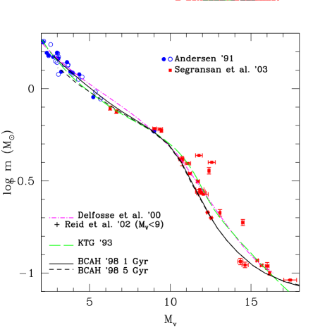
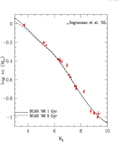
Figure 1: Comparison of the observed and theoretical m-$\mbox{M}_{V}$ relation.

Figure 2: Same for the m-$\mbox{M}_{K}$ relation.

3 The disk and young cluster mass function

3.1 The disk mass function

A V-band nearby LF $\Phi_{V}$ can be derived by combining Hipparcos parallax data (ESA 1997), which are essentially complete for $\mbox{M}_{V}<12$ at $r_{comp}$=10 pc, and the sample of nearby stars with ground-based parallaxes for $\mbox{M}_{V}>12$ with $r_{comp}$=5.2 pc ([Dahn86]). Such a sample has been reconsidered recently by [Reid02], and extended to r=8 pc by [Reid04]. The revised sample agrees within $\sim$1$\sigma$ with the previous one, except for $\mbox{M}_{V}\,\hbox{\hbox{$>$}\kern-8.00003pt\lower 4.30554pt\hbox{$\sim$}}\,14$, where the 2 LFs differ at the $\sim$2$\sigma$ limit. The 5-pc LF was also obtained in the H and K bands by [HMcC90].

The IMFs, $\xi(\log\,m)={dn\over d\log m}$, derived from the $\Phi_{V}$ and $\Phi_{K}$ LFs are portrayed in Figure 4 below 1 $\,\mbox{M}_{\odot}$. Superposed to the determinations is the following analytical parametrization (in $(\log\mbox{M}_{\odot})^{-1}\,\mbox{pc}^{-3}$):

$$\xi(\log\,m) = 0.093\times\exp\Bigl{\{}-{(\log\,m\,\,-\,\,\log\,0.2)^{2}\over 2\times(0.55)^{2}}\Bigr{\}},\,\,\,m\leq 1\,\,\mbox{M}_{\odot}$$ (1)

$$= 0.041\,m^{-1.35\pm 0.3}\,\,\,\,\,\,\,\,\,\,\,\,\,\,\,\,\,\,\,\,\,\,\,\,\,\,\,\,\,\,\,\,\,\,\,\,\,\,\,\,\,\,\,\,\,\,\,\,\,\,\,\,,m\geq 1\,\,\mbox{M}_{\odot}$$

This IMF differs a bit from the one derived in [Chabrier03a] since it is based on the revised 8-pc $\Phi_{V}$. The difference at the low-mass end between the two parametrizations reflects the present uncertainty at the faint end of the disk LF, near the H-burning limit (spectral types  $>$$\sim$  M5). Note that the field IMF is also representative of the bulge IMF (triangles), derived from the LF of [Zoccali00].

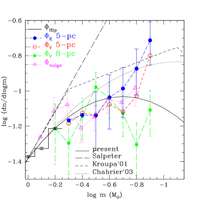
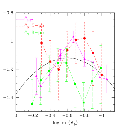
Figure 3: Disk IMF for individual objects.

Figure 4: Disk IMF for unresolved systems.

A fundamental advantage of the nearby LF is the identification of stellar companions. It is thus possible to merge the resolved objects into multiple systems, to calculate the magnitude of the systems and then derive the system IMF. The following parametrization, slightly different from the one derived in [Chabrier03a] is displayed in Figure 2 (normalyzed as eqn.(1) at 1 $\,\mbox{M}_{\odot}$, where all systems are resolved):

$$\xi(\log\,m)=0.076\times\exp\Bigl{\{}-{(\log\,m\,\,-\,\,\log\,0.25)^{2}\over 2\times 0.55^{2}}\Bigr{\}},\,\,\,m\leq 1\,\,\mbox{M}_{\odot}$$ (2)

As shown by [Chabrier03b] and seen on the figure, this system IMF is in excellent agreement with the MF derived from the revised HST phometric LF ([Zheng01], showing that the discrepancy between the MF derived from the nearby LF and the one derived from the HST stemmed primarily from unresolved companions in the HST field of view.

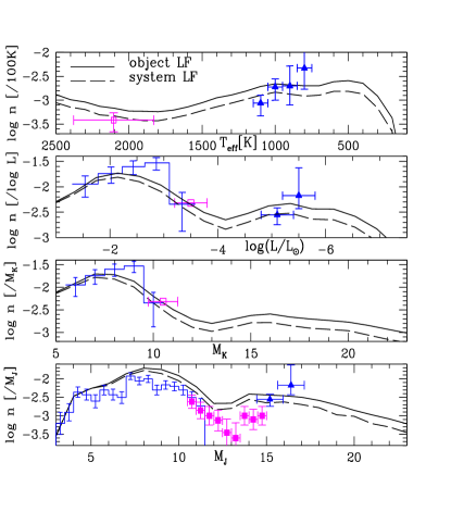
Figure 5: Comparison of the observed and theoretical LMS, L-dwarf ($\blacksquare$) and T-dwarf ($\blacktriangle$) distributions.

Figure 6: IMF for young clusters. Dash-line: field system IMF (2). Vertical dotted line: H-burning limit.

The brown dwarf regime.

Many brown dwarfs (BD) have now been identified down to a few jupiter masses in the Galactic field with the DENIS, 2MASS and SDSS surveys. Since by definition BDs never reach thermal equilibrium and keep fading with time, comparison of the predicted BD LFs, based on a given IMF, with observations requires to take into account time (i.e. formation rate) and mass (i.e. IMF) probability distributions. In the present review, we proceed slightly differently from the calculations of [Chabrier03a]. We start from the system IMF (2) and we include a probability distribution for the binary frequency which decreases with mass. Indeed, various surveys now show that the binary fraction $X_{bin}$ (and orbital separation) decreases with mass, varying from $X_{bin}\approx 60$% for G and K-stars to $\approx 40$% for early (M0-M4) M-dwarfs, to $\approx 20$% for later M and L-dwarfs, correcting for undetected short period binaries, to $\approx 10$% for T-dwarfs.

Figure 6 displays the calculated BD density distributions as a function of $T_{\rm eff}$, $L$, $\mbox{M}_{K}$ and $\mbox{M}_{J}$, based on the BD cooling models developed in the Lyon group, and the most recent estimated LMS and BD densities ([Gizis00, Burg01, Cruz04]